Discovering Gene Networks
Department of Computer Science
Faculty of Sciences at University of Porto
Discovering Gene Networks
Dissertation presented to Faculty of Sciences at University of Porto in partial fulfillment of the requirements for the degree of Master in Computer Science
Scientific Advisor: V´ıtor Manuel de Morais Santos Costa, PhD Scientific Co-Advisor: Irene May Lin Ong, PhD
Department of Computer Science Faculty of Sciences at University of Porto
a lot from him. I am grateful for his support, guidance and patience especially over this past year.
A special word of thanks to Irene Ong who also supported and helped a lot with the guidance of this work.
A very special thank and appreciation to my parents, who always helped, believed and encouraged me in every way they could so that I could have a proper education and also succeed in my professional life.
Also, a very special thanks and appreciation to my girlfriend Raquel, who never let me give up and always believed in me, and gave me her inconditional support every day.
Thanks also to Jeffrey Lewis who provided data and consulted.
A thanks to all my Masters teachers at DCC FCUP who inspired me to pursue knowledge discovery and research.
I also wish to thank the Fundac˜ao para a Ciˆencia e a Tecnologia. This work was supported with the FCT grant PTDC/EIA-EIA/100897/2008.
A word of appreciation to my friends and colleagues for the support.
Last, but not least, a thanks to my crazy cats Nero and Sasha who were always able to make me laugh when my work was not going very well at that time.
Transcriptional regulation plays an important role in every cellular decision. Gaining an understanding of the dynamics that govern how a cell will respond to diverse en-vironmental cues is difficult using intuition alone. In this work, logic-based regulation models based on state-of-the-art work on statistical relational learning are introduced, and evaluated on time-series gene expression data of the Hog1 pathway. Results show that plausible regulatory networks can be learned from time series gene expression data using a probabilistic logical model. Hence, network hypotheses can be generated from existing gene expression data for use by experimental biologists.
Keywords:-Gene Regulation, Network/Pathway Analysis, Statistical Re-lational Learning
Palavras-Chave: Regula¸c˜ao de Genes, An´alise de Redes/Caminhos, Apren-dizagem Relacional Estat´ıstica
Abstract 9 List of Tables 13 List of Figures 16 Acronyms 17 1 Introduction 19 1.1 Introduction . . . 21 1.2 Thesis Roadmap . . . 22 2 Biology Background 25 2.1 DNA . . . 27 2.2 RNA . . . 30 2.2.1 Structure . . . 31 2.2.2 Synthesis . . . 32 2.2.3 Types . . . 34
2.3 Gene Regulatory Networks . . . 36
2.4 Expression Data . . . 39
2.4.1 Data Measurement . . . 39
3.2 Logical models . . . 47
3.3 Other approaches . . . 50
4 Introduction to Logic Programming 53 4.1 Logic . . . 55
4.2 Binary Decision Diagrams . . . 58
4.2.1 Ordered Binary Decision Diagrams . . . 59
4.3 Problog . . . 63
4.3.1 Learning Problog Programs . . . 67
5 Implemented Work 69 5.1 Representing gene networks with Problog . . . 71
5.2 Experimental Methodology . . . 72 5.2.1 Implementation . . . 76 5.3 Results . . . 77 5.3.1 Problog Performance . . . 80 6 Conclusions 85 6.1 Conclusions . . . 87 6.2 Future Work . . . 87 A Code 89 References 98 12
4.1 Propositional logic symbols . . . 56
5.1 Variation in Correlation Between All Genes and Experiments Along Time 77
5.2 Analysis 2: proposed parents with threshold 0.7 ≤ P ≤ 0.9 . . . 78
5.3 Experiment 3 (VV): proposed parents per gate. Notice that + repre-sents the positive parent, and − the negative parent. . . 80
5.4 Experiment 3 (LV): proposed parents per gate. Notice that + repre-sents the positive parent, and − the negative parent. . . 80
5.5 Calculation times differences between the two ProbLog versions with no BDDs rebuild . . . 81
5.6 Calculation times differences between the two ProbLog versions with BDDs rebuild after 20 iterations . . . 82
5.7 Calculation times differences between the two ProbLog versions with BDDs rebuild after 45 iterations . . . 82
2.1 The flow on information in a cell, a.k.a. Central dogma of biology . . . 27
2.2 DNA Chemical Structure . . . 28
2.3 DNA double helix structure . . . 29
2.4 DNA base pairs . . . 29
2.5 DNA zipper . . . 30
2.6 RNA Chemical Structure . . . 31
2.7 RNA Secondary Structures . . . 32
2.8 Promoter Sequences . . . 33
2.9 RNA Synthesis . . . 33
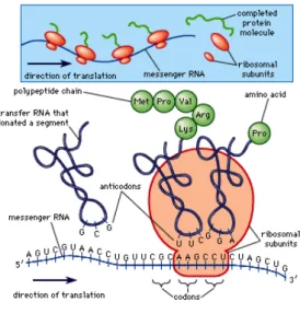
2.10 Messenger RNA . . . 34
2.11 RNA abundance in cells . . . 34
2.12 Transfer-messenger RNA . . . 35
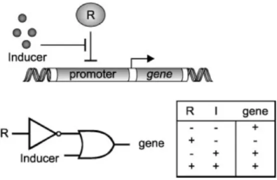
2.13 Example of an architecture of the inducible gene network . . . 36
2.14 Gene Regulation: The activation or inhibition of a gene transcription by one or several transcription factors. . . 38
2.15 Processes in a Gene Regulatory Network . . . 38
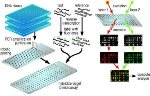
2.16 A general scheme for a microarray. . . 40
3.1 Example of a Boolean network . . . 47
4.2 Reduction of a BDD . . . 59
4.3 Both OBDDs are reduced, but they equivalent. Although only the left one is ordered [x, y, z]. . . 60
4.4 Execution of the reduce algorithm . . . 61
4.5 Two arguments for a call apply(+, Bf, Bg). . . 62
4.6 The recursive call structure for apply for example in Fig.4.5. . . 63
4.7 The result of apply(+, Bf, Bg). . . 63
4.8 A simple directed graph, where each edge has a probability of being true. 64 4.9 A BDD that computes the total probability of the path ae. . . 66
5.1 A simple BDD . . . 72
5.2 Implementation Method . . . 77
5.3 Same-step Correlation Generated Hog1 Promoter Network . . . 78
5.4 Learning Curves for Test Data Mean Square Error, resp for VV (∆ ⇒ ∆), VL (∆ ⇒ L) and LL (L ⇒ L). . . 79
5.5 Speedup graph based on Table 5.5 results . . . 81
5.6 Speedup graph based on Table 5.6 results . . . 82
5.7 Speedup graph based on Table 5.7 results . . . 83
AIK - Akaike’s Information Criterion
BDD - Binary Decision Diagram
BN - Bayesian Network
COD - Coefficient of Determination
CTL - Computation Tree Logic
CUDD - CU Decision Diagram
DBN - Dynamic Bayesian Network
DNA - Deoxyribonucleic acid
dsRNA - Double-stranded Ribonucleic acid
EM-algorithm - Expectation–Maximization algorithm
GE - Gene Expression
GRN - Gene Regulatory Network
GP - Genetic Programming
Lac - Lactose
LMS - Least Mean Square
LNA - Linear Noise Approximation
LTM - Linear Transcription Model
MAPK - Mitogen-activated protein kinases
Mg2+ - Magnesium
MWSLE - Minimum Weight Solutions to Linear Equations
Na+ - Sodium
NaCl - Sodium Chloride
ncRNA - Non-coding Ribonucleic acid
OBDD - Ordered Binary Decison Diagram
ODE - Ordinary Differential Equation
PBN - Probabilistic Boolean Network
PDE - Partial Differential Equation
PIN - Protein Interaction Network
PRM - Probabilistic Relational Model
PSN - Protein Signaling Network
RNA - Ribonucleic acid
RNAseq - Whole Transcriptome Shotgun Sequencing
rRNA - Ribosomal Ribonucleic acid
SDE - Stochastic Differential Equation
siRNA - Small interfering Ribonucleic acid
SRL - Statistical Relational Learning
SVD - Singular Value Decomposition
Tet - Tetracycline
tmRNA - Transfer-messenger Ribonucleic acid
tRNA - Transfer Ribonucleic acid
YAP - Yet Another Prolog
Introduction
If you don’t know where you are going, you’ll end up someplace else.
Yogi Berra
1.1
Introduction
Many major cellular decisions involve changes in transcriptional regulation. With the advent of high-throughput technologies and advanced measurement techniques molecular biologists and biochemists are rapidly identifying components of these net-works and determining their biochemical activities, but understanding these complex multicomponent networks that govern how a cell will respond to diverse environmental cues is difficult using intuition alone. In this work, our goal is to build a probabilistic logical model that can aid in uncovering the structure and dynamics of such networks and how they regulate their targets. Gaining insight into transcriptional regulation is important not just for understanding the fundamental biological processes, but also for advancing research.
A cell responds to environmental changes by detecting molecules that bind to receptors on the surface of the cell and transmits this information to proteins within the cell by activating a cascade of molecular events. These signaling networks are typically studied by measuring molecular events after treatments that stimulate or perturb key elements in the network at the mRNA or gene level. Combining these measurements with phenotypic response enables the study of these treatments on the architecture and function of the underlying signaling networks as well as the relationship between the network behavior and phenotypic response [1]. In this work, to infer the architecture and function of the underlying signaling network of budding yeast, we decided to focus on the pathways activated by MAPK1Hog1 during osmotic stress response. According
to previous results [2], this pathway interacts with the general stress (Msn2/Msn4) pathways, so we consider the genes belonging to both pathways in the following study.
Despite the challenge of inferring genetic regulatory networks from gene expression data, various computational models have been developed for regulatory network anal-ysis. Examples include approaches based on logical gates [3, 4], and probabilistic approaches, often based on bayesian networks [5]. On one hand, logic gates provide a natural, intuitive way to describe interactions between proteins and genes. On the other hand, probabilistic approaches can handle incomplete and imprecise data in a
1Mitogen-activated protein (MAP) kinases are serine/threonine-specific protein kinases belonging
to the CMGC (CDK/MAPK/GSK3/CLK) kinase group. These kinases regulate gene expression, proliferation, differentiation, mitosis, cell survival - among many others.
very robust way.
Our main contribution is in introducing a model that combines the two approaches. Our approach is based on the probabilistic logic programming language ProbLog [6, 7]. In this language, we can express true logical statements (expressed as true rules) about a world where there is uncertainty over data, expressed as probabilistic facts. In the setting of gene expression, this corresponds to establishing:
• a set of true rules describing what are the possible interactions existing in a cell; • a set of uncertain facts describing which possible rules are applicable to a certain
gene or set of genes.
Given time-series gene expression data, we want to choose the probability parameters that best describe the data. Our approach is to reduce this problem to an optimization problem, and use a gradient ascent algorithm to estimate a local solution [8] in the style of logistic regression. We further contribute an efficient implementation to this algorithm that computes both probabilities and gradients through binary decision diagrams (BDD).
We evaluate our approach by using it to study expression data on an important gene-expression pathway, the Hog1 pathway [2]. It is well known that under conditions of osmotic stress, the protein kinase Hog1, and the paralogous proteins Msn2 and Msn4 interact to create a response that involves the expression of a large number of proteins. We model these pathways by also incorporating the two transcription factors activated by Hog1: Hot1 and Sko1.
1.2
Thesis Roadmap
This thesis is divided into a total of six chapters. In Chapter 1 we present a small introduction to the biological process and the problem of discovering gene networks. In Chapter 2 we explain some important concepts for understanding the work in this thesis, we talk about DNA, RNA, gene regulatory networks and also about expression data, the data we use for our models. Next, in Chapter 3 we talk about related work in the area, presenting some of the techniques that can be used for creating gene regulatory networks. Chapter 4 is a brief introduction to logic programming and also concepts that are necessary for understanding the processes behind the calculations. A short introduction to Problog is also given. In Chapter 5 we explain how to represent
gene networks with Problog, how we perform our experiments and develop our models and we show the results we obtained. Last, Chapter 6 presents the conclusion we took from our work and we also talk about the future work we intend to perform.
Biology Background
Every biologist has at some time asked ’What is life?’ and none has ever given a satisfactory answer. Science is built on the premise that Nature answers intelligent questions intelligently; so if no answer exists, there must be something wrong with the question.
Albert Szent-Gy¨orgyi
In this chapter we will explain some fundamental biological concepts that will be important for understanding this work. We will start by discussing DNA, one of the fundamental basis of life, then we will survey RNA, which is usually created by DNA (although there are some exceptions in retro-viruses such as Human Immunod-eficiency Virus (HIV)). Afterwards an introduction to gene regulatory networks will be presented and finally we will present the data used for this type of work, where it comes from, how it is obtained and what it provides.
One of the goals in computational biology is to understand the regulation processes in a cell at the gene level, which can in turn lead to specific interventions for genetic diseases and drug design [9]. The global understanding of an organism in great detail is a long term goal, as is the understanding and analysis of the information flow in a cell (Fig. 2.1)
Figure 2.1: The flow on information in a cell, a.k.a. Central dogma of biology
2.1
DNA
The deoxyribonucleic acid (DNA) is a nucleic acid containing the genetic instructions used in the development and functioning of all known living organisms (with the exception of RNA viruses). DNA contains segments known as genes that carry the genetic information. This acid is one of the three major macromolecules that are essential for all known forms of life, the other two macromolecules are RNA and
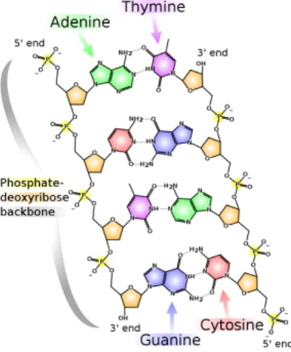
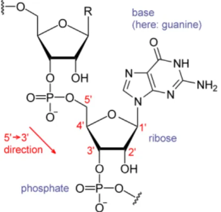
proteins. DNA is composed of two nucleotides (molecules that make up the individual structural units), with backbones made of sugars and also phosphate groups [10] that are joined by ester (chemical compound consisting of a carbonyl adjacent to an ether linkage) bonds. The sugars are joined together by phosphate groups that form phosphodiester bonds (Fig. 2.2) between the third and fifth carbon atoms of adjacent sugar rings. These bonds are asymmetric, hence a strand of DNA has a direction. Notice that the two strands are anti-parallel, that is, they run in opposite directions to each other. Attached to each sugar is one of the four nucleobases of DNA: Adenine (A), Cytosine (C), Guanine (G), Thymine (T). These nucleobases are
Figure 2.2: DNA Chemical Structure
classified into two types: the purines, A and G, are fused five- and six-membered heterocyclic compounds, and the pyrimidines, are six-membered rings C and T [11]. Information is encoded by this sequence of bases along the backbone, and one can say that DNA is a long polymer made from repeating units called nucleotides[12], [13]. In order to read this information, the genetic code that specifies the sequence of amino acids within proteins is used. The reading of the code is done through a process called transcription (the process of creating a complementary RNA copy of a sequence of DNA), we will describe it further in the next section. DNA is organized within cells by using chromosomes, which are duplicated in the process of DNA replication. Due to this replication, each cell has its own complete set of chromosomes. On the other hand, DNA is organized and compacted within the chromosomes by chromatin proteins, creating a type of compact structures that are responsible for guiding the interactions between DNA and other proteins and which help control which parts of DNA are transcribed.
entwined vines, forming the known shape of a double helix [14] as shown in Fig. 2.3. The nucleotide repeats contain both the segment of the backbone of the molecule, which holds the chain together, and a nucleobase, which interacts with the other DNA strand in the helix[15]. As we discussed earlier, DNA has two asymmetric ends which are known as the 5’ (five prime) and 3’ (three prime) ends. The five prime has a terminal phosphate group and the three prime has a terminal hydroxil group as shown in Fig. 2.2. In a DNA double helix there is a property called complementary
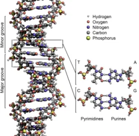
Figure 2.3: DNA double helix structure
base pairing, which is defined by the fact that each type of nucleobase on one strand normally interacts with just one type of nucleobase on the other strand, A only bonds to T and C only bonds to G forming the base pairs shown in Fig.2.4. The two base
Figure 2.4: DNA base pairs
and GC forms three hydrogen bonds, therefore, DNA with high GC -content is said to be more stable than DNA with low GC -content. Due to the non-covalent property of hydrogen bonds, these can be broken and rejoined easily. This enables the strands of DNA to be pulled apart like a zipper, using high temperature or even a mechanical force [16]. Notice that, all the information in the double-stranded sequence of a DNA
Figure 2.5: DNA zipper
helix is duplicated on each of the strands, which is vital in DNA replication (the basis for biological inheritance). This reversible interaction between complementary base pairs is critical for all the functions of DNA in living organisms.
2.2
RNA
The Ribonucleic acid (RNA) is a biologically important type of molecule that consists of a long chain of nucleotide units, it is one of the four major macromolecules (along with lipids, carbohydrates and proteins) and essential for all known forms of life, but it differs from DNA: RNA is usually single-stranded in the cell, while DNA is usually double-stranded; RNA nucleotides contain ribose while DNA contains deoxyribose (a type of ribose that lacks one oxygen atom), as there is no hydroxyl group attached to the pentose ring in the 2’ position in DNA; and RNA has the base uracil rather than thymine that is present in DNA. The sequence of nucleotides allows RNA to encode genetic information. RNA is transcribed from DNA by enzymes called RNA polymerases and is generally further processed by other enzymes. RNA is in the center of protein synthesis, as a type of RNA called messenger RNA (mRNA) carries information from DNA to cellular structures called ribosomes. It is also known that many viruses use RNA instead of DNA as their genetic material.
Ribosomes are made from ribosomal RNAs (rRNAs) and proteins, which come to-gether to form a type of molecular machine that is able to read the mRNAs and translate their information into proteins. This is attained by a process that uses transfer RNA (tRNA) molecules to deliver amino acids to the ribosome, where ribo-somal RNA (rRNA) links amino acids together to form the proteins. Other types of RNA molecules play an active role in cells by controlling gene expression, sensing and
communicating responses to cellular signals or catalyzing biological reactions. Most RNA molecules are single-stranded and can adopt very complex three-dimensional structures as described next.
2.2.1
Structure
Each one of RNA’s nucleotides contain a ribose sugar, this sugar has carbons num-bered from 1’ through 5’. A base, usually Cytosine (C), Adenine (A), Uracil (U), Guanine(G), is attached to the 1’ position. Cytosine and uracil are pyrimidines, guanine and adenine are purines. Attached to the 3’ position of one ribose and to the 5’ position of the next is a phosphate group, these groups have a negative charge at physiological pH, which makes RNA a charged a molecule (polyanion). It is known that the bases may form hydrogen bonds between guanine and uracil, between cytosine and guanine and also between adenine and uracil. Besides these bases, there are numerous modified bases and sugars in mature RNAs, some example are the Pseudouridine -in this base the l-inkage between uracil and ribose is changed from a C-N bond to a CC bond (usually found in the TC loop of tRNA [17]) and the Hypoxanthine -a de-amin-ated -adenine b-ase whose nucleoside is c-alled inosine (I), which pl-ays -a key role in the wobble hypothesis (a non-Watson-Crick base pairing composed by two nucleotides in RNA molecules) of the genetic code. One of the important structural
Figure 2.6: RNA Chemical Structure
features that distinguishes RNA from DNA is the presence of a hydroxil group at the 2’ position of the ribosome sugar, which causes the helix to adopt an A-form geometry instead of the B-form that is commonly observed in DNA [18]. The presence of the 2’-hydroxil group also has another consequence, in conformationally flexible regions of a RNA molecule (not involved in formation of a double helix) it can chemically attack
the adjacent phosphodiester bond to split the backbone [19].
It is known to exist about 100 naturally occurring modified nucleosides, although the specific role of these modifications in RNA are not yet fully understood. Many of the post-transcriptional modifications occur in highly functional regions, which implies that they are important for normal function. Frequently, the functional form of single stranded RNA molecules require a specific tertiary structure which is provided by the secondary structural elements (hydrogen bonds within the molecule). The result of this are the recognizable secondary structure known as hairpin loops, bulges and also internal loops, as shown in Fig. 2.7.
Figure 2.7: RNA Secondary Structures
RNA is charged, so in order to stabilize many secondary and tertiary structures, metal ions such as M g2+ and N a+ are needed as loop information is unfavorable
due to backbone charge-charge repulsion. These two metal ions can increase the loop flexibility by neutralizing the phosphate charges, causing the loop formation to be less unfavorable. The result of increasing M g2+ and N a+ is a decrease on the energy cost
for loop formation [20].
2.2.2
Synthesis
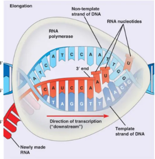
RNA synthesis, or transcription is under the control of the enzyme RNA polymerase. The first step that this enzyme takes is to find the start of the gene on the coding
strand of the DNA, as the DNA has lots of genes strung out along the coding strand (the enzyme has to pick the right strand and identify the beginning of each gene). This is done by recognizing and binding with one or more short sequences of bases (also known as promoter sequences, Fig. 2.8) ”upstream” of the start of each gene. The transcription process (Fig. 2.9) is composed of the following steps:
Figure 2.8: Promoter Sequences
• The DNA double helix is unwound due to the helicase activity of the enzyme • Enzyme progression along the template strand following the 3’ to 5’ direction • Synthesis of a complementary RNA molecule
Figure 2.9: RNA Synthesis
The end of RNA synthesis is indicated by the DNA sequence. RNAs are often modified by enzymes after transcription. There are also a number of RNA-dependent RNA polymerases that use RNA as their template for synthesis of a new strand of RNA. For instance, a number of RNA viruses use this type of enzyme to replicate their genetic material.
2.2.3
Types
There are several types of RNA, as discussed before:
• Messenger RNA (mRNA) - molecule in cells that carry codes from the DNA to the sites of protein synthesis (the ribosomes). Information in DNA cannot be decoded directly into proteins, and thus it is first transcribed, or copied, into mRNA. Each molecule of mRNA encodes the information for one protein (or more than one protein in the case of a bacteria), with each sequence of three nitrogen-containing bases in the mRNA. The mRNA takes the copy of the blueprint to the ribosome where it is used to build the protein.
Figure 2.10: Messenger RNA
• Ribosomal RNA (rRNA) - these molecules form the structural and functional components of ribosomes, the subcellular units responsible for protein synthesis [21]. This type of RNA is the catalytic component of the ribosomes. rRNA
constitutes approximately 80% to 85% of the total RNA in a cell (shown in Fig. 2.11). In eukaryotes, rRNA synthesis occurs in the nucleolus, a specialized structure within the nucleus.
• Transfer-messenger RNA (tmRNA) - molecule of RNA (found in many bacteria and plastids) that has dual functions as both a transfer RNA and a messenger RNA. As a tRNA, it recognizes and binds ribosomes stalled by aberrant mRNAs with the help of its protein partner SmpB. As an mRNA, it adds a degradation tag to protein fragments, targeting them for proteolysis. Two types of tmRNAs are known: single-chain tmRNAs and two-piece tmRNAs.
Figure 2.12: Transfer-messenger RNA
• Non-coding RNA (ncRNA) - functional molecule that is not translated into protein. ncRNAs have been shown to regulate important biological processes that support normal cellular functions, but relatively little is known about the general structure, function, and transcriptional control of ncRNAs, and even less about their potential functions as a group or as a single entity [22].
• Other types of RNA are the following: Doublestranded RNA (dsRNA) -RNA with two complementary strands, similar to the DNA found in all cells. dsRNA forms the genetic material of some viruses (dsRNA viruses). dsRNA such as viral RNA or siRNA can trigger RNA interference in eukaryotes, as well as interferon response in vertebrates. MicroRNA (miRNA) - small type of dsRNA molecules that regulate translation in eukariotic cells, it is related to RNAi. Unlike other small RNAs, the genes for miRNA are transcribed by RNA polymerase II. MicroRNAs are not only used in eukariotic cells but also by some of the more complex viruses that infect them. Short-interfering RNA (siRNA) - short dsRNA fragments that are known to bound by the the RNA-induced silencing complex1 (RISC) [23]. It is class of double-stranded RNA molecules
1RNA-induced silencing complex, or RISC, is a multiprotein complex that incorporates one strand
that play many roles, being the most notable the RNA interference (RNAi) pathway.
2.3
Gene Regulatory Networks
Every cell is a complex processor of information, as it is able to integrate and respond to multiple signals in a robust way. The mechanism that cells use to achieve this are remarkable and in a large number. One can make an analogy to electrical circuits, that is, we can decompose the high complexity involved in cellular response into modules that connect to each other by input and output signals [24]. We can take this comparison a little further, as genetic network engineers manipulate living organisms using the biological equivalent of transistors and inverters. A possible description of gene networks is circuits of interconnected functional modules, each consisting of specialized interactions (information flow) between proteins, RNA, DNA and small molecules. The importance of these modules (components) can be exemplified by their
Figure 2.13: Example of an architecture of the inducible gene network
use in networks that function in cells that have a higher complexity. An advantage of prokaryotic components such as repressors and their operating sites is that they can be transplanted into eukaryotic cells without any loss of their binding or function specificity. A second advantage is the avoidance of unwanted interference with the expression of non-targeted genes [24]. There has been a large development of switch systems based on the Tet or Lac repressor in a large number of organisms ([25], [26], [27], [28]). This development sets the stage for the construction of more complex gene networks.
template for recognizing complementary mRNA. When it finds a complementary strand, it activates RNase and cleaves the RNA.
In order to synthesize proteins that carry out specific functions in the cell, this information is extracted through a process called gene expression. On the other hand, gene regulation describes all the cellular processes which control the expression of proteins. This regulation can occur at the following steps of the DNA information extraction:
• Transcription initiation - start of the binding of RNA polymerase to the promoter in DNA
• Translation - the mRNA produced by transcription is decoded by the ribosome in order to produce a polypeptide, or a specific amino acid chain, that will later fold into an active protein.
• Modifications of mRNAs - modified to remove certain stretches of non-coding sequences called introns.
• DNA packing - process in which DNA and associated proteins are formed into a compact, orderly structure.
• Post-translational modifications of amino-acid sequences - this modification ex-tends the range of functions of the protein by attaching it to other biochemical functional groups, making structural changes, or changing the chemical nature of an amino-acid.
There are many different gene expression patterns in a cell, they depend of factors like the state of the cell, nutrition, environment or even the cell type. The process of gene expression consists of translation and transcription, with the regulation of this expression taking place at different steps, but usually more during transcription (truest when talking about procaryotes like bacteria). As exons and introns are not distinguished in their mRNA molecules, an alternative splicing (one of the more relevant regulation processes taking place after the transcription step [29])takes place, leading to different proteins from the same mRNA molecule. In order to build a model for gene regulation, one needs to specify the interactions (the ones that the dynamic behavior of gene expression can be explained by them) that should be captured by the model.
The transcription of a gene can be activated or inhibited by transcription factors which can bind to a site on the DNA near the promoter (the place where the following gene transcription is started) in a way that the transcription factor that binds inhibits the
Figure 2.14: Gene Regulation: The activation or inhibition of a gene transcription by one or several transcription factors.
start of the transcription. In order to activate a transcription, transcription factors can absorb other molecules that bind to that particular site. We can see different possibilities of inhibition and activation in Fig. 2.14. The product of a gene can regulate its own transcription or of another gene, it can also regulate the expression with the help of other products of genes.
Regulatory proteins and their binding sites are also modular in that different domains from different proteins can be combined to yield hybrid proteins of novel function. The state in which a living organism is at any certain point of time is not only described by its genome, but also by its set of expressed regulatory genes and its concentration levels of the corresponding gene products. All the possible phenotypic states of a cell correspond to distinct gene expression patterns [30].
Figure 2.15: Processes in a Gene Regulatory Network
To sum all up, we can say that gene regulatory networks (GRNs) are interacting DNA-encoded regulatory subsystems in the Genome that have the function of coor-dinating the inputs from activators and repressors (Transcription Factors) during cell differentiation, development or even in response to environmental causes (natural or
not). GRNs funtion to specify expression of particular sets of genes for specific times, locations and conditions.
2.4
Expression Data
In order to sequence the human genome, methods for measuring the expression levels of single and all genes simultaneously in a genome had to be created. An existing challenge of Computational Biology is the analysis of thousands of measurements of one cell state in order to retrieve the useful information from it. To get these measures, Microarray Technology 2 is applied. By using this technology, the researchers can
observe the dependency of gene expression on different states of a cell and also on different environmental factors.
2.4.1
Data Measurement
The description of any model gets better as more relevant information becomes avail-able. This seems trivial as huge amounts of information exist nowadays, but unfor-tunately for gene regulation that is not true, some of the data available is only for selected targets, which some of the times are not satisfactorily accessible and most of the data is very noisy. The advance in DNA-microarray technology permits to monitor thousands of genes in one experiment by measuring mRNA concentrations in a cell [31]. Each data point produced by a DNA microarray experiment represents the ratio of expression levels of a particular gene. The result, from an experiment with n genes on a single chip, is a series of n expression-level ratios. Typically, the numerator of each ratio is the expression level of the gene in the varying condition of interest, whereas the denominator is the expression level of the gene in some reference condition. The data from a series of m such experiments may be represented as a gene expression matrix, in which each of the n rows consists of an m-element expression vector for a single gene. The expression measurement is positive if the gene is induced (turned up) with respect to the reference state and negative if it is repressed (turned down). Every spot on the microarray has millions of copies of one probe in order
2An array is an orderly arrangement of samples where matching of known and unknown DNA
samples is done based on base pairing rules. An array experiment makes use of common assay systems such as microplates or standard blotting membranes. The sample spot sizes are typically less than 200 microns in diameter usually contain thousands of spots
Figure 2.16: A general scheme for a microarray.
to measure not only the existence of specific mRNA in the test material, but also to measure its amount, making it interesting if time series are produced, such that the difference between two time points can give a hint for genes that are transcribed together or even a hint for some regulatory interactions.
Related Work
Knowing is not enough; we must apply.
Willing is not enough; we must do. Johann Wolfgang von Goethe
Throughout time there has been a lot of research regarding gene regulatory networks, their interaction, modeling and prediction. A number of mathematical models have been created in order to capture the behavior of the system that is being modeled, and also to generate predictions that are then validated through experimental observation. In some cases, the created models made some accurate novel predictions that were validated afterwards, leading advances in the biological field. Sometimes, these new discoveries could have not been found if it was not for the mathematical model, as the scientists would have not considered doing the experiment in a laboratory environment.
The most common techniques applied to the models are differential equations, Boolean networks, Bayesian networks and graphical models. Logic-based modeling is seen as an approach lying midway between the complexity and precision of differential equations on one hand and data-driven regression approaches on the other [1]. In the next subsections we will have a look at some related work using those techniques.
Clustering algorithms have also been used since the first works in gene expression, they have been primarily used to group together genes with similar temporal expression patterns [32], some work using this type of algorithms are [33] [34] [35] [36] [37]. The motivation for using this type of algorithms is the idea that two genes that exhibit a similar expression pattern over time may be coregulated by a third gene or even regulate each other.
3.1
Differential equations models
Within the spectrum of modeling methods currently being applied to cellular bio-chemistry, models involving differential equations bear the closest relationship to the underlying biochemical rate laws, and thus they are one of the most important modeling formalisms in mathematical biology.
Sets of coupled ordinary differential equations (ODEs) can effectively represent chem-ical reactions when the number of molecules is large and mass action approximations are appropriate. Partial differential equations (PDEs) add the ability to represent spatial gradients, and stochastic methods make it possible to analyze systems in which the number of molecules is small. Networks of differential equations can model the temporal and spatial dynamics of biochemical processes in considerable detail, making it possible to study chemical mechanisms and to predict network dynamics
under various conditions. What makes this type of equations adequate for gene expression is that they can also model complex dynamic behavior like oscillations, cyclic patterns, multi-stationary and switch-like behavior [9]. However, the topology (how species interact, their patterns of interaction) of ODE- and PDE-based models must be specified in advance, and model output is strongly dependent on the values of free parameters (usually the initial protein concentrations and rate constants). This parameters estimation is a computationally intensive task requiring substantial data. As networks get larger, ODE modeling becomes more and more challenging, and models that attempt to capture real biological data are currently limited to a few dozen components.
When using these equations, the first step is to find the ones that are more adequate to the problem at hand. In order to do so, we need large amounts of data (to infer the unknown parameters) and also the processes in the system that we are studying. Knowing which gene regulates which one, the way of the regulation, the degradation and the maximal production rates of the associated proteins is also very valuable knowledge.
Describing a gene network in terms of differential equations has 2 advantages [38]:
• It describes gene interactions in an explicitly numerical form
• Due to the large amount of information in a system of differential equations, other networks can be derived from it
There has been some development using differential equations to create models for gene regulation. Chen et al. [39] built a Linear Transcription Model based on linear differential equations and two algorithms to solve the differential equations. For their model they consider nRNA as well as protein data and use an equation like y = M y, where y(t) contains the protein and mRNA concentrations at time point t and M is a constant matrix, describing the influence that the variables have on each others change of concentration. Their approach had limitations, the model does not consider time delays in transcription or translation leading to a very significant reduction of the problem complexity. Another significant limitation comes from ignorance of other regulators. Despite these limitations, the LT model is able to clearly capture more features of gene expression than other models. An approach with MWSLE (Minimum Weight Solutions to Linear Equations) was also used, but the actual number of gene regulators was much larger than expected and the solution would probably be computationally intractable.
Following Chen et al. [39] work, De Hoon et al. [40] built a model focusing only on mRNA values. In their work they proposed to infer the degree of sparseness of the gene regulatory network from the data they had by determining which coefficients are nonzero by using Akaike’s Information Criterion for the task. The algorithm created by them estimates matrix M on the basis of maximum likelihood estimation and then uses AIK to estimate both position and number of nonzero parameters that the matrix contains. Their method allows for loops to be present in the network, these loops are only found if the measured data warrant them, the existence of them is not dictated. With this method they were able to present some interesting results on the transcription of Bacillus Subtilis [38]. The drawback of both models is that the matrix is assumed to be constant, leading to a failure to capture a lot of phenomenon in the dynamic behavior of a real organism.
Sakamoto et al. [41] developed a model that describes the expression change for the i -th gene as Xi = fi(x1, · · · , xn) (i = 1, 2, · · · , n) with possible nonlinear functions fi,
where Xi is the state variable and n is the number of components in the network. In
order to identify the system of differential equations, they use Genetic Programming (GP) to evolve the right hand side of the equation from the observed time series of the gene’s expression. They apply and combine two different methods of optimization, GP and Least Mean Square (LMS), the reason to do so is that GP is capable of finding a desirable structure effectively, but when one needs to optimize the constants or coefficients, ordinary GP is not always effective as it relies mainly on the combination of randomly generated constants. By using LMS one can explore the search space more effectively. Through using these methods Sakamoto et al. were able to successfully infer their network by several experiments, and were able to capture more behaviors than a linear model. One has to bear in mind that there may exist more than one solution for the target, that is, like many other models, a solution which fits the time series in a good way is not necessary the unique.
Gebert et al. [9] also built a model with differential equations in which they captured the most relevant regulating interactions and calculated the parameters for the model from time-series data. In order to do so they used piecewise linear differential equa-tions, that are originated from a decomposition of the state space into cuboids. They base their model on the assumption that regulation between genes can be described using piecewise linear functions. On their model, every single cuboid, differential equation is turned into a ordinary linear equation that can be solved analytically. They did have a need to solve the problem of estimating the parameters for each linear equation, leading it to an optimization problem which was resolved resticting
the solution space, that is, they included biological knowledge about the regulatory network. Although their model gets good results it is not yet ready for all organisms, as it requires a lot of input data to determine all unknown parameters (still not available).
Also in the field of differential equations we have the work of Fearnhead et al. [30] in which they use Linear Noise Approximation (LNA) as a compromise between the ODE and stochastic differential equations (SDE) models. Usually inference is performed by approximating the dynamics through an ODE or a SDE, but we are presented with two known problems: ODEs ignore the stochasticity in the true model and this can lead to inaccurate inferences, on the other hand, SDEs are more accurate than the former but they are harder to implement due to the transition density if the SDE models being generally unknown. In their work they use LNA as an approximation for inference due to the fact that models based on ODEs are usually appropriate for very large systems in which the stochasticity in the evolution is small, and also because SDE models are more appropriate for medium-size systems and these lead to sensible estimates of the reaction rates [30]. Due to these reasons and also knowing that the inference for SDE models is not trivial they use an alternative aproximation which first appeared on [42] and [43]. The LNA is obtained from two steps, first we must approximate the dynamics by a system of ODEs and second we must model the evolution of the state about the ODE deterministic solution using for this task a linear SDE. Although simulation suggests that the LNA approach has similar accuracy to the SDE, one must bear in mind that by using LNA the stochastic model for the states is a Gaussian process, which means that the mean and covariance of the transition densities can be found using a system of differential equations. Results presented by Fearnhead et al. [30] suggest that the usage of LNA gives more accuracy than approximating the underlying model using an ODE.
Akutsu et al. [44] present a model that can be considered as an intermediate model between differential equations and boolean networks (the algorithms are based on linear differential equations). In their model, regulation rules are embedded in network structures and are represented as quantitative rules. One of the algorithms presented by them can be applied to S-systems [45] [46] [47], these systems are based on a particular kind of nonlinear differential equations. Although their methods seem interesting they have some drawbacks, first it requires a lot of time series data from different sets of initial values (diferent conditions or even environments), this may not always be available, the second drawback is that complex enzymatic reactions can not be handled directly. In order to infer correctly they would have to focus only on a part of the network, as this would require less time series data.
In some other studies presented by di Bernardo et al. [48], Gardner et al. [49] and Bansal et al. [50] there has been a development of ODE-based algorithms that use a series of steady-state RNA expression measurements or even time-series measurements. There are also some other cases based on ODEs that can be found in the literature, some of them are the work by van Someren et al. [51], Tegner et al. [52], Bonneau et al. [53], D’haeseleer et al. [54] and de Jong et al. [32].
3.2
Logical models
Most often GRNs (Gene Regulatory Networks) are represented by using logical models. In these models, the gene-expression measurements are converted to discrete levels (on/off ), but this process usually introduces inconsistencies into the data. Is is believed that the reconstruction of a logical GRN that is able to minimize the errors is NP-complete, which suggests that an efficient algorithm to solve this problem may not exist. Even with these problems that have been several approaches that propose applying logical models. In deed boolean networks are used on many of the models present in the literature, we can have the state of a gene converted to a boolean variable that is in one of two possible states, active (1, on) or inactive (0, off ), meaning that the gene products are present or not. The interactions between elements of the network can be represented by boolean functions that are used to calculate the resulting state of a gene due to the activation of other genes. All of this culminates in the creation of a boolean network, as we can see in Fig. 3.1. An approach that includes boolean
Figure 3.1: Example of a Boolean network
networks is the approach by Akutsu et al. [55], in their work they define a GRN through the boolean network G = (V, F ) where V is the set of nodes and the set {F = fv|v ∈ V } of boolean functions assigned to the nodes, where the network may
have cycles. They also define a global state of G as being a mapping ψ : V → {0, 1} in which each global state must satisfy ψ(xi) = 1 and ψ(yi) = 0 under an experiment
hx1, . . . , xp, ¬y1, . . . , ¬yqi. In order to identify a GRN from observed global states they
investigate the number of experiments together with the cost of each experiment. This work lead to two important problems obtained from the identification of GRNs:
• consistency (checking if a network G0 = (V0, F0) coincides or not with the
underlying GRN)
• stability (G is stable if there exists a global state consistent with all gene regu-lation rules) of the network
Also, in their work they have derived upper and lower bounds on the required pertur-bations for the boolean networks.
Another approach using boolean networks is the work developed by Ideker et al. [56]) in which they present two methods (Predictor and Chooser ) for inferring a genetic network given gene expression measurements. The Predictor method is used to infer hypothetical boolean networks consistent with a profile that was generated previously by exposing the network of interest to a series of genetic or biological perturbations. After the inference of several networks, the Predictor method returns the ones that are most parsimonious (the ones having the fewest number of interactions). The next step is done by the Chooser method that adds an additional perturbation experiment in order to discriminate along the set of previously obtained hypothetical networks. These perturbations are added in a clever way by using a function that is based on en-tropy to optimally reduce the number of remaining hypothetical networks. One other feature of these two methods is that they can be used interactively and iteratively. Standard boolean networks have a very salient limitation, their inherent determinism. One can look at this from two points of view, the conceptual point of view or the empirical point of view. From the former, one must bear in mind that is likely that the regularity of genetic function and interaction known to exist is not due to hard-wired logical rules, as for the latter, it takes in account that one logical rule per gene may to incorrect results when these rules are being inferred from gene expression measurements. To address these considerations Shmulevich et al. [57] introduced a new model class, the Probabilistic Boolean Networks (PBNs), which have the properties of boolean networks and can cope with uncertainty in the data and model selection. The basic idea of their work is to extend the boolean network in order to accommodate more than one possible function for each node. For this, they have a set Fi = {f
(i)
j }j = 1, . . . , l(i) that corresponds to each node xi and where
number of possible functions for gene xi. For inferring they use a method based on the
Coefficient of Determination (COD) which produce a number of candidate predictors for each target gene. In this model, the approach was to probabilistically ’create’ good predictors so that each predictor contribution is proportional to its determinative potential, this is close to our own approach.
Also in this field of logical models, but on a more formal approach, we have the work by Bernot et al. [58] where they provide a formal way to treat temporal properties of biological regulatory networks, expressed in computational tree logic leading to the possibility of building all the models that satisfy a set of given temporal properties. Their work allows biology to take advantage from all the available formal methods from computer science, temporal properties can be checked against models using Computation Tree Logic (CTL) and model checking.
Still in the formal approach, we have the work by Batt et al. [59] that validates models of GRNs by addressing the challenge matching model predictions and experimental data, taking also in account a reliable and efficient comparison between the obser-vations and the predictions. The qualitative modeling and simulation method that they use is based in a refinement of previous work [60]. What is new about their work is that they use model-checking techniques to attend the problem that the state transition graphs that are generated by qualitative simulation may become very large in a way that it may be prohibitive for interesting biological networks.
An interesting work involving logical analysis it the one presented by Thomas et al. [61] where they present a logical method for the analysis of the complex dynamics of regulatory networks in terms of feedback circuits. The feature that distinguishes the most their work from others is that the logical method introduced by them is fully asynchronous, that is, current variables are discrete, but time is continuous. Besides this work presented by Thomas et al., they also have published other interesting ones related to logical models, their analysis and creation [62] [63] [64][65].
In recent work by Handorf et al., we are presented with a new method for an automated generation of boolean network models from curated mechanistic network databases. This straight forward method translates into a good gain that is even more important in the context of the fast growing amount of interactions available in these databases. Despite of this great advantage, there is also a drawback that is common to all boolean approaches, interactions strengths and concentrations can not be properly covered by TRUE and FALSE values.
Further work has been developed in the area of GRNs using logic models [66] [67] [68] and even logic tools to model and analyze signaling pathways [69].
3.3
Other approaches
At the other extreme, a very active field in computing graphical representations of biological networks [70] [71] through literature analysis or through identification of correlations in high-throughput data has emerged. In these graphs, termed protein interaction networks (PINs or interactomes) or protein signaling networks (PSNs), genes and proteins are represented by nodes and potential interactions by edges (links). The edges can be directional or not and signed (inhibitory/activating) or not and typically represent a wide range of interaction modes from direct physical binding to correlated gene expression or integrated database entries. Graphs are an attractive way to summarize diverse relationships among large numbers of biomolecules across multiple organisms, but they are not executable per se and cannot be used to com-pute input-output relationships. Moreover, network graphs rarely take into account dynamic changes in signaling activities, cell type-specific biochemistry, or context-dependent variations.
Despite the difficulty of deciphering genetic regulatory networks from microarray data, numerous approaches to the task have been quite successful. Friedman et al. [5] were the first to address the task of determining properties of the transcriptional program of S. cerevisiae (yeast) by using Bayesian networks (BNs) to analyze gene expression data. Pe’er et al. [72] followed up that work by using BNs to learn master regulator sets. Other graphical approaches are Tanay and Shamir [73], Chrisman et al. [74]). The former implemented a new software platform called Genesis to enable analysis of available transcription profile data sets and target pathways. The latter present a Bayesian framework which combines information from several different sources and makes the correct causal inferences with small sample sizes.
The methods above can represent the dependence between interacting genes, but they cannot capture causal relationships. Pe’er et al. [72] ingeniously proposed the use of microarray experiments in which specific genes have been deleted (knockout) in yeast to obtain causality. The use of perturbations such as gene deletion mutants can allow the BN learning algorithm to learn a directed edge that suggests direct causal influence. This approach of combining observational and interventional data delivered promising results. Unfortunately, a complete library of gene knockouts are
not yet available for organisms other than yeast. The advent of small interfering RNA (siRNA) can be used to reduce the expression of a specific gene in organisms other than yeast, however, siRNA does not guarantee complete silencing of the gene. Ong et al. [75], proposed that the analysis of time series gene expression microarray data using Dynamic Bayesian networks (DBNs) could allow to learn potential causal relationships. DBNs are usually based on discrete models [76] [77] [78] or on continuous time models [79].
Another approach, is the work by Perrin et al.[80]. In their work they used penalized likelihood maximization in EM-algorithms to learn the parameters for a DBN. Dojer et al. [81] also apply DBNs, but this time in the context of perturbation experiments. With the incorporation of this type of data they are able to check that the quality of inferred networks dramatically improves.
A different approach is presented by Yeung et al. [82] who propose a scheme to reverse-engineer gene networks using Singular Value Decomposition (SVD) to construct a set of candidate solutions and afterwards applies robust regression to identify the solution with the smallest number of connections.
Last, we refer the reader to Madeira et.al [83], a work where biclustering algorithms for biological data analysis are described and analyzed. Biclustering algorithms have been used for some time now, the first time the term was used in gene expression data analysis was by Cheng et. al [84]. The main difference between these type of algorithms and the simple clustering algorithms is that the second ones can be applied to columns or rows of the data matrix (each at a time), but the first algorithms can perform clustering on the two dimensions (rows and columns) at the same time -meaning that with biclustering produces a local model while clustering produces a global model. With this we can say that the goal of biclustering algorithms is to identify genes subgroups and conditions subgroups by performing clustering on the rows and columns of the gene expression data matrix at the same time. Contrary to the clustering algorithms, biclustering is able to find sets of genes that have similar activity under a specific set of conditions.
Introduction to Logic Programming
Logic is not a body of doctrine, but a mirror-image of the world. Logic is transcendental.
Ludwig Wittgenstein
In this chapter we will talk about Propositional logic (also known as sentential logic, is that branch of logic that studies ways of combining or altering statements or propo-sitions to form more complicated statements or propopropo-sitions) as a small introduction prior to talking about Binary Decision Diagrams (data structures for representing the semantics of a formula in propositional logic) and Ordered Binary Decisions Diagrams of which we show three algorithms that can be performed on them (Reduce, Apply, Restrict ). Next we talk about Problog, giving the fundamental ideas of how it works and how it is implemented.
4.1
Logic
The objective of propositional logic is to model human thinking. Starting from declar-ative phrases (propositions), which can be true (T) or false (F) we construct propo-sitions using connectives such as or (∨), and (∧), not (¬), if...then... (→).
Let us consider the following phrases, and an interpretation:
• Penguins are birds T • Africa is a continent T • 1 + 1 = 4 F
• A triangle has 7 sides F • 1 < 7 T
From this we may deduce that:
• Penguins are birds and Africa is a continent T as it is a conjunction of T propositions
• A triangle has 7 sides or 1 < 7 T
as it is a disjunction of propositions in which one of them is T
• not 1 + 1 = 4 T
Connective Symbols Arity Equivalent Symbols Conjunction ∧ 2 &
Disjunction ∨ 2 +
Implies → 2 ⊃
Negation ¬ 1 !
Table 4.1: Propositional logic symbols
In table 4.1 we can see some symbols of propositional logic:
Logic programming was created to help programming languages that were more read-able and expressive. These programming languages borrow expressive power from mathematical logic. The most popular logical language is Prolog (the first Prolog system was developed in 1972 by Colmerauer with Philippe Roussel).
Semantics assign meaning to programs [85]. We have two types of semantics for logic programs:
• Declarative semantics - based on the standard model-theoretic semantics of first-order logic, it describes what we want to use logic programming for.
• Operational Semantics - is a way of describing procedurally the meaning of a program [85]. It represents a procedure to satisfy the list of objectives in the context of a given program. The output of this procedure is the truth value from the list with the objectives with their respective instantiation of variables. The Prolog procedure allows for the automatic return (backtracking) in order to examine new alternatives.
The operational semantics are based on Herbrand Model, Universe, Base and also Interpretation using an example in order to better explain the subjects.
• Herbrand Universe
Let L be a first order language. The Herbrand Universe UL for L is the set of all the basic terms that can be obtained from the constants and functions in L. If L does not have any constants, we add a constant for the generation of basic terms.
ex. Let us consider the following logic program P1:
p(b).
q(X):-p(X).
The first order language are program P1 clauses. Therefore, P1’s Herbrand
Universe is UL = {a,b}.
• Herbrand Base
Let L be a first order language. Herbrand Base BL for L is the set of all the basic atoms which can be obtained from using the predicates of L with the basic terms of its corresponding Herbrand Universe as arguments.
ex. The Herbrand Base for our logic program P1 is BL = {p(a), p(b), q(a), q(b)}.
• Herbrand Model
Let L be a first order language and S a set of closed formulas of L. A Herbrand Model for S is the Herbrand Interpretation which is a model for S.
ex. Let us consider our logic program P1 and also S (the set formed by the
program clauses). Rewriting the program we get:
p(a). q(b).
q(X):-p(X).
The domain of Herbrand’s pre-interpretation for this program is {a, b}, we do not have functions. If we consider p, q Herbrand’s Interpretation predicates, this Interpretation we just built is a Herbrand Model for our Program P1. The reason
for this is that all program clauses are true in this interpretation.
A logic program P is a set of clauses. If this program has a model then it will have a Herbrand Model.
• Herbrand Interpretation
Let L be a first order language. An interpretation of L is a Herbrand Interpre-tation, if the following rules are satisfied:
1. The interpretation domain is the Herbrand Universe, UL
2. The constants in L are assigned to themselves in UL
3. If f is a n-ary function in L, then we assign f the (ULn) mapping in UL defined by (t1, · · · , tn) → f (t1, · · · , tn)
4.2
Binary Decision Diagrams
Boolean functions are an important descriptive formalism for many hardware and software systems, such as synchronous and asynchronous circuits, reactive systems and finite-state programs. Representing those systems in a computer in order to reason about them requires an efficient representation of boolean functions. A boolean function can be represented by an acyclic digraph with root that consists of decision nodes and 2 terminal nodes: 0 and 1. Each decision node is labeled by a propositional variable that has 2 children, whose edges (traced or solid) correspond to the possible values assigned to the variables (0 and 1).
Figure 4.1: On the left a Decision tree; In the middle, a corresponding truth table; On the right a corresponding BDD
A BDD can be reduced if isomorphic subgraphs are identified and it does not have nodes whose child are isomorphic:
• Redundant tests: both edges of node n have the same destiny node; n can be eliminated.
• Redundant decision nodes: if they are roots of structural identical subBDDs; one of them can be eliminated. This guarantees that the tree has only two leaf nodes.
We may say that BDDs ensure an efficient representation thanks to the following reasons:
• Compact Representation: thanks to the reductions, BDDs can often be quite compact.
Figure 4.2: Reduction of a BDD
• Satisfiability: determine if exists a consistent path from the root that ends in 1. A consistent path is one which, for every variable, has only dashed edges or only solid edges leaving nodes labeled by that variable (we cannot assign a variable the values 0 and 1 simultaneously).
• Validity: no 0 terminal node can be reached by consistent paths.
• Conjunction: Given Bf and Bg representing two disjoint boolean functions f
and g, a BDD representing f · g can be obtained by taking Bf and replacing
each 1-nodes by Bg.
• Disjunction: Similar to the previous one (conjunction), but this time replacing all of Bf 0-nodes by Bg (BDD for f + g).
• Complementation: Bf is obtained from Bf by replacing the 0-terminal nodes by
1 and vice versa.
4.2.1
Ordered Binary Decision Diagrams
We have seen in the previous section that representing boolean function by using BDDs is often compact. However, BDDs that have multiple occurrences of a boolean variable along a path seem rather inefficient. Besides this, it does not seem to exist an easy way to test for equivalence of BDDs. Given these problems, one may improve the situation by imposing an ordering on the variables occurring along any path. This leads us to the ordered binary decision diagrams (OBDDs).
A BDD is ordered if the variables always appear in the same order along any path from the root. This induces an ordering in the set of variables. Let [x1, . . . , xn] be an
xj along a path in B we have i < j. A BDD is ordered if it has an order for its list of
variables.
Theorem 1 The reduced OBDD that represents a given function f is unique up to isomorphism.
Figure 4.3: Both OBDDs are reduced, but they equivalent. Although only the left one is ordered [x, y, z].
In Fig. 4.3 we can see that for the first BDD it is not possible to find an order: for the order to exist there can be no multiple occurrences of a variable along a path.
OBDDs have a canonical form, that is, their reduced OBDD. Most other represen-tations do not have canonical forms. The importance of having this canonical form on OBDDs in conjunction with an efficient test that allows us to decide whether two reduced OBDDs are isomorphic should not be overestimated. The canonical form provides tests for:
• No redundant variables: from which function f does not depend.
• Equivalence: Allows one to test if two given functions f and g are equivalent provided that they have OBDDs with compatible orderings.
• Validity: If function f is a tautology, the reduced OBDD only has a node with value 1 (f is valid if, and only if, the reduced OBDD is B1).
• Implication: In order to know if g is a semantic consequence of f , we must compute the reduced OBDD for f · g and determine it the result is the OBDD with only one 0-node (B0).
• Satisfiability: A boolean function f is satisfiable if, and only if, its reduced OBDD is different from B0.
Next we will have a look into three algorithms for OBDDs, more precisely the reduce algorithm, the apply algorithm and the restrict algorithm.
1. The reduce algorithm: reduce(Bf)
Each node n receives (bottom-up) a tag i(n) so that two nodes have the same tag if, and only if, the respective sub-OBDDs represent the same boolean function:
• Assign tag #0 to all the leaf nodes with value 0 and #1 to all the leaf nodes with value 1.
• If i(lo(n)) = i(hi(n)), then i(n) receives the same tag (lo(n) is the node below with the dashed edge and hi(n) the one with the solid edge), this leads to the possible elimination of node n, as it is redundant.
• If there exists another node m with the same variable xi, so that i(lo(n)) =
i(lo(m)) and i(hi(n)) = i(hi(m)), then i(n) = i(m). this is because nodes n and m compute the same boolean function.
• If none of the two previous cases applies, we set n the next unused integer.
Figure 4.4: Execution of the reduce algorithm
2. The apply algorithm: apply(op, Bf, Bg)
Let rf and rg be the roots of Bf and Bg. To compute the Bf opg1 OBDD which
1The reduced OBDD of the boolean formula B
f opg, where op denotes any function from {0,l} x
in general is not in the reduced form, we have to apply the following steps:
• If both of them are leaves with values If and Ig, this implies Bf opg = B0 if
IfopIg = 0, else Bf opg = B1.
• If both of them are xi-nodes, we must create a xi-node with a dashed
edge for the apply(op, lo(rf), lo(rg)) OBDD and a solid edge for the
ap-ply(op, hi(rf), hi(rg)) OBDD.
• If rf is a xi-node and rg a leaf or a xj-node with j > i, we must create a
xi-node with a dashed edge for the apply(op, lo(rf), rg) OBDD, and a solid
edge for the apply(op, hi(rf), rg) OBDD. The symmetric case is analogous.
Figure 4.5: Two arguments for a call apply(+, Bf, Bg).
In Fig.4.6 we can see the recursive descent control structure of apply and Fig.4.7 shows the result after the call. The result of apply(+, Bf, Bg) is Bf.
3. The restrict algorithm: restrict(val, x, Bf)
• To compute the Bf [0/
x] OBDD we have to redirect the edges that point to
a x-node n to the lo(n) node and remove node n. Then apply Reduce.
• To compute the Bf [1/
x] OBDD we have to redirect the edges that point to
Figure 4.6: The recursive call structure for apply for example in Fig.4.5.
Figure 4.7: The result of apply(+, Bf, Bg).
4.3
Problog
Statistical Relational Learning (SRL) [86] combines logical and probabilistic represen-tations within the same framework. A large variety of languages and systems imple-ment SRL concepts. Examples include PRISM [87], Probabilistic Relational Models (PRMs) [88], Stochastic Logic Programs [89], and Bayesian Logic Programs [90], [91]. A recently developed SRL language that nicely aligns with our task is ProbLog [6, 7]. We chose ProbLog because it was designed to represent a graph where there is structural uncertainty [92].