ContentslistsavailableatSciVerseScienceDirect
Ecological
Modelling
j ourna l h o me pa g e: w w w . e l s e v i e r . c o m / l o c a t e / e c o l m o d e l
Occurrence
and
abundance
models
of
threatened
plant
species:
Applications
to
mitigate
the
impact
of
hydroelectric
power
dams
Ernestino
de
Souza
Gomes
Guarino
a,∗,
Ana
Márcia
Barbosa
b,c,
Jorge
Luiz
Waechter
aaProgramadePós-Graduac¸ãoemBotânica,UniversidadeFederaldoRioGrandedoSul.AvenidaBentoGonc¸alves,9500,Prédio43432.2,Bloco4,Sala203,CampusdoValeBairro
Agronomia,CEP91501-970,PortoAlegre,Brazil
bCátedra“RuiNabeiro”Biodiversidade,CIBIO–UniversidadedeÉvora,7004-516,Évora,Portugal
cDepartamentofLifeSciences,ImperialCollegeLondon,SilwoodParkCampus,Ascot(Berkshire)SL57PY,UnitedKingdom
a
r
t
i
c
l
e
i
n
f
o
Articlehistory:Received14June2011 Receivedinrevisedform 25December2011 Accepted6January2012 Available online 17 February 2012 Keywords:
Speciesreintroduction
Insituandexsituplantconservation Environmentalassessment Modelvalidation
a
b
s
t
r
a
c
t
Speciesoccurrenceandabundancemodelsareimportanttoolsthatcanbeusedinbiodiversity conser-vation,andcanbeappliedtopredictorplanactionsneededtomitigatetheenvironmentalimpactsof hydropowerdams.Inthisstudyourobjectiveswere:(i)tomodeltheoccurrenceandabundanceof threat-enedplantspecies,(ii)toverifytherelationshipbetweenpredictedoccurrenceandtrueabundance,and (iii)toassesswhethermodelsbasedonabundancearemoreeffectiveinpredictingspeciesoccurrence thanthosebasedonpresence–absencedata.Individualrepresentativesofninespecieswerecounted within388randomlygeoreferencedplots(10m×50m)aroundtheBarraGrandehydropowerdam reser-voirinsouthernBrazil.Wemodelledtheirrelationshipwith15environmentalvariablesusingboth occurrence(GeneralisedLinearModels)andabundancedata(HurdleandZero-Inflatedmodels).Overall, occurrencemodelsweremoreaccuratethanabundancemodels.Forallspecies,observedabundancewas significantly,althoughnotstrongly,correlatedwiththeprobabilityofoccurrence.Thiscorrelationlost sig-nificancewhenzero-abundance(absence)siteswereexcludedfromanalysis,butonlywhenthisentailed asubstantialdropinsamplesize.Thesameoccurredwhenanalysingrelationshipsbetweenabundance andprobabilityofoccurrencefrompreviouslypublishedstudiesonarangeofdifferentspecies, sug-gestingthatfuturestudiescouldpotentiallyuseprobabilityofoccurrenceasanapproximateindicator ofabundancewhenthelatterisnotpossibletoobtain.Thispossibilitymight,however,dependonlife historytraitsofthespeciesinquestion,withsometraitsfavouringarelationshipbetweenoccurrence andabundance.Reconstructingspeciesabundancepatternsfromoccurrencecouldbeanimportanttool forconservationplanningandthemanagementofthreatenedspecies,allowingscientiststoindicatethe bestareasforcollectionandreintroductionofplantgermplasmorchooseconservationareasmostlikely tomaintainviablepopulations.
© 2012 Elsevier B.V. All rights reserved.
1. Introduction
AccordingtostatisticsfromtheBrazilianElectricityRegulatory
Agency(ANEEL,2008),morethan150hydropowerplantswerein
operationinBrazilasof2008,amountingtoanoperatingcapacityin
excessof74GW.Hydroelectricenergyaccountsformorethan70%
oftheelectricityconsumedinBrazil,andthispercentageislikelyto
increasebecauseBrazilpossessestheworld’slargesthydroelectric
potential,withmorethan260GWavailable.Someestimates
indi-catethatbytheendofthetwentiethcentury,morethan30,000km2
of land were flooded by hydropowerdam reservoirs in Brazil.
∗ Correspondingauthor.Currentaddress:EmbrapaAcre,RodoviaBR364,km14, P.O.Box321,CEP69908-970,RioBranco,Brazil.Tel.:+555192273184.
E-mailaddress:[email protected](E.d.S.G.Guarino).
However,fewinitiativeshavebeenimplementedtoimprove
pro-ceduresforthemitigationandmanagementoflandscapesaffected
bydamreservoirs.
DuetoBrazil’shighbiodiversity,itisalmostimpossibletodefine
samplingproceduresthattakeintoconsiderationeveryorganism
affectedbythedevelopmentofanartificialreservoir.An
insuffi-cientnumber offield experts,time andmoney constraints,and
thelargeareascoveredbyhydropowerdamreservoirsaddtothis
challenge.Thus,toovercometheseobstacles,speciesdistribution
models(SDMs)constituteaviablealternativethatiseffectivein
predictingtheoccurrenceofdifferentorganismsaffectedbydam
construction.Theuseofthesemodelshasgreatlyincreasedover
thelastthreedecadesduetothedevelopmentanddisseminationof
GeographicInformationSystems(GuisanandZimmermann,2000).
Today,thesemodelsareessentialtoolswithinconservationbiology
(Elithetal.,2006).Usingdifferentalgorithms,speciesdistribution
0304-3800/$–seefrontmatter © 2012 Elsevier B.V. All rights reserved. doi:10.1016/j.ecolmodel.2012.01.007
modelscorrelatespeciesoccurrencewithenvironmentaldata(e.g.
climate,soil, topography)topredictspeciespresenceona map
(SoberónandPeterson,2005).
Duetotheneedtofindthehighestqualityareasforthe
con-servationofbiodiversity(PearceandFerrier,2001)andtoimprove
thestatisticaltechniquesusedtopredictspeciesabundance,
abun-dancemodelsareundergoinganexpansionsimilartothatobserved
inthebeginningofthelastdecade.Asearchforpapersinindexed
journalsontheISIWebofScience(performedonMarch5,2010;
http://www.isiknowledge.com),usingthetermsspeciesabundance
modelsandspeciesdistributionmodels,identifiedover3700papers
onthis topicpublishedinthelast 30 years (1979–2009).More
than 50% ofthese articleswere publishedin the last six years
(2004–2009),indicatingan increasinginterestin understanding
patternsofspeciesabundance.Informationabouttheabundance
ofaspeciesprovidesthefollowingintuitiveidea:thegreaterthe
numberofindividualsofacertainspeciesinonearea,thegreater
theprobabilityofmaintainingaviablepopulationforthatspecies
(AraújoandWilliams,2000).However,thisintuitiveassumption
isatargetofabroaddiscussion(i.e.,SkagenandYackelAdams,
2011;VanHorne,1983).AccordingtoVanHorne(1983),
popula-tiondensityisnotagooddirectmeasureofhabitatquality.This
authorsuggeststhathabitat-qualityassessmentisbasedonlyon
simpleestimationsoftotaldensityandforgetstotakeintoaccount
thedemographyofthespeciesandofthefactorsinfluencing
pop-ulationlevelsthroughtheirinfluenceonsurvivalandproduction.
Althoughimportant,thisinformationisexpensivetocollectand
timedemanding,undesirablefactorswhenitcomestoplanning
conservationactions.Insomecircumstancesthereisnochoicebut
toassumethathabitatqualityiscorrelatedwithabundance(Pearce
andFerrier,2001).
Thepositiverelationshipbetweenoccupancyandabundanceis
oneofthemostinterestingtopicswithinecology(Brown,1984;
Gastonetal.,2000; HeandGaston,2007)andis thesubjectof
constantdiscussion(BlackburnandGaston,2009;Komonenetal.,
2009;Kotiahoetal.,2009).Thismacroecologicalpatternsuggests
thatlocallyabundantspeciestendtobemorewidelydistributed
than locally rare species,which tend to beof restricted
occur-rence(HeandGaston,2000).Thispatterncanbeattributedtothe
relationshipbetweenthepopulationdensityofaspecieswiththe
spatialdistributionofenvironmentalfactorswhichdetermineits
distribution.Bothdensity(orabundance)andprobabilityof
occur-renceareintuitiveindicatorsofhabitatquality,sowecanexpecta
positiverelationshipbetweenthem(e.g.PearceandFerrier,2001).
However,thisrelationshipisnotalwaysobserved.Thereisalarge
number ofnon-environmentalcontrolsof abundance,including
bioticinteractionssuchaspredationorinterspecificcompetition
(Holtetal.,2002;VanHorne,1983),dispersallimitation(Holtetal.,
2002; Pulliam,2006; Verbeket al.,2010)and different species
detectabilityamonghabitats,seasons,weatherconditions(Guand
Swihart,2004;PearceandFerrier,2001)andobservers(Chenetal.,
2009).Thiscanleadtothepopulationofaspeciesreachinghigh
valuesofabundancewithinlowprobabilityofoccurrenceareas.
Fewstudieshaveattemptedtoreproduceabundancepatterns
usingprobabilityofoccurrencedatageneratedbyspecies
distribu-tionmodels,withdifferentstatisticalapproachesandinconsistent
results(Jiménez-Valverdeetal.,2009;Nielsenetal.,2005;Pearce
andFerrier,2001;Realetal.,2009;VanDerWaletal.,2009).
Work-ingwithalargenumberofspeciesfromdifferentgroups(arboreal
marsupials,smallreptiles,diurnalbirds,vascularplantsand
arthro-pods),PearceandFerrier(2001)andJiménez-Valverdeetal.(2009)
showedthatforasmallnumberofspeciestheprobabilityof
occur-rencemayalsoserveasaproxyofabundance.Jiménez-Valverde
etal.(2009)suggestthatthisrelationshiptendstobemore
com-monforspecieswithhighdispersalability.VanDerWaletal.(2009)
showedthatprobabilityofoccurrencegeneratedbypresence-only
species distributionmodels could predict upper limits of local
abundanceforrainforestvertebratesintheAustralianwet
trop-ics.Realetal.(2009)showedthatabundanceofIberianlynxand
Europeanrabbitcorrelatespositively,althoughnotstrongly,with
probabilityofoccurrence.Contrastingpatternsweredescribedby
Nielsenetal.(2005)forbrackenfernandmoose.
Regardlessof geographicalrange ororganism,species
distri-butionmodelshave beensuccessfullyusedina largevarietyof
conservationbiologystudies(Cayuelaetal.,2009;Rodríguezetal.,
2007).Goodexamplesofapplicationofspeciesdistributionmodels
inconservationbiologyproblemsaregivenbyAlvesandFontoura
(2009)withfishinahydrographicbasininsouthernBrazil;Barbosa etal.(2003,2010)andRealetal.(2009)withotters,lynxand
rab-bits,and desmans, respectively,in theIberian Peninsula;Willis
etal.(2009)withbirdsinsub-SaharanAfrica;Zhuetal.(2007)
withinvasiveplantsinChina;andParoloetal.(2008)withplant
reintroductioninAlps.However,examplesofspeciesabundance
modelsappliedtosolveconservationproblemsarerare,probably
duetothedifficultytoobtainandtoanalyseabundanceordensity
data.
Inthisstudy,wemodelledboththeoccurrenceandabundance
ofasetofplantspeciesinthesurroundingsofapowerdamand
testedthefollowinghypotheses:(i)thereisapositiverelationship
betweenpredictedprobabilityofoccurrenceandtrueabundance;
(ii)thereisapositiverelationshipbetweenamodel’s
discrimina-tioncapacityanditsrelationshipwithtrueabundance;and(iii)
modelsbasedonabundancearemoreeffectiveinpredictingspecies
occurrencethanthosebasedonpresence–absencedata.We
dis-cusstheapplicationofourmethodsandtheimplicationsofour
resultsfortheconservationofspeciesaffectedbytheconstruction
ofhydroelectricpowerdams.
2. Materialsandmethods
2.1. Studyarea
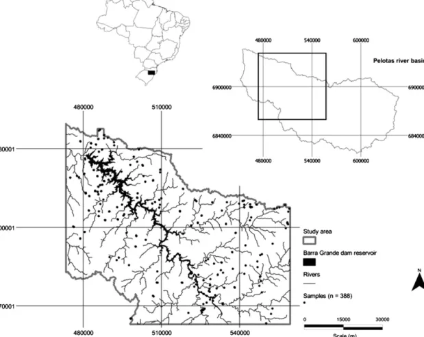
ThefieldsurveywasconductedaroundtheBarraGrandedam
reservoirinsouthernBrazil(Fig.1).LocatedinthePelotasRiver
Basin betweenthe states of SantaCatarina and Rio Grande do
Sul, this reservoir encompasses approximately 90km2, and its
surroundings,delimitedbywatershedboundaries,coveranarea
ofroughly4600km2.Elevationrangesbetween500and1200m
abovesealevel,andtheclimatetypesrangefromCfa(humid
sub-tropical)toCfb(oceanicormarinetemperate),dependingonthe
elevationquota (Köppenclimateclassification).Annual
precipi-tationis1.412mm,andthemeantemperatureis15.2◦C (Maluf,
2000).Topographyvariesfromrollinghighlands(Southern
Brazil-ianPlateau),wherecambisolandalfisolarethemostcommonsoil
classes,tosteepslopesnearthePelotasRiver,wherelithosolis
themostfrequentclass(Potteretal.,2004;sensuBraziliansoil
classificationsystem–SiBCS).
Thevegetationischaracterisedbycontinuousareasof
semi-deciduousforestspredominantlylocatedclosetothePelotasRiver.
Inthehighlands(≥800m),Araucariaforestscoveralargeareathat
isnaturallyfragmentedbygrasslands(Jolyetal.,1999;Klein,1975).
2.2. Targetspecies
Thetime and resourcesavailableallowedthefield sampling
of nine selected species: Araucaria angustifolia (Bertol.) Kuntze
(Araucariaceae), Butia eriospatha (Mart. ex Drude) Becc.
(Are-caceae), Clethra scabra Pers. (Clethraceae), Dicksonia sellowiana
(Presl.)Hook.(Dicksoniaceae),ErythrinafalcataBenth.(Fabaceae),
Maytenus ilicifolia (Schrad.) Planch. (Celastraceae), Myrocarpus
Fig.1. Locationmapofthestudyareaandsamplingsites(UniversalTransverseMercatorcoordinatesystem,Zone22J,southernBrazil).
Endl.(Podocarpaceae)andTrithrinaxbrasiliensisMart(Arecaceae).
ExceptforE.falcata,allofthesespeciespossessthreatcategories,
bothglobally(IUCNRedList)andlocally(RioGrandedoSulStatelist
ofthreatenedspecies).Duetotheintensecommercialexploitation
ofD.sellowiana,thisfernhaditsmarketregulatedbythe
Conven-tiononInternationalTradeinEndangeredSpeciesofWildFauna
andFlora(CITES,AppendixII).Allofthesespeciesareeasily
iden-tifiedinthefield,minimisingsamplingerrors(falseabsences).
2.3. Sampling
Past studies have used standardised abundance estimates
obtainedfromdifferentsurveysorestimatesofabundancefrom
indirectmethods (F-igueiredoandGrelle, 2009;HeandGaston,
2007).Thesemethods,accordingtoAustinandMeyers(1996),can
createanunwantedbias.Incontrast,ourworkwasbasedon
reli-ableoccurrenceandabundancedata.Thesedatawereobtainedby
conductingadetailedfieldsurveyandgermplasmcollection
expe-ditionsforthepurposeofexsituconservationofthetargetspecies.
We randomly sampled 388 georeferenced plots (10m×50m)
aroundtheBarraGrandehydropowerdamreservoir.Ineachplot
wecountedthenumberofindividualsofeachtargetspecieswith
heightgreaterthan1.5m.Topreventorreducetheinfluenceof
topographyinsampling,plotswereallocatedalongdifferent
topo-graphiccontourlevels,similartothosedescribedbyMagnusson
etal.(2005)forrapidsurveysofbiodiversity.
Toavoid anyeffectsofspatialautocorrelation,theminimum
distancebetweenplotswas50m.Thevalueofthisprecautionwas
latervalidatedbyMoran’sIcorrelograms.Allcorrelogramswere
calculatedusingthesoftwareSAMv3.1(Rangeletal.,2010).Forall
targetspecies,thevariationfollowsarandompatternwithasmall
oscillationaroundthezerovalue,whichrepresentstheabsence
ofsignificantautocorrelation(AppendixA;FortinandDale,2005;
LegendreandLegendre,1998).
2.4. Environmentalvariables
Weused15environmentalvariables(directandindirect,sensu
AustinandMeyers,1996)topredictthespatialdistributionofthe
targetspecies(Table1).Allenvironmentalmapshadaspatial
res-olutionof30m.Allspatialdatawerestoredandanalysedusingthe
Table1
Environmentalvariablesusedtopredictthespatialdistributionofthetargetspecies.
Group Variable Soil pHH2O Ca+2+Mg2+* H++Al3−* K+ S2− P+ Totalnitrogen Silt:clayratio* Bulkdensity Topography Elevation(m)* Northness Eastness
Topographicalwetnessindex(TWI) Slope(◦)
Currentvegetation NormalisedDifferenceVegetationIndex(NDVI)
*VariablesexcludedfromanalysisduetohighPearsoncorrelationcoefficient(r)
softwareQuantumGISv.1.5.0(QuantumGISDevelopmentTeam,
2009)anditsinterfacetoGRASS(GRASSDevelopmentTeam,2010).
2.4.1. Topographicvariables
ElevationvalueswereobtainedfromaDigitalElevationModel
(DEM)generatedbytheASTERsensor(ASTERGDEM).Fromthis
DEM,fournewtopographicvariablesweregenerated(northness,
eastness,topographicwetnessindexandslope).(i)Northnessand
eastness(Roberts,1986):theoccurrenceof differentvegetation
physiognomiesisintimatelyconnectedtotheamountofavailable
solarradiation.Inthesouthernhemisphere,placeswitha
north-eastsolarorientationhavegreaterSunexposureandconsequently
ahigherrateofevapotranspiration,resultingintheoccurrenceof
vegetationwithxerophyticcharacteristics.Conversely,slopes
fac-ingsouth–southeast,especiallyduringthewinter,areexposedto
lesssunlight(Kirkpatricketal.,1988;KirkpatrickandNunez,1980).
Toexplorethisrelationship,aspect-modifiedmapswerecreatedin
thisstudy.Themapsindicateatrendtothenorth(northness=cos
[aspect])andeast(eastness=sin[aspect]).Afterthis
transforma-tion,bothvariablesreachedvaluesbetween1and−1,indicating
agradientnorthtosouthandwesttoeast.(ii)Topographic
wet-nessindex(TWI)describesthespatialpatternofsoilwetnessand
isdefinedasafunctionofslope.TWIisobtainedusingthefunction
ln(A/tanˇ),whereAistheupslopedrainingthroughadetermined
pointxgridcellsizeandˇisthepointslope(NetelerandMitasova,
2008;Sørensenetal.,2005).(iii)Slopewasusedtoindicatesoil
depth.A higherdegreeofslopecorresponds toa shallowersoil
depth(PeníˇzekandBor ˚uvka,2006;Tsaietal.,2001).
2.4.2. Soilvariables
Duetothelackofsoilmapsatthespatialresolutionadopted,we
collectedsoilsamplesat381ofoursamplingplots(depth:0–20cm)
and analysed theirchemical and physical properties (Table1).
Owingtologisticalproblemswewerenotabletoanalysesoil
sam-plesfromtheremainingsevensites.Toovercomethis problem,
weperformedaspatialinterpolationofthepropertiesofour381
soilsamples,usingtheregularisedsplinewithtensionalgorithm
(RST;MitasovaandHofierka,1993;MitasovaandMitas,1993),to
coverallthesitesstudied.RSTisarobustandflexiblemethodused
toselectparametersthatcontrolthepropertiesofthe
interpola-tion(tensionandsmoothing).Inaddition,estimatesgeneratedby
RSThaveaccuracysimilartotraditionalgeostatisticalmethods(e.g.
ordinaryanduniversalkriging;seeChaplotetal.,2006formore
details).Thebestinterpolationcontrolparametercombinationwas
selectediterativelyusingcross-validation(leave-one-outmethod;
Tomczak,1998).Toensureaccuracy,weexaminedthedecreasein
rootmeansquareerror(RMSE)andmeandifferencesbetweenthe
observedandpredictedvalues(theclosertozero,thebetterthe
estimate).Inaddition,oursoilmapswerevalidatedusingother,
coarser-scalesoilmapsavailableforthisregion.
2.4.3. Currentvegetationcover
Toestimatecurrentvegetationcover,weusedtheNormalised
DifferenceVegetationIndex(NDVI),obtainedbydividingbands3
(visiblered)and4(nearinfrared)ofLandsat5TM.NDVIvalues
varybetween−1.0and+1.0,andhighpixelvaluesrepresent
plen-tifulvegetation.Toavoidanyeffectsofleafphenologyduringthe
year(forestdeciduousness),weusedLandsat5TMimagescollected
duringsummerinthesouthernhemisphere.
2.5. Dataanalysis
ExceptfortheMoran’sIcorrelogramsdescribedabove,allother
statisticalanalyseswerecarriedoutwithRsoftware(v.2.10.0;R
DevelopmentCoreTeam,2009).
2.5.1. Presence–absencemodels
Generalised Linear Models (GLMs) are the most common
regression methodusedtopredictspecies’spatialdistributions.
AccordingtoMcCarthyandElith(2002),GLMsprovidearigorous
andstatisticallyrobustmethodtopredicttheoccurrence(or
abun-dance) ofspecies.We modelledtheobservedpresence–absence
of each targetspecies withGLM(binomialdistribution,logistic
linkfunction)usingthe15environmentalvariablesdescribedin
Table 1 as predictors. The predictors were selected through a
forward–backward stepwiseprocedure based on
small-sample-size-correctedAkaike’sInformationCriterion(AICc;Burnhamand
Anderson,2002),usingamodifiedversionofthestepAICfunction
oftheRMASSpackage.Variableswerethusaddedtoorremoved
fromthemodelaccordingtohowtheychangeditsAICc;thebest
(orminimaladequate)modelforeach speciesisachievedwhen
novariablecanbeaddedorremovedwithoutanincreaseinAICc.
Stepwiseselectionisausefulandeffectivetooltoinferdistribution
patternsinductivelyfromobserveddata,whennotheoryor
previ-oushypothesesexistabouttheimportanceofeachvariable(Guisan
andZimmermann,2000;Realetal.,2009).
We evaluatedthe models’discriminationcapacity (i.e.,their
abilitytodistinguishpresencefromabsencecases)usingtheArea
under the ReceiverOperating Characteristic (ROC) curve (AUC;
FieldingandBell,1997).AUCvaluesmayvarybetween0and1.
Val-uescloseto0.5indicatethatmodelpredictionsarenobetterthan
random,andAUCvaluesequalto1indicatea100%chanceforthe
modeltocorrectlyclassifyanevent(inourcase,speciespresence
orabsence).AUCvalueslowerthan0.5indicatethatthemodelis
discriminatingpresencesfromabsences,butusingtheinformation
inareversedway(Fawcett,2006).Thenullhypothesisthatthearea
underROCcurveis≤0.5wastestedusingaMann–WhitneyU-test
(MasonandGraham,2002).
Model predictions were alsocompared withthe abundance
datacollectedinthesamesites.UsingSpearman’srankcorrelation
(rho),wetestedtherelationshipbetweenobservedspecies
abun-danceandthepredictedprobabilityofoccurrenceforeachspecies.
Wealsotestedthehypothesis thatifamodelcorrectlypredicts
abundance,ithasahighdiscriminationcapacity(Jiménez-Valverde
etal.,2007).Werepeatedthisanalysisusingonlylocationswith
observedabundance>0assuggestedbyPearceandFerrier(2001).
Wealsoverifiedtherelationshipbetweenmeannumberof
occu-piedsitesperspecies(whichisthesamplesizeforabundance>0)
andabundanceusingaWilcoxonranksumtest(Zar,1999).
2.5.2. Abundancemodels
RegressionmodelsbasedonPoissondistributionsareoftenused
toanalysecountdata(suchasabundance).However,thesedata
areoftenZero-inflated,i.e.,theincidenceofzeros islargerthan
expectedbychance(Ridoutetal.,1998;Welshetal.,1996).Zuur
etal.(2009)describedfivesourcesofzeros,tworelatedtospecies
occupancypatterns(i.e.,thehabitatisnotsuitableandthespecies
is notpresent, orthehabitatis suitablebut is notusedby the
species)andthreerelatedtosamplingerrors(i.e.,designerror,low
speciesdetectability,andsamplingoutsidespecies’habitatrange
–“naughtynaughts”sensuAustinandMeyers(1996)).The
rigor-ousnessofourfieldsurveyandthehighdetectabilityofourtarget
specieswarrantthatoursamplesdonotcontainfalsenegatives
(samplingerrors),sothezeros thatdooccurareonlyrelatedto
patternsofspeciesoccupancy.
Tomodelabundanceweusedthesame15environmental
pre-dictorsdescribedinTable1andtestedthreedifferentalgorithms:
(i) GLM withPoisson (P) and negative binomial (NB)
distribu-tions(GLMPandGLMNB),(ii)Hurdlemodels(HPandHNB,Zeileis
et al., 2008) and (iii) Zero-Inflated Count Data Regression (ZIP
andZINB,respectively).GLMP (standardPoisson)isthesimplest
(variance=mean),butthisassumptionisnotalwaysmetin
prac-ticeduetozero-inflation(variance>mean).Onealternativetodeal
withoverdispersionistheuseofnegative-binomialregressions,
wherevarianceisestimatedasaquadraticfunctionofthemean
(VerHoefandBoveng,2007;LindénandMäntyniemi,2011).
Hurdle models are two-componentclass models capable of
accountingforoverdispersion,orunderdispersion,usingPoisson
(HurdleP)ornegative binomial(HurdleNB)distributions.Hurdle
modelsslacktheassumptionthatzerosandvalues>0comefrom
thesame process (Cameronand Trivedi, 1998).As a first step,
Hurdlemodelsusea truncatedcountcomponent forvalues >0,
assumingthatthesevaluesarisefromtheeffectofconditionsthat
resultinpassingaprobabilitythresholdorzero-hurdle(Cameron
andTrivedi,1998; Gray,2005;Pottsand Elith,2006).Asa
sec-ondstep,aHurdlecomponentmodelszerosvs.non-zerovalues
usingabinomialGLM(Zeileisetal.,2008).Zero-inflatedmodels
aretwo-componentmixturemodelsinwhichzerosaremodelled
asoriginatingfromtwo stochasticprocesses, thebinomial
pro-cessandthecountprocess.SimilartoHurdlemodels,Zero-Inflated
modelsusebinomialGLMtomodeltheprobabilitiesof
measur-ingzeros,andthecountprocessismodelledbyaPoisson(ZIP)or
negativebinomial(ZINB)GLM(Zuuretal.,2009).Thepredictorsof
allabundancemodels(GLM,HurdleandZIPmodels)wereselected
usingthesameAICc-basedapproachappliedtopresence–absence
models(seeSection2.5.1).
Weselectedthebestabundancemodelforeachtargetspecies
usingAICc and evaluatedit withthefollowing fourcriteria:(i)
Pearsoncorrelationcoefficient(r),whichvariesfrom−1to+1and
providesanindicationofagreementbetweenobservedand
pre-dictedabundancevalues(notethataperfectadjustment(r=1)does
notimplyanexact prediction);(ii)Spearman’srankcorrelation
(rho),whichalsovariesfrom−1to+1andprovidesanindication
ofsimilarityinrankbetweenobservedandpredictedabundance
values;(iii)linearregressioncoefficients,whichareobtainedby
fittingasimple linearregression (observedvalues=m(predicted
values)+b;inaperfectlycalibratedmodel,mshouldequal1andb
shouldequal0);and(iv)rootmeansquareerror(RMSE)and
aver-ageerror(AVEerror),bothofwhicharedependentonsamplesize
andmeasuredivergencesbetweenobservedandpredicted
abun-dancevalues(PottsandElith,2006).Confidenceintervals (95%)
foreachevaluatedparameterwerecalculated usingabootstrap
procedure(1000replicates).
3. Results
3.1. Presence–absencemodels
AUCvaluesrangedfrom0.71to0.96andinallcaseswere
sig-nificantlydifferentfrom0.5(Mann–WhitneyU-test,P<0.01;for
detailsaboutenvironmentalvariablesincludedintheGLM
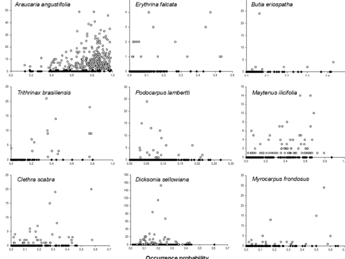
mod-elsseeAppendixB).Overall,therelationshipbetweenobserved
abundanceand occurrence probability waspositive and
statis-ticallysignificant (Table 2 and Fig. 2).When we truncatedthe
abundancedatatoeliminatezeros,theresultsweredifferent.Only
A.angustifolia (whichhadthehighestprevalence) andC.scabra
(witharelativelylowprevalence)retainedsignificantcorrelations
betweenobservedabundanceandprobabilityofoccurrencevalues
(Table2andFig.2).Fortheremainingsevenspecies,the
relation-shipbetweenabundanceand probabilityofoccurrencewasnot
significantwhenunoccupiedsiteswereexcluded.Note,however,
thatthisexclusionofunoccupiedsitesimpliedthatthemean
sam-plesizeforthesespecieswassignificantlysmaller(Mann–Whitney
U-test,P<0.001).
ThecorrelationbetweenAUC(i.e.,modeldiscrimination
capac-ity) and rho (i.e., the rank correlation between occurrence
Table2
Presence–absence model evaluation. Abundance: median and range, P (%): (Prevalence=[truepositives+falsenegatives]/samplesize)×100;rho:Spearman’s rank correlation;AUC: areaunder the receiver operator characteristic curve (Mann–WhitneyU-test).
Targetspecies Abundance P(%) rho rho(Abd>0) AUC
A.angustifolia 4(0–49) 72.42 0.42* 0.17* 0.77** B.eriospatha 0(0–24) 1.55 0.21* 0.39 0.95** C.scabra 0(0–27) 9.79 0.30* 0.32* 0.79** D.sellowiana 0(0–153) 13.40 0.25* 0.02 0.71** E.falcata 0(0–4) 4.38 0.23* 0.16 0.83** M.ilicifolia 0(0–14) 21.13 0.47* 0.08 0.83** M.frondosus 0(0–29) 5.15 0.32* 0.12 0.92** P.lambertii 0(0–24) 5.67 0.18* 0.00 0.73** T.brasiliensis 0(0–21) 4.12 0.32* 0.21 0.96** *P<0.05. **P<0.001.
probability and abundance) was 0.18 (Spearman coefficient,
P=0.63).Therefore,wefoundnoproofthatmodelswithbetter
dis-criminationcapacitywerebetteratpredictingspeciesabundance.
3.2. Abundancemodels
Duetothehighprevalenceofzerocounts(98%),wewerenot
abletomodeltheabundanceofB.eriospatha.BasedonAICcvalues,
HurdleandZero-Inflatedmodels(Poissonornegativebinomial
dis-tributions)werebetterthanGLMwithPoissonornegativebinomial
distributions(Table3).
We could clearly distinguish three groups of species using
abundanceevaluationparameters.(i)C.scabra,D.sellowiana,M.
frondosusandP.lambertiishowedtheworst-fitmodelswiththe
highest values of RMSEand AVEerror (Fig.3).D. sellowiana had
astrongandinconsistentbias(b=1.461andm=0.151),whileC.
scabra,M.frondosusand P.lambertii showedsimilarvalues ofb
(0.230,0.203and0.304,respectively)andm(0.01,0.05and0.00,
respectively).(ii)E.falcata,M.ilicifoliaandT.brasiliensisshowed
accurateabundanceestimates,withbandmequalorclosertozero
andone,respectively(Fig.3).Thesespecieshadrelativelyhigh
val-uesofr(≥0.55)andrho(≥0.33),indicatingthatbothobservedand
predictedabundancemeasuresweresimilarinmagnitude,butnot
similarlyordered(PottsandElith,2006).Also,thesespeciesgave
thesmallestRMSEandAVEerror(Fig.3).(iii)Finally,agroup
com-posedbyonlyA.angustifoliawhichhadconsistentbias(b=1.06and
m=0.83;Fig.3).
3.3. Environmentalcorrelatesofoccurrenceandabundance
SoilpHwasnegatively relatedtotheabundanceofA.
angus-tifolia, C. scabra, D. sellowiana and M. frondosus, and positively
relatedtotheabundanceofT.brasiliensis(Table4).SoilpH
pro-videsanindirectnutrientgradientinthesoil,anditsvaluesdirectly
affect theuptake of K+,S2− and P+ (low or negative ˇ values,
Table3
SelectedabundancemodelsbasedonAICc.ZIP,Zero-InflatedCountDataRegression
withPoissondistribution;ZINB,Zero-inflatedCountDataRegressionwithNegative
Binomialdistribution;HurdleNB,HurdleModelRegressionwithNegativeBinomial
distribution.
Targetspecies Model AICc
A.angustifolia ZINB 2148.84 C.scabra ZINB 347.28 D.sellowiana ZINB 617.37 E.falcata ZINB 144.35 M.ilicifolia HurdleNB 569.96 M.frondosus ZIP 173.67 P.lambertii ZIP 241.48 T.brasiliensis ZINB 158.12
Table4
Variablesincludedintheabundancemodels(countandzerocomponents)obtainedforthestudiedspecies.ˇ,coefficient;S.E.,standarderror;P(z),significanceofthe z-statistictest.
Targetspecies Modelcomponent Variable ˇ S.E. P(z)
A.angustifolia Count pHH2O −0.72 0.14 <0.001 S2− −0.07 0.03 0.03 Eastness 1.82 0.40 <0.001 Slope 0.03 0.01 <0.001 Zero pHH2O 1.33 0.58 0.02 S2− −0.18 0.05 <0.001 Ntotal −11.44 3.75 0.002 Northness 10.44 3.22 <0.001 Eastness 5.95 2.39 0.01 NDVI −5.13 1.76 0.005 Slope −0.18 0.07 0.01 C.scabra Count Constant 58.82 12.63 <0.001 pHH2O −1.27 0.61 0.03 S2− −0.07 0.02 0.003 P+ −0.56 0.16 <0.001 Bulkdensity −17.54 4.23 <0.001 NDVI −20.18 4.00 <0.001 Slope 0.27 0.05 <0.001 S2− −0.13 0.05 0.01 P+ −1.03 0.51 0.04 NDVI −20.63 8.55 0.01 D.sellowiana Count Constant 7.94 3.38 0.02 pHH2O −1.30 0.61 0.03 K+ 1.68 0.61 0.006 Ntotal 6.22 2.81 0.02 TWI −0.05 0.19 0.009 Slope 0.14 0.06 0.01 E.falcata Count Constant −31.89 3.59 <0.001 pHH2O 2.67 0.73 <0.001 K+ −3.46 0.69 <0.001 Ntotal 19.75 4.36 <0.001 Bulkdensity 6.27 1.52 <0.001 Eastness −8.38 2.13 <0.001 Zero K+ −55.17 27.09 0.04 M.ilicifolia Count P + 0.69 0.26 0.007 Northness 2.03 0.88 0.02 Zero Constant −17.60 2.07 <0.001 pHH2O 2.66 0.35 <0.001 S2− 0.08 0.01 <0.001 M.frondosus Count Constant 76.65 13.24 <0.001 K+ 1.09 0.23 <0.001 S2− −0.36 0.06 <0.001 P+ −1.02 0.17 <0.001 Bulkdensity −23.20 3.54 <0.001 Eastness 8.09 0.91 <0.001 Slope 0.13 0.02 <0.001 Zero Constant 673.77 288.92 0.02 pHH2O −42.25 18.68 0.02 K+ −6.83 3.35 0.04 S2− −3.38 1.47 0.02 P+ −2.82 1.30 0.03 Ntotal 89.08 43.27 0.04 Bulkdensity −137.98 59.40 0.02 Eastness 38.07 16.31 0.02 Slope −1.25 0.57 0.03 P.lambertii Count Constant −3.75 1.46 0.01 K+ −2.16 0.47 <0.001 P+ 0.53 0.11 <0.001 Ntotal 4.68 2.31 0.04 Northness 8.88 2.36 <0.001 Eastness −6.21 1.65 <0.001 TWI 0.52 0.08 <0.001 NDVI 9.48 2.00 <0.001 Slope −0.56 0.08 <0.001 Zero P+ 0.91 0.30 <0.001 Northness 12.57 5.23 0.01 Slope −0.55 0.21 0.09 T.brasiliensis Count pHH2O 7.86 2.56 0.002 K+ 5.70 1.20 <0.001 S2− −0.25 0.09 0.06 TWI 0.92 0.19 <0.001 NDVI 6.13 1.60 <0.001 Slope 0.52 0.10 <0.001
Fig.2.Relationshipbetweenoccurrenceprobabilityandtrueabundancevalues(abundance≥0)foreachstudiedspecies.Blackdots,speciesabsence;whitedots,species presence.
Table4)for each species. The occurrence of M. ilicifolia
corre-latedwithsoilpH.However,neitherabundancenoroccurrence
ofP.lambertiiwasaffectedbysoil pH.The abundanceofE.
fal-cata, was positively related to the amount of nitrogen in soil,
whiletheabundanceofP.lambertiiwaspositivelyrelatedto
nitro-gen (Table 4). Northness, eastness, slope and TWI each had a
differentrelationship withthevalues of abundanceand
occur-rence,occasionallyaffectingboth simultaneously(Table4).The
valuesofNDVI,anindirectindicatorofthestageofvegetation
suc-cession(currentvegetationbiomass),werenegativelyrelatedto
theabundanceofC.scabra.OccurrenceofC.scabrawasalso
asso-ciatedwithlowvaluesofNDVI,whileP.lambertiiandT.brasiliensis
werepositivelyrelatedtoNDVI(Table4).
4. Discussion
4.1. Presence–absencemodelsandtheirrelationshipwith
abundance
Becauseoftheneedforreliablespeciesdistributionmodelsto
aidindevelopingconservationstrategies,methodsusedtoassess
modelaccuracyareoneofthemostimportantissues inspecies
distributionmodelling(seee.g.Elithetal.,2006;FieldingandBell,
1997;Maneletal.,2001).Loboetal.(2008)conductedadetailed
descriptionofthedifferentissuesinvolvedwiththemisuseofthe
AUC,which iswidelyusedasameasureofaccuracy ofspecies’
distributionmodels.Onealternativeproposedbytheauthorsisthe
useofabundancedatatovalidatethesemodels.Thisideaisbased
onaninductiverelationship,whereprobabilitiesofoccurrenceare
functionallyrelatedtospeciesabundance(Nielsenetal.,2005).
Pearceand Ferrier(2001)attemptedtousepredicted
proba-bilities of occurrence asa surrogatemethod topredict species
abundance.However,accordingtotheseauthors,therelationship
betweentheprobabilitiesgeneratedbylinearmodelsandobserved
abundanceisweakandrestrictedtoafewspecies.Similarresults
havebeenreportedbyNielsenetal.(2005)andJiménez-Valverde
etal.(2009).Inbothstudies,theprobabilityofoccurrenceisnot
correlatedwithabundancewhenpointswithzeroabundanceare
excludedfromanalysis.PearceandFerrier(2001)suggestthatthe
overallcorrelationbetweenabundanceandprobabilityof
occur-renceisduemostlytothedifferenceinmeanpredictedprobability
betweenoccupiedandunoccupiedsites.However,thefactthatthis
correlationoftendisappearswhenunoccupiedsitesareexcluded
mightalsobedue,atleastinpart,toareductioninsamplesizeand
theconsequentlossofanalyticalpower.Indeed,inourdata,
sam-plesizewashighlysignificantlyreducedwhenunoccupiedsites
wereexcluded (mean occupiedsample size=59.33±86.32; see
“prevalence”inTable2),whichmayhaveimpededthedetection
of significant relationships between abundance and
probabil-ityof occurrence inoccupiedsites. AlsoinPearce andFerrier’s
(2001)study,for59species,therelationshipbetweenabundance
and probability of occurrence (mean sample size=55.49,
stan-darddeviation=47.50)wasnolongersignificantwhenunoccupied
siteswere excluded(meansample size=42.98,standard
devia-tion=38.43).Wefoundthatthemeansamplesizeconsideringonly
occupiedsiteswasalsosignificantlylowerintheirstudy(Wilcoxon
Fig.3.Abundanceevaluationparameters(95%CI).r,Pearsoncorrelationcoefficient;rho,Spearman’srankcorrelation;b,intercept;andm,gradientofthefittedline (observed=b+m(predicted));RMSE,rootmeansquareerror;AVEerror,averageerror.
correlationremainedsignificant(meansamplesize=111.38,
stan-dard deviation=47.31). These results suggest that sample size
mightbeinfluencing thedetectionof anoccupancy–abundance
relationship.
Realetal.(2009)alsoshowedthatpredictionsofGLMsbased
onthepresence–absencedataoftheIberianlynx(Lynxpardinus)
andwildrabbit (Oryctolaguscuniculus)inSpainaresignificantly
correlated with independent abundance data. Even when we
repeatedtheiranalysisexcluding unoccupiedsites,the
correla-tionsremainedsignificantfortheabundanceofrabbit(Kendall’s
Tau-b=0.100,P=0.036,n=300)andlynxin1950(therewereno
zero-abundancedataforthisyear),1965(Tau-b=0.108,P=0.005,
n=355),and1975(Tau-b=0.086,P=0.035,n=315).Onlyinone
case(lynxdatafrom1985)wasthecorrelationnolongersignificant
betweentheirpredictedfavourability and observed abundance,
possibly due to the lower sample size (n=215) when
zero-abundancecellswereexcludedforthisyear.Thisprovidesfurther
supporttotheidea that,givensufficient samplesize,predicted
probabilityofoccurrencemaybearoughindicatorofactualspecies
abundance.
Reconstructing or inferring abundance from species
occur-rencedatacanpotentiallybeanimportanttoolforconservation
planning efforts and species management, especially given the
difficulty of obtaining and analysing abundance data. Current
techniques are oftennot reliable becausethey generate
unsta-ble,low-qualityresults(spuriousestimates;Josephetal.,2009).
Theoccupancy–abundancerelationshipmayadditionallybe
con-ditionedbyecologicalorlife-historytraitsofthemodelledspecies,
asweexposeinthenextsection.Furtherresearchmayprovide
usefulinsightsintothismatter.Inthemeanwhile,andgiventhat
urgentmeasuresareneededtomitigatetheimpactsof
hydroelec-tric powerdamsonthreatenedspecies,we advocatetheuseof
occurrencemodelsassurrogatesforspeciesabundancewhenthe
lattercannotbeobtained.Wedefendthat,givensufficientsample
sizes,probabilityofoccurrencemeasurescannotonlybean
andLoboetal.(2008),butalsoprovideasimpleandinexpensive
alternativefortheabundancemeasureformostspecies.This
alter-nativemethodalsohasgreatpotentialtobeusedinenvironmental
assessment(seealsoAraújoandWilliams,2000;Realetal.,2009).
4.2. Ecologicalconstraintsontheoccupancy–abundance
relationship
Jiménez-Valverdeetal.(2009)suggestthatgeneralistspecies
and those with a high degree of dispersal show positive and
significantrelationshipsbetweenabundance(>0)andthe
proba-bilityofoccurrence.Nielsenetal.(2005)recommendanapproach
basedonorganismlifehistorytoexplaintherelationshipbetween
occurrenceandabundancepatterns,whichisdifferentfromthe
traditionalapproach based onextensiveand exploratoryfitting
exercises. In our study, A. angustifolia and C. scabra were the
only species that exhibited a positive and significant
correla-tionbetweenprobabilitiesofoccurrenceandobservedabundance
whenzero-abundanceplotswereexcludedfromtheanalysis.Both
speciesaretiedtoearlysuccessionalstagesinthestudiedregion
(Duarteetal.,2006;SampaioandGuarino,2007),andseveral
stud-iesindicatethatA.angustifoliaisabletoadvanceforestexpansion
overnaturalgrasslandsandcolonisenewareasofgrasslandsinthe
highlandsofsouthernBrazil(Duarteetal.,2006).Furthermore,the
seedsofA.angustifoliaaredispersedbybirdsandsmallmammals
(Anjos,1991;IobandVieira,2008),whereasC.scabra’sseedsare
wind-dispersedandcanthustravelgreaterdistances.
Another interesting case is that of subtropical palms, B.
eriospathaand T.brasiliensis,which are gregarious specieswith
densebutsporadicpopulationsinthestudyarea.Becauseofthe
importanceoffibreand thehighnutritionalvalueof thefruits,
bothspecieswereinfluencedbyancienthumaninhabitantsofthe
region.Thepopulationofthesespecieswaspurposefullydispersed
bynativesandEuropeansettlers,whograzedlivestockforcenturies
intheareawestudied(Reitzetal.,1974).Pasthuman-mediated
dispersioncanaffectthecurrentpatternsofplantdistribution,
cre-atingartificiallyclusteredpopulationsthatareoftenunnoticedin
extensiveexploratorymodel-fittingexercises.Althoughthis
his-toryofplantmanipulationisimportant,ithasrarelybeenincluded
instudiesofspeciesdistributions(Lutolfetal.,2009).
Therelativelylowstrengthofthecorrelationbetweenpredicted
occurrenceprobabilitiesandobservedabundance(<0.5inallcases)
couldalsobeduetobioticinteractionsnotincludedinthe
occur-rencemodels.Austinetal.(1990)andGuisanandThuiller(2005),
forexample,suggestedthattheresponsecurveofaspeciesalong
anenvironmentalgradientcanbeseriouslyconstrainedby
inter-actionwithbioticfactors.Thishypothesiswasrecentlytestedby
Heikkinenetal.(2007)and Ritchieetal.(2009),usingdifferent
organisms,andtheybothfoundsimilarresults.Whendatarelated
tointerspecificcompetitorswereincorporatedintomodels,species
predictionsweresignificantly improved. In addition, this effect
likely plays a role in the relationship betweenoccurrence and
abundance,obscuringthetruerelationshipbetweenoccupiedarea
andabundance.Ritchieetal.(2009)confirmedthisidea
demon-stratingthatthepredictedabundanceofwallaroosandkangaroos
wasimprovedwiththeadditionoftheoccurrenceandabundance
ofinterspecificcompetitorsintothemodels.However,obtaining
thesedataisdifficultandmodelpractitionersmustcontinuetouse
mostlyabioticfactors(Barbosaetal.,2009;ElithandLeathwick,
2009).
4.3. Abundancemodels
Ingeneral,Zero-InflatedmodelsperformedbetterthanHurdle
models.Thisresultiscontrarytootherempiricalstudiesonboth
realpopulations(PottsandElith,2006)andtheoreticalstudieswith
pseudo-populations(MillerandMiller,2008),suggestingthat
Hur-dlemodelsgenerallyperform betterthanZero-Inflatedmodels.
Becausethetechniquesusedinthisstudytomodelabundancedeal
differentlywithzeros,theresultscanbeinterpretedinseveralways
(PottsandElith,2006;Zuuretal.,2009).Two-partmodelling
tech-niques,suchasGLMHurdlemodels,analyseabundancedatainthe
followingtwosteps:(i)zerovs.non-zerovaluesaremodelledwitha
logisticregression(binomialdistribution),and(ii)non-zero
obser-vationsaremodelledwithatruncatedPoissonornegative-binomial
regression.Mixedtechniques,suchasZero-Inflatedmodels,
clas-sifyzerosasoriginatingfromtwodifferentprocesses,binomialand
countprocesses(Zuuretal.,2009).InterpretingHurdlemodelsis
simplerthaninterpreting Zero-Inflatedmodels(Pottsand Elith,
2006),but,accordingtoWelshetal.(2000),mixedmodels
pro-videabettertoolwhenthereisoverdispersionandalargenumber
oftruezeros,aswasthecasewithourdata.
4.4. Variablesrelatedtospeciesoccurrenceandabundance
Ourmainobjectivewiththefittedmodelswastopredictspecies’
distributionandabundanceratherthantotesttheeffectsof
dif-ferent ecological drivers onspecies occurrence and abundance.
However, we can draw some conclusions about the ecological
factorsthatareassociatedtotheanalysedspecies’distributions.
AccordingtoBarrowsetal.(2005),environmentalmanagersmust
understand the anthropogenic and environmental factors that
influencetheoccurrenceandabundanceofspecies.Withthis
infor-mation,managerscanemployadaptivemanagementstrategiesto
maintainviablepopulationsofdesiredspecies.Overall,occurrence
andabundanceofstudiedspeciesaredetermined,tosomeextent,
bydifferentsuitesofenvironmentalvariables.Regardlessof
organ-ismtype,thispatternhasbeenwidelyreported(Heinanenetal.,
2008;Illánetal.,2010;Truscottetal.,2008),suggestingthatbiotic
and abioticeventsassociated withplantestablishment maybe
differentthanthoseinfluencingtheirabundance(Truscottetal.,
2008).
Herewehighlighttherelationshipbetweentheabundanceof
E.falcataandtotalnitrogenavailability.Abundance(countmodel
component)ofE.falcatawasnegativelyrelatedtolowsoil
nitro-genvalues.Thisspecies,alongwithothersofthesamegenus,are
generallyabletoproducenitrogen-fixingrootnodules(Fariaetal.,
1984,1989;Schimannetal.,2008).However,itsrootshaveaunique
strategytoacquiresoilnitrogen.Theroots donotexploit
avail-ablenitrogeninthesoil,andinsteadusenitrogenintheleaflitter
(ChesneyandVasquez,2007;Payanetal.,2009onE.poeppigianain
agroforestrysystems),anenvironmentalvariablethatwasanalysed
inourstudy.Conversely,M.frondosus,anotherFabaceaespecies,
wasnot reportedtoproducenitrogen-fixingnodules (Allenand
Allen,1981;Fariaetal.,1984).
5. Conclusionsandfutureapplications
Ourstudyisthefirsttoapplyamacroecologicalapproachto
supportinsituandexsituplantconservationpracticesinaregion
affectedbyahydropowerdamreservoir.CurrentlyinBrazil,
Envi-ronmentalImpactAssessment(EIA)andStrategicEnvironmental
Assessment (SEA) methods require costly and time-consuming
fieldsurveys(floristicandphytosociologicalstudies), often
con-ductedbyprofessionalswithanincompleteunderstandingofthe
extreme diversity of Brazilian flora. As a result, these surveys
oftenproducelow-quality,inapplicabledatathataresusceptibleto
environmentalerror.Despitemethodologicallimitations,i.e.,low
(althoughsignificant)correlationbetweenpredictedprobabilityof
occurrenceandobservedabundance,andapossibledependenceon
Brazilcouldprofitfromusingspeciesdistributionmodelstopredict
futureimpactsandplanlandscapemanagementstrategiesand
mit-igationactions.Thisapproachisquickerandlessexpensivethanthe
currentapproach,althoughthismethoddoesrequirestafftraining
indatacollectionandanalysis.
Aneffectivewaytoorganisedatacollectionistocombinethe
gradsect methodproposed by Austin and Heyligers (1989) and
Wesselsetal. (1998)withtherapidassessmentsurveymethod
usedinthisstudyanddescribedbyMagnussonetal.(2005).For
example,insteadofmeasuringtheheightand diameterof each
treespecies within plots, we record onlythe presence of each
speciesingeoreferencedplots.Austinand Heyligers(1989)and
AustinandMeyers(1996)supporttheviewthat formost
envi-ronmentalgoals,includingspeciesnichemodelling,representative
samplesaremoreimportantthanaccuratebasalareaestimations,
whichisthemethodcurrentlyusedinthepreparationofEIA/SEA
inBrazil.Eveninasituationwherefieldsurveysarenotperformed,
presence-onlydataobtainedfromherbariumormuseum
collec-tionsareviablealternatives.Evenwithacoarseresolution,they
canproducepertinentinformation forthedevelopmentof
fine-scalespeciesconservationplanning(Araújo,2004;Barbosaetal.,
2003,2010).
Evenweakly,theoccupancy–abundancerelationshipcan
opti-mise ex situ conservation actions in similar situations. Based
onspeciesdistributionmodelsbuiltwithpresence–absencefield
dataobtainedin rapidand systematicbiodiversityassessments,
we can be able to, a priori, define the rare species set using
occupancy–abundance relationships (Flather and Sieg, 2006).
Regardlessof threatlevels,we canconcentrategermplasm
col-lectionefforts,atafirstglance,onlocallyrarespecieswithlow
abundanceandnarrowareaof occurrence,suchasB.eriospatha
andT. brasiliensis.In asecond step,speciesdistributionmodels
canbeusedasaguidetodefinethemostsuitableareasto
col-lectgermplasmsamplesoftheselectedspecies.Thisapproachis
lessmoneyandtime-consumingandcanaccelerateconservation
actionsinlandscapessubmittedtostronganthropogenicimpacts,
likehydroelectricpowerdamreservoirs.Practicalexamplesofthis
applicationof distributionmodels asa guideto definesuitable
areastocollectspecies germplasmsampleswerefirstdescribed
byJonesetal.(1997)andfollowedbyJarvisetal.(2003,2005a,b),
Villordonetal.(2006)andRamírez-Villegasetal.(2010).However,
inallthesepreviousexamplesauthorsusedpresence-onlymodels
toguidegermplasmcollectingexpeditionsofcropwildrelatives
(i.e.,peanut,potato,pepper)onalargescale.
Themereoccurrenceofonespeciesisnotsufficienttoensure
thepersistenceofaviablepopulationwithinasystemofprotected
areas(Barrowsetal.,2005).Asystemofprotectedareasshould
containsamplesofthelargestpossiblenumberoflocalecosystems,
therebymaintainingtheecologicalprocessesoftheseecosystems
(Australia,1997).Analternativetoaccomplishthisgoalwouldbeto
integrateinformationaboutspeciesoccurrence(orabundance)and
regionallanduseinaninteractivedecision-makingsystem.This
methodwouldensuretheconservationofviablesamplesin
dif-ferentecosystemsoccurringintheregionofinterest(Ferrieretal.,
2002).
Acknowledgments
Thefield workwassupportedby EmbrapaRecursos
Genéti-coseBiotecnologia.E.S.G.G.wassupportedbyBrazilianNational
CouncilforScientificandTechnologicalDevelopment(CNPq;proc.
140712/2007-0)andCoordenac¸ãodeAperfeic¸oamentodePessoal
deNívelSuperior(CAPES;proc.2298/09-0)scholarships.A.M.B.is
supportedbyaPost-DoctoralFellowship(SFRH/BPD/40387/2007)
fromFundac¸ãoparaaCiênciaeaTecnologia(Portugal).The“Rui
Nabeiro”BiodiversityChairisfundedbyDeltaCafésandanFCT
project (PTDC/AAC-AMB/098163/2008). We are grateful to A.A.
Santos,M.B.Sampaio,J.A.Santosandotherswhohelpedwithfield
work.M.B.Araújo,D.L.M.Vieira,A.B.Sampaio,F.S.Rocha,P.R.Vieira
andR.L.L.Orihuelahelpedwithimportantsuggestions.Wearealso
gratefultoC.Scherberwhokindlyprovidedthescriptforstepwise
modelselectionwithAICc.
AppendixA. Supplementarydata
Supplementarydataassociatedwiththisarticlecanbefound,in
theonlineversion,atdoi:10.1016/j.ecolmodel.2012.01.007.
References
Albert,C.H.,Thuiller,W.,2008.Favourabilityfunctionsversusprobabilityof pres-ence:advantagesandmisuses.Ecography31,417–422.
Allen,O.N.,Allen,E.K.,1981.TheLeguminosae:ASourceBookofCharacteristics, Uses,andNodulation,1sted.TheUniversityofWisconsinPress,Madison. Alves,T.P.,Fontoura,N.F.,2009.Statisticaldistributionmodelsformigratoryfishin
Jacuibasin,SouthBrazil.Neotrop.Ichthyol.7,647–658.
Anjos,L.,1991.OcicloanualdeCyanocoraxcaeruleusemflorestadearaucária (Passeriformes:Corvidae).Ararajuba2,19–23.
Araújo,M.B.,2004.Matchingspecieswithreserves–uncertaintiesfromusingdata atdifferentresolutions.Biol.Conserv.118,533–538.
Araújo,M.B.,Williams,P.H.,2000.Selectingareasforspeciespersistenceusing occurrencedata.Biol.Conserv.96,331–345.
Austin,M.P.,Heyligers,P.C.,1989.Measurementoftherealizedqualitativeniche: environmentalnichesoffiveEucalyptusspecies.Biol.Conserv.50,13–32. Austin,M.P.,Meyers,J.A.,1996.Currentapproachestomodellingtheenvironmental
nicheofeucalypts:implicationformanagementofforestbiodiversity.Forest Ecol.Manag.85,95–106.
Austin,M.P.,Nicholls,A.O.,Margules,C.R.,1990.Measurementoftherealized qual-itativeniche:environmentalnichesoffiveEucalyptusspecies.Ecol.Monogr.60, 161–177.
AustraliaCo.,1997NationallyAgreedCriteriafortheEstablishmentofa Compre-hensive,AdequateandRepresentativeReserveSystemforForestinAustralia. AReportbytheJointANZECC/MCFFANationalForestPolicyStatement Imple-mentationSub-committee.
Barbosa,A.M.,Real,R.,Olivero,J.,Vargas,J.M.,2003.Otter(Lutralutra)distribution modellingattworesolutionscalessuitedtoconservationplanningintheIberian Peninsula.Biol.Conserv.114,377–387.
Barbosa,A.M.,Real,R.,Vargas,J.M.,2009.Transferabilityofenvironmental favoura-bilitymodelsingeographicspace:thecaseoftheIberiandesman(Galemys pyrenaicus)inPortugalandSpain.Ecol.Model.220,747–754.
Barbosa,A.M.,Real,R.,Vargas,J.M., 2010.Useof coarse-resolutionmodelsof species’distributionstoguidelocalconservationinferences.Conserv.Biol.24, 1378–1387.
Barrows,C.W.,Swartz,M.B.,Hodges,W.L.,Allen,M.F.,Rotenberry,J.T.,Li,B.L.,Scott, T.A.,Chen,X.W.,2005.Aframeworkformonitoringmultiple-species conserva-tionplans.J.WildlifeManage.69,1333–1345.
Blackburn,T.M.,Gaston,K.J.,2009.Sometimestheobviousanswer istheright one:aresponseto‘Missingtherarest:isthepositiveinterspecific abundance-distributionrelationshipatrulygeneralmacroecologicalpattern?’.Biol.Lett.5, 777–778.
Brown,J.H.,1984.Ontherelationshipbetweenabundanceanddistributionof species.Am.Nat.124,255–279.
Burnham,K.P.,Anderson,D.R.,2002.ModelSelectionandMultimodelInference:A PracticalInformation–TheoreticApproach.Springer,NewYork.
Cameron,A.C.,Trivedi,P.K.,1998.RegressionAnalysisofCountData.Cambridge, NewYork,p.432.
Cayuela,L.,Golicher,D.J.,Newton,A.C.,Kolb,M.,Albuquerque,F.Sd.,Arets,E.J.M.M., Alkemade,J.R.M.,Perez,A.M.,2009.Speciesdistributioninthetropics:problems, potentialities,andtheroleofbiologicaldataforeffectivespeciesconservation. Trop.Conserv.Sc.2,319–352.
Chaplot,V.,Darboux,F.,Bourennane,H.,Leguedois,S.,Silvera,N.,Phachomphon,K., 2006.Accuracyofinterpolationtechniquesforthederivationofdigital eleva-tionmodelsinrelationtolandformtypesanddatadensity.Geomorphology77, 126–141.
Chen,G.,Kéry,M.,Zhang,J.,Ma,K.,2009.Factorsaffectingdetectionprobabilityin plantdistributionstudies.J.Ecol.97,1383–1389.
Chesney,P.,Vasquez,N.,2007.Dynamicsofnon-structuralcarbohydratereserves inprunedErythrinapoeppigianaandGliricidiasepiumtrees.Agroforest.Syst.69, 89–105.
Duarte,L.D.S.,Machado,R.E.,Hartz,S.M.,Pillar,V.D.,2006.Whatsaplingscantellus aboutforestexpansionovernaturalgrasslands.J.Veg.Sci.17,799–808. Elith,J.,Graham,C.H.,Anderson,R.P.,Dudik,M.,Ferrier,S.,Guisan,A.,Hijmans,
R.J.,Huettmann,F.,Leathwick,J.R.,Lehmann,A.,Li,J.,Lohmann,L.G.,Loiselle, B.A.,Manion,G.,Moritz,C.,Nakamura,M.,Nakazawa,Y.,Overton,J.M.,Peterson, A.T.,Phillips,S.J.,Richardson,K.,Scachetti-Pereira,R.,Schapire,R.E.,Soberón,J.,
Williams,S.,Wisz,M.S.,Zimmermann,N.E.,2006.Novelmethodsimprove pre-dictionofspecies’distributionsfromoccurrencedata.Ecography29,129–151. Elith,J.,Leathwick,J.R.,2009. Speciesdistribution models:ecological explana-tionandpredictionacrossspaceandtime. Annu.Rev.Ecol.Evol.Syst.40, 677–697.
Faria,B.S.M.,Franco,A.A.,Jesus,R.M.,Menandro,M.S.,Baitello,J.B.,Mucci,E.S.F., Döbereiner,J.,Sprent,J.I.,1984.Newnodulatinglegumetreesfromsouth-east Brazil.NewPhytol.98,317–328.
Faria,B.S.M.,Lewis,G.P.,Sprent,J.I.,Sutherland,J.M.,1989.Occurrenceofnodulation intheLeguminosae.NewPhytol.111,607–619.
Fawcett,T.,2006.AnintroductiontoROCanalysis.PatternRecogn.Lett.27,861–874. Ferrier,S.,Watson,G.,Pearce,J.,Drielsma,M.,2002.Extendedstatisticalapproaches tomodellingspatialpatterninbiodiversityinnortheastNewSouthWales.I. Species-levelmodelling.Biodivers.Conserv.11,2275–2307.
Fielding,A.H.,Bell,J.F.,1997.Areviewofmethodsfortheassessmentofprediction errorsinconservationpresence/absencemodels.Environ.Conserv.24,38–49. Figueiredo,M.S.L.,Grelle,C.E.V.,2009.Predictingglobalabundanceofathreatened
speciesfromitsoccurrence:implicationsforconservationplanning.Divers. Dis-trib.15,117–121.
Flather,C.H.,Sieg,C.H.,2006.Speciesrarity:definition,causes,andclassification.In: Raphael,M.G.,Molina,R.(Eds.),ConservationofRareorLittle-knownSpecies: Biological,Social,andEconomicConsiderations.IslandPress,Washington. Fortin,M.J.,Dale,M.,2005.SpatialAnalysis:AGuideforEcologists,1sted.Cambridge
UniversityPress,Cambridge.
Gaston,K.J.,Blackburn,T.M.,Greenwood,J.J.D.,Gregory,R.D.,Quinn,R.M.,Lawton, J.H.,2000.Abundance–occupancyrelationships.J.Appl.Ecol.37,39–59. Gray,B.R.,2005.Selectingadistributionalassumptionformodellingrelative
densi-tiesofbenthicmacroinvertebrates.Ecol.Model.,1–12.
Gu,W.,Swihart,R.K.,2004.Absentorundetected?Effectsofnon-detectionofspecies occurrenceonwildlife-habitatmodels.Biol.Conserv.116,195–203.
Guisan,A.,Thuiller,W.,2005.Predictingspeciesdistribution:offeringmorethan simplehabitatmodels.Ecol.Lett.8,993–1009.
Guisan,A.,Zimmermann,N.E.,2000.Predictivehabitatdistributionmodelsin ecol-ogy.Ecol.Model.135,147–186.
He,F.,Gaston,K.J.,2000.Occupancy–abundancerelationshipsandsamplingscale. Ecography23,503–511.
He,F.,Gaston,K.J.,2007.Estimatingabundancefromoccurrence:an underdeter-minedproblem.Am.Nat.170,655–659.
Heikkinen,R.K.,Luoto,M.,Virkkala,R.,Pearson,R.G.,Korber,J.H.,2007.Biotic inter-actionsimprovepredictionofborealbirddistributionsatmacro-scales.Global Ecol.Biogeogr.16,754–763.
Heinanen,S.,Ronka,M.,vonNumers,M.,2008.Modellingtheoccurrenceand abun-danceofacolonialspecies,thearcticternSternaparadisaeainthearchipelago ofSWFinland.Ecography31,601–611.
Holt,A.R.,Gaston,K.J.,He,F.,2002.Occupancy-abundancerelationshipsandspatial distribution:areview.BasicAppl.Ecol.3,1–13.
Illán,J.G.,Gutierrez,D.,Wilson,R.J.,2010.Thecontributionsoftopoclimateand landcovertospeciesdistributionsandabundance:fine-resolutiontestsfora mountainbutterflyfauna.GlobalEcol.Biogeogr.19,159–173.
Iob,G.,Vieira,E.M.,2008.SeedpredationofAraucariaangustifolia(Araucariaceae) intheBrazilianAraucariaForest:influenceofdepositionsiteandcomparative roleofsmalland‘large’mammals.PlantEcol.198,185–196.
Jarvis,A.,Ferguson,M.E.,Williams,D.E.,Guarino,L.,Jones,P.G.,Stalker,H.T.,Valls, J.F.M.,Pittman,R.N., Simpson,C.E.,Bramel,P.,2003. Biogeographyofwild Arachis:assessingconservationstatusandsettingfuturepriorities.CropSci.43, 1100–1108.
Jarvis, A., Williams, K., Williams, D.,Guarino, L., Caballero, P.J.,Mottram, G., 2005a. UseofGIS for optimizinga collecting missionfor rarewild pep-per(CapsicumflexuosumSendtn.)inParaguay.Genet.Resour.CropEval.52, 671–682.
Jarvis,A.,Yeaman,S.,Guarino,L.,Tohme,J.,2005b.Theroleofgeographicanalysis inlocating,understanding,andusingplantgeneticdiversity.MethodsEnzymol. 395,279–296.
Jiménez-Valverde,A.,Diniz,F.,deAzevedo,E.B.,Borges,P.A.V.,2009.Species distri-butionmodelsdonotaccountforabundance:thecaseofarthropodsonTerceira Island.Ann.Zool.Fennici46,451–464.
Jiménez-Valverde,A.,Ortuno,V.M.,Lobo,J.M.,2007.Exploringthedistributionof Sterocoraxortuno,1990(Coleoptera,Carabidae)speciesintheIberianpeninsula. J.Biogeogr.34,1426–1438.
Joly,C.A.,Aidar,M.P.M.,Klink,C.A.,McGrath,D.G.,Moreira,A.G.,Moutinho,P., Nep-stad,D.C.,Oliveira,A.A.,Pott,A.,Rodal,M.J.N.,Sampaio,E.V.S.B.,1999.Evolution oftheBrazilianphytogeographyclassificationsystems:implicationsfor biodi-versityconservation.Cienc.Cult.51,331–348.
Jones,P.G.,Beebe,S.E.,Tohme,J.,Galwey,N.W.,1997.Theuseofgeographical informationsystemsinbiodiversityexplorationandconservation.Biodivers. Conserv.6,947–958.
Joseph,L.N.,Elkin,C.,Martin,T.G.,Possingham,H.P.,2009.Modelingabundance usingN-mixturemodels:theimportanceofconsideringecologicalmechanisms. Ecol.Appl.19,631–642.
Kirkpatrick, J.B., Fensham, R.J., Nunez, M., Bowman, D.M.J.S., 1988. Vegetation–radiation relationships in the wet–dry tropics: granite hills innorthernAustralia.Vegetatio76,103–112.
Kirkpatrick,J.B.,Nunez,M.,1980.Vegetation–radiationrelationshipsin mountain-ousterrain:eucalypt-dominatedvegetationintheRisdonHills,Tasmania.J. Biogeogr.7,197–208.
Klein,R.M.,1975.SouthernBrazilianphytogeographicfeaturesandtheprobable influenceofupperquaternaryclimaticchangesinthefloristicdistribution.Bol. Parana.Geocienc.33,67–88.
Komonen,A.,Paivinen,J.,Kotiaho,J.S.,2009.Missingtherarest:isthepositive inter-specificabundance–distributionrelationshipatrulygeneralmacroecological pattern.Biol.Lett.5,492–494.
Kotiaho,J.S.,Komonen,A.,Paivinen,J.,2009.Ontheobviouspositiveinterspecific relationshipbetweenabundanceanddistribution:areplytoBlackburnand Gaston.Biol.Lett.5,779–780.
Legendre,P.,Legendre,L.,1998.NumericalEcology,2nded.ElsevierScienceB.V., Amsterdam.
Lindén,A.,Mäntyniemi,S.,2011.Usingthenegativebinomialdistributiontomodel overdispersioninecologicaldata.Ecology,1414–1421.
Lobo,J.M.,Jiménez-Valverde,A.,Real,R.,2008.AUC:amisleadingmeasureofthe per-formanceofpredictivedistributionmodels.GlobalEcol.Biogeogr.17,145–151. Lutolf,M.,Guisan,A.,Kienast,F.,2009.Historymattersrelatingland-usechangeto
butterflyspeciesoccurrence.Environ.Manage.43,436–446.
Magnusson,W.E.,Lima,A.P.,Luizão,R.,Costa,F.R.C.,Castilho,C.V.,Knupp,V.F.,2005. RAPELD,amodificationoftheGentrymethodforbiodiversitysurveysin long-termecologicalresearchsites.Biot.Neotrop.5,19–24.
Maluf,J.R.T.,2000.Novaclassificac¸ãoclimáticadoEstadodoRioGrandedoSul.Rev. Bras.Agrometeorol.8,141–150.
Manel,S.,Williams,H.C.,Ormerod,S.J.,2001.Evaluatingpresence–absencemodels inecology:theneedtoaccountforprevalence.J.Appl.Ecol.38,921–931. Mason,S.J.,Graham,N.E.,2002.Areasbeneaththerelativeoperating
characteris-tics(ROC)andrelativeoperatinglevels(ROL)curves:statisticalsignificanceand interpretation.Quart.J.Roy.Meteorol.Soc.128,2145–2166.
McCarthy,M.A.,Elith,J.,2002.Speciesmappingforconservation.GapAnal.Bull.2, 50–57.
Miller,J.M.,Miller,M.D.,2008.Nozeroleftbehind:comparingthefitfor zero-inflationmodelsasafunctionofskewandproportionofzeros.InterStat11, 35.
Mitasova,H.,Hofierka,J.,1993.Interpolationbyregularizedsplinewithtension:II. Applicationtoterrainmodelingandsurfacegeometryanalysis.Math.Geol.25, 656–669.
Mitasova,H.,Mitas,L.,1993.Interpolationbyregularizedsplinewithtension:I. Theoryandimplementation.Math.Geol.25,641–655.
Neteler,M.,Mitasova,H.,2008.OpenSourceGIS:AGRASSGISApproach,3rded. Springer,NewYork.
Nielsen, S.E., Johnson, C.J., Heard, D.C., Boyce, M.S., 2005. Can models of presence–absencebeusedtoscaleabundance?Twocasestudiesconsidering extremesinlifehistory.Ecography28,197–208.
Parolo,G.,Rossi,G.,Ferrarini,A.,2008.Towardimprovedspeciesnichemodelling: ArnicamontanaintheAlpsasacasestudy.J.Appl.Ecol.45,1410–1418. Payan,F.,Jones,D.L.,Beer,J.,Harmand,J.M.,2009.Soilcharacteristicsbelow
Ery-thrinapoeppigianainorganicandconventionalCostaRicancoffeeplantations. Agroforest.Syst.76,81–93.
Pearce,J.,Ferrier,S.,2001.Thepracticalvalueofmodellingrelativeabundanceof speciesforregionalconservationplanning:acasestudy.Biol.Conserv.98,33–43. Peníˇzek,V.,Bor ˚uvka,L.,2006.Soildepthpredictionsupportedbyprimaryterrain
attributes:acomparisonofmethods.PlantSoilEnviron.52,424–430. Potter,R.O.,Carvalho,A.M.,Flores,C.A.,Bognola,I.,2004.SolosdoEstadodeSanta
Catarina.Bol.Pesquisa,46.EmbrapaSolos.
Potts,J.M.,Elith,J.,2006.Comparingspeciesabundancemodels.Ecol.Model.1999, 153–163.
Pulliam,H.R.,2000.Ontherelationshipbetweennicheanddistribution.Ecol.Lett., 349–361.
Ramírez-Villegas,J.,Khoury,C.,Jarvis,A.,Debouck,D.G.,Guarino,L.,2010.Agap analysismethodologyforcollectingcropgenepools:acasestudywithPhaseolus beans.PLoSOne10,1–18.
Rangel,T.F.,Diniz,J.A.F.,Bini,L.M.,2010.SAM:acomprehensiveapplicationfor spatialanalysisinmacroecology.Ecography33,46–50.
Real,R.,Barbosa,A.M.,Rodriguez,A.,Garcia,F.J.,Vargas,J.M.,Palomo,L.J.,Delibes,M., 2009.Conservationbiogeographyofecologicallyinteractingspecies:thecaseof theIberianlynxandtheEuropeanrabbit.Divers.Distrib.15,390–400. Reitz,R.,1974.Palmeiras.In:ItajaíHerbárioBarbosaRodrigues.
Ridout,M.,Demétrio,C.G.B.,Hinde,J.,1998.Modelsforcountdatawithmanyzeros. In:InternationalBiometricConference,CapeTown,pp.1–13.
Ritchie,E.G.,Martin,J.K.,Johnson,C.N.,Fox,B.J.,2009.Separatingtheinfluences ofenvironmentandspeciesinteractionsonpatternsofdistributionand abun-dance:competitionbetweenlargeherbivores.J.Anim.Ecol.78,724–731. Roberts,D.W.,1986.Ordinationonthebasisoffuzzysettheory.PlantEcol.66,
123–131.
Rodríguez,J.P.,Brotons,L.,Bustamante,J.,Seoane,J.,2007.Theapplicationof pre-dictivemodellingofspeciesdistributiontobiodiversityconservation.Divers. Distrib.13,243–251.
Sampaio,M.B.,Guarino,E.S.G.,2007.Efeitosdopastoreionaestrutura popula-cionaldeplantasemfragmentosdeFlorestaOmbrófilaMista.Rev.Árvore31, 1035–1046.
Schimann,H.,Ponton,S.,Hattenschwiler,S.,Ferry,B.,Lensi,R.,Domenach,A.M., Roggy,J.C.,2008.Differingnitrogenusestrategiesoftwotropicalrainforest latesuccessionaltreespeciesinFrenchGuiana:evidencefromN-15natural abundanceandmicrobialactivities.SoilBiol.Biochem.40,487–494. Skagen,S.K.,YackelAdams,A.A.,2011.Potentialmisuseofaviandensityasa
Soberón,J.,Peterson,A.T.,2005.Interpretationofmodelsoffundamentalecological nichesandspecies’distributionalareas.Biodivers.Inform.2,1–10.
Sørensen,R.,Zinko,U.,Seibert,J.,2005.Onthecalculationofthetopographicwetness index:evaluationofdifferentmethodsbasedonfieldobservations.Hydrol.Earth Syst.Sci.2,1807–1834.
Tomczak,M., 1998.Spatial interpolationandits uncertaintyusingautomated anisotropic inverse distance weighting (IDW) – cross-validation/Jackknife approach.J.Geogr.Inform.Decis.Anal.2,18–30.
Truscott,A.M.,Palmer,S.C.F.,Soulsby,C.,Hulme,P.E.,2008.Assessingthe vulnerabil-ityofriparianvegetationtoinvasionbyMimulusguttatus:relativeimportanceof bioticandabioticvariablesindeterminingspeciesoccurrenceandabundance. Divers.Distrib.14,412–421.
Tsai,C.,Chen,Z.,Duh,C.,Horng,F.,2001.Predictionofsoildepthusinga soil-landscaperegressionmodel:acasestudyonforestsoilsinSouthernTaiwan. Proc.Natl.Sci.Counc.ROC[B]25,34–39.
VanDerWal,J.,Shoo,L.P.,Johnson,C.N.,Williams,S.E.,2009.Abundanceandthe environmentalniche:environmentalsuitabilityestimatedfromnichemodels predictstheupperlimitoflocalabundance.Am.Nat.174,282–291.
VanHorne,B.,1983.Densityasamisleadingindicatorofhabitatquality.J.Wildlife Manage.,893–901.
VerHoef,J.M.,Boveng,P.L.,2007.Quasi-Poissonvs.negative-binomialregression: howshouldwemodeloverdispersedcountdata.Ecology88,2766–2772. Verbek, W.C.E.P., Van der Velde, G., Esselink, H., 2010. Explaining
abundance–occupancy relationships in specialists and generalists: a case studyonaquaticmacroinvertebratesinstandingwaters. J.Anim.Ecol.79, 589–601.
Villordon,A.,Njuguna,W.,Gichuki,S.,Ndolo,P.,Kulembeka,H.,Jeremiah,S.C., LaBonte,D.,Yada,B.,Tukamuhabwa,P.,Mwanga,R.O.M.,2006.UsingGIS-based toolsanddistributionmodelingtodeterminesweetpotatodocumentation pri-oritiesinSub-SaharanAfrica.Hortscience41,1377–1381.
Welsh,A.H.,Cunningham,R.B.,Chambers,R.L.,2000.Methodologyforestimatingthe abundanceofrareanimals:seabirdnestingonNorthEastHeraldCay.Biometrics 56,22–30.
Welsh,A.H.,Cunningham,R.B.,Donnelly,C.F.,Lindenmayer,D.B.,1996.Modelling theabundanceofrarespecies:statisticalmodelsforcountswithextrazeros. Ecol.Model.88,297–308.
Wessels,K.J.,VanJaarsveld,A.S.,Grimbeek,J.D.,VanderLinde,M.J.,1998.An evalua-tionofthegradsectbiologicalsurveymethod.Biodivers.Conserv.7,1093–1121.
Willis,S.G.,Hole,D.G.,Collingham,Y.C.,Hilton,G.,Rahbek,C.,Huntley,B.,2009. Assessingtheimpactsoffutureclimatechangeonprotectedareanetworks: a methodto simulateindividual species’ responses.Environ.Manage. 43, 836–845.
Zar,J.H.,1999.BiostatisticalAnalysis,4thed.PrenticeHall.
Zeileis,A.,Kleiber,C.,Jackman,S.,2008.RegressionmodelsforcountdatainR.J. Stat.Softw.27,1–25.
Zhu,L.,Sun,O.J.,Sang,W.G.,Li,Z.Y.,Ma,K.P.,2007.Predictingthespatialdistribution ofaninvasiveplantspecies(Eupatoriumadenophorum)inChina.LandscapeEcol. 22,1143–1154.
Zuur,A.F.,Ieno,E.N.,Walker,N.,Saveliev,A.A.,Smith,G.M.,2009.MixedEffects ModelsandExtensionsinEcologywithR,1sted.Springer.
Webreferences
ANEEL, 2008. Atlas de energia elétrica do Brasil. Brazilian Electricity Regulatory Agency, Brasília, Available from: http://www.aneel.gov. br/biblioteca/EdicaoLivros2009atlas.cfm(accessedSeptember2009). ASTER GDEM, ASTER Global Digital Elevation Model. Available from:
http://www.gdem.aster.ersdac.or.jp(accessedSeptember2009).
CITES,CITESConventiononInternationalTradeinEndangeredSpeciesofWildFauna andFlora.Availablefrom:http://www.cites.org(accessedNovember2008). GRASSDevelopmentTeam,2010.GeographicResourcesAnalysisSupportSystem
(GRASS).OpenSourceGeospatialFoundation,Vancouver,BritishColumbia, Availablefrom:http://grass.osgeo.org(accessedJuly2010).
IUCN,InternationalUnionforConservationofNature,InternationalRedList. Avail-ablefrom:www.iucnredlist.org(accessedNovember2008).
QuantumGIS DevelopmentTeam,2009. QuantumGIS.GeospatialFoundation, Vancouver,BritishColumbia,Availablefrom:http://qgis.osgeo.org(accessed September2009).
RDevelopmentCoreTeam,2009.R:ALanguageandEnvironmentforStatistical Computing.RFoundationforStatisticalComputing,Vienna,Austria,Available from:http://www.R-project.org(accessedNovember2009).
RioGrandedoSulStatelistofthreatenedspecies,RioGrandedoSulStatelaw n◦ 41.672,June11,2002.Availablefrom:http://www.al.rs.gov.br(accessed