Neuroevolution under unimodal error landscapes : an exploration of the semantic learning machine algorithm

MGI

Mestrado em Gestão da Informação

NOVA Information Management School

Instituto Superior de Estatística e Gestão da Informação

Neuroevolution under Unimodal Error

Landscapes

An Exploration of the Semantic Learning

Machine Algorithm

Jan-Benedikt Jagusch

Dissertaion submitted in partial fulfillment

of the requirements for the degree of

Neuroevolution under Unimodal Error Landscapes

Copyright © Jan-Benedikt Jagusch, NOVA Information Management School, NOVA University Lisbon.

The NOVA Information Management School and the NOVA University Lisbon have the right, perpetual and without geographical boundaries, to file and publish this dissertation through printed copies reproduced on paper or on digital form, or by any other means known or that may be invented, and to disseminate through scientific repositories and admit its copying and distribution for non-commercial, educational

A b s t r a c t

Neuroevolution is a field in which evolutionary algorithms are applied with the goal of evolving Artificial Neural Networks (ANNs). These evolutionary approaches can be used to evolve ANNs with fixed or dynamic topologies. This paper studies the Seman-tic Learning Machine (SLM) algorithm, a recently proposed neuroevolution method that searches over unimodal error landscapes in any supervised learning problem, where the error is measured as a distance to the known targets. SLM is compared with the topology-changing algorithm NeuroEvolution of Augmenting Topologies (NEAT) and with a fixed-topology neuroevolution approach. Experiments are performed on a total of 6 real-world datasets of classification and regression tasks. The results show that the best SLM variants outperform the other neuroevolution approaches in terms of generalization achieved, while also being more efficient in learning the training data. Further comparisons show that the best SLM variants also outperform the common ANN backpropagation-based approach under different topologies. A combination of the SLM with a recently proposed semantic stopping criterion also shows that it is possible to evolve competitive neural networks in a few seconds on the vast majority of the datasets considered.

R e s u m o

Neuro evolução é uma área onde algoritmos evolucionários são aplicados com o ob-jetivo de evoluir Artificial Neural Networks (ANN). Estas abordagens evolucionárias podem ser utilizadas para evoluir ANNs com topologias fixas ou dinâmicas. Este artigo estuda o algoritmo de Semantic Learning Machine (SLM), um método de neuro evolu-ção proposto recentemente que percorre paisagens de erros unimodais em qualquer problema de aprendizagem supervisionada, onde o erro é medido como a distância com os alvos conhecidos previamente. SLM é comparado com o algoritmo de alteração de topologias NeuroEvolution of Augmenting Topologies (NEAT) e com uma aborda-gem neuro evolucionária de topologias fixas. Experiências são realizadas em 6 datasets reais de tarefas de regressão e classificação. Os resultados mostram que as melhores variantes de SLM são mais capazes de generalizar quando comparadas com outras abordagens de neuro evolução, ao mesmo tempo que são mais eficientes no processo de treino. Mais comparações mostram que as melhores variantes de SLM são mais efi-cazes que as abordagens mais comuns de treino de ANN usando diferentes topologias e retro propagação. A combinação de SLM com um critério semântico de paragem do processo de treino também mostra que é possível criar redes neuronais competitivas em poucos segundos, na maioria dos datasets considerados.

C o n t e n t s

List of Figures xi

List of Tables xiii

1 Introduction 1

2 Neuroevolution with Dynamic Topologies 3

2.1 Semantic Learning Machine . . . 3

2.2 NeuroEvolution of Augmenting Topologies . . . 3

3 Experimental Methodology 5 3.1 Settings . . . 5 3.2 Classification Datasets . . . 6 3.3 Regression Datasets . . . 7 4 Experimental Study 9 4.1 Results . . . 9 4.2 Ensemble Approach . . . 14 5 Conclusion 17 Bibliography 19 A Parameter Configurations 23

L i s t o f F i g u r e s

4.1 Evolution of mean and standard error of the best fitness on training . . . 10

4.2 Evolution of mean and standard error of the best fitness on testing . . . . 12

4.3 Boxplots of generalization error . . . 13

L i s t o f Ta b l e s

4.1 Mean values for number of hidden neurons and processing time . . . 11

4.2 P-values for Mann-Whitney U test . . . 14

A.1 Parameter for NEAT algorithm 1. . . 24

A.2 Parameter for NEAT algorithm 2. . . 25

A.3 Parameter configuration search grid for Multilayer Perceptron . . . 25

C

h

a

p

t

e

r

1

I n t r o d u c t i o n

Accelerated by outstanding accomplishments in matching patterns in complex data,

such as recognizing objects on images [4,9,18], interpreting natural language [11,21]

and controlling autonomous vehicles [2], Artificial Neural Networks (ANNs) have at-tracted enormous interest in both research and industry. Although ANNs can generate complex solutions that can substitute human operations in various tasks with superior performance in terms of accuracy and speed [23], they are essentially only built upon two simple base components: neurons and synapses (connections). Inspired by the anatomy of the human brain, neurons aggregate a set of input connections and gener-ate one output, determined by their activation function. To cregener-ate networks, neurons are connected over synapses, so that the output of one neuron serves as input for the other.

For ANNs to perform well on a certain task, it is critical to locate a combination of satisfying connection weights. For this purpose, weights are adjusted in a learning process, based on provided training data. The most relevant approach is Backpropa-gation [15], where the error between prediction and ground truth is distributed back recursively through adjacent connections. However, Backpropagation fails to answer the question of how to define the general topology of neurons and synapses. Devis-ing suitable topologies is crucial, since it directly affects the speed and accuracy of the learning process [24]. Yet still, this challenge is traditionally approached with evaluating several different combinations, which is tedious and does not guarantee to converge near the global optima.

Topology and weight evolving ANNs (TWEANNs) address this issue by developing satisfactory combinations of topology and weights. TWEANNs belong to the research field of neuroevolution, an area within artificial intelligence (AI) that deals with breed-ing ANNs in an evolutionary process. Inspired by Darwinism, ANNs are evaluated

C H A P T E R 1 . I N T R O D U C T I O N

and selected for reproduction, based on a defined fitness function. Next, chosen solu-tions create offspring by randomly crossing over their genetic traits. The constructed offspring are prone to further, randomly occurring mutations. Consequently, offspring

can differ from their parents in terms of connection weights as well as number of

neurons and connections. The breeding cycle is repeated for a certain number of gen-erations or until a satisfying solution is found.

This paper studies the application of several neuroevolution methods to the task of su-pervised machine learning. Of particular interest is the study of the recently proposed Semantic Learning Machine (SLM) algorithm. Perhaps the most interesting charac-teristic of SLM is that it searches over unimodal error landscapes in any supervised learning problem where the error is measured as a distance to the known targets. The SLM is explored and compared against other neuroevolution methods as well as other well-established supervised machine learning techniques.

The paper is organized as follows: Chapter2describes the main neuroevolution

meth-ods under study; Chapter3outlines the experimental methodology; Chapter4reports

and discusses the experimental results; finally Chapter5concludes.

C

h

a

p

t

e

r

2

Ne u r o e v o lu t i o n w i t h D y n a m i c To p o l o g i e s

This chapter briefly describes the two Topology and Weight Evolving Artificial Neural Network algorithms under study: Semantic Learning Machine and NEAT.

2.1

Semantic Learning Machine

SLM [6, 8] is a neural network construction algorithm originally derived from

Geo-metric Semantic Genetic Programming (GSGP) [12]. A common characteristic with GSGP is that SLM searches over unimodal error landscapes, implying that there are no local optima. This means that, with the exception of the global optimum, every point in the search space has at least one neighbor with better fitness, and that neighbor is reachable through the application of the variation operators. As this type of landscape eliminates the local optima issue, it is potentially much more favorable in terms of search effectiveness and efficiency. The strength of the SLM comes from the associated geometric semantic mutation operator. This operator allows to search over the space of neural networks without the need to use backpropagation to adjust the weights of the network. As the issue of local optima does not apply, the evolutionary search can be performed by simply hill climbing. The SLM mutation operator was originally specified for neural networks with a single hidden layer [6], but it was subsequently extended to be applicable to any number of hidden layers [8]. For further details the reader is referred to [6] and [8].

2.2

NeuroEvolution of Augmenting Topologies

One of the most popular and widely used TWEANN algorithms is NeuroEvolution of Augmenting Topologies (NEAT) [19], which has been applied to various applications,

C H A P T E R 2 . N E U R O E V O LU T I O N W I T H D Y N A M I C T O P O L O G I E S

such as controlling robots and video game agents [20], computational creativity [17, 22], and mass estimation optimization [1]. In NEAT genes represent connections, speci-fying the in-neuron, the out-neuron, the weight and whether the connection is enabled. Also, genes store the information about their historical origin in a global innovation number that is shared among all solutions for genes of the same structure (in-neuron and out-neuron). Mutation in NEAT can change both weights and topology. For ad-justing the weight of existing connections, NEAT perturbs the current value with a defined weight and probability. Regarding topology mutations, NEAT can add a new connection or add a new neuron. The addi ng-link mutation creates a new connection gene with a random weight between two previously unconnected neurons. In the adding-node mutation, a new intermediate neuron is created between the in-neuron and the out-neuron of an existing connection. When an unprecedented topology mu-tation occurs, a new innovation number is assigned to the corresponding gene. For the crossover operation, both parent topologies are aligned, based on the innovation

number. When constructing offspring, genes present in both parents are inherited at

random with equal probability, whereas the isolated genes are always chosen from the more fit parent. During the selection process, NEAT protects innovation by speciating the population, where a solution’s fitness is adjusted by diving it by the number of solutions in its species. Solutions are placed in the same species when they show high topological compatibility. The topological compatibility between solutions is calcu-lated as a linear combination between the matching and isocalcu-lated genes as well as the average connection weight difference. Over the course of the evolutionary process, solutions of initially minimal structures are augmented incrementally. For further details the reader is referred to [19].

C

h

a

p

t

e

r

3

E x p e r i m e n ta l M e t h o d o l o g y

This chapter describes the experimental settings considered to achieve the results dis-cussed in the subsequent section of the paper, and the datasets taken into account for assessing the performance of SLM and the comparative algorithms over regression and classification problems. All datasets under study were split into training (50%), valida-tion (30%) and testing(20%). The best parameter configuravalida-tion for models under study was determined by choosing a random configuration from a grid on configurations

defined in Section3.1, training it on the training data, and evaluating the performance

on the validation data. Each model was given 300 seconds for parameter tuning. After-wards, the parameter configuration with the best performance on validation data was selected and evaluated on testing data. The training, validation and testing samples

were paired for all models. This procedure was repeated 30 times on different

sam-ples for statistical validity. Performance is evaluated as the root mean squared error (RMSE).

3.1

Settings

All genetic approaches use populations of 100 individuals and stop the evolutionary process after 200 generations, if not stated otherwise. The SLM variant under study uses a optimal learning step for each application of the mutation operator, using the pseudo-inverse between prediction and target vector. The evolutionary process is stopped, based on the Error Deviation Variation (EDV) semantic stopping criterion [7]. This semantic criterion can be used to stop the search before overfitting starts to occur. The stopping criterion was tested for a threshold of 0.25 and 0.5. The mutation oper-ator adds one neuron to each hidden layer. The added neurons connect to a random subset of previous nodes, where the subset size is taken from a uniform distribution

C H A P T E R 3 . E X P E R I M E N TA L M E T H O D O L O G Y

between 1 and a defined maximum. The maximum was tested for 1, 10, 50 and 100. For the number of layers, we tested 1 to 10 layers. All hidden neurons in the last hidden layer have the hyperbolic tangent as their activation function, whereas the activation function for the remaining hidden nodes was randomly chosen from the identity function, the Sigmoid function, the rectified linear unit (ReLU) function and the hyperbolic tangent function. This guarantees that, for each application of the mu-tation operator, the semantic variation always lies within the interval [−ls, ls], where

ls represents the learning step.

The NEAT parameters can be found in TableA.1and TableA.2. Also, we tuned the

adding-node-mutation probability for 0.1 and 0.25, the adding-link-mutation proba-bility for 0.1 and 0.25, and the compatiproba-bility threshold for 3 and 4.

We added a fixed-topology neuroevolution approach to the benchmark, where weights of an ANN are optimized, using simple Genetic Algorithms (SGA). For the SGA, we chose a tournament selection with tournament size 5, an arithmetic crossover operator and a Gaussian mutation operator with standard deviation of 0.1. We evaluated mu-tation rates of 0.25 and 0.5, as well as crossover rates of 0.01 and 0.1. For the hidden topology we analyzed the following topologies: one hidden layer with one hidden neu-ron, one hidden layer with two hidden neurons, two hidden layers with two hidden neurons each, three hidden layers with three hidden neurons each and three hidden layers with five hidden neurons each.

Furthermore, we compared the results with the ones achieved with the Multilayer Per-ceptron (MLP) with backpropagation and with Support Vector Machines (SVM). To that end we used the Scikit-learn framework [14]. The parameter search grid for MLP

and SVM can be found in TableA.3and TableA.4respectively.

3.2

Classification Datasets

The following classification datasets were studied:

• German Credit Data (Credit): the dataset classifies people, described by a set of attributes, as good or bad credit risks. The dataset contains 1000 instances, 700 people with good risk and 300 people with bad risk. Each instance has 24 numerical input variables [10].

• Pima Indians Diabetes (Diabetes): the dataset classifies females of Pima Indian heritage, based on positive or negative diabetes tests. The dataset contains 768 in-stances, 500 negative tests, and 268 positive tests. Each instance has 8 numerical input features [10].

• Connectionist Bench (Sonar): the dataset classifies sonar signals bounced off a

metal cylinder and those bounced off a roughly cylindrical rock. The dataset

3 . 3 . R E G R E S S I O N DATA S E T S

contains 208 observations, 111 that bounced off a metal cylinder and 97 that

bounced off a rock. Each instance has 60 numerical input features [10].

3.3

Regression Datasets

The following regression datasets were studied:

• Music: The dataset relates music to its geographical origin in longitude and latitude. It contains 1059 songs from 33 countries. Each instance contains 68

cat-egorical and numerical audio features [10,25]. Categorical features are coerced

to binary indicator variables and missing values are imputed using the median. • Parkinson Speech (Parkinson): The dataset relates speech recordings of patients to the Unified Parkinson’s Disease Rating Scale (UPDRS) score. The dataset contains 1040 recordings of 20 healthy and 20 afflicted people. Each recording

has 26 numerical input features [10,16].

• Student Performance (Student): This dataset relates students of two Portuguese schools to their final year grade on a scale from 0 to 20. It contains informa-tion about 395 students with a mean grade of 10.42. Each observainforma-tion has 30

C

h

a

p

t

e

r

4

E x p e r i m e n ta l S t u d y

This chapter presents the results obtained in the experimental phase by applying SLM and the other aforementioned ML techniques. Considering the large experimental campaign performed, we decided to present all the results on unseen data, while we limit the discussion about training performance to a few representative examples. Finally, we comment on the execution time of the SLM and we compare the resulting solutions with respect to the one obtained by NEAT, focusing on their number of nodes.

4.1

Results

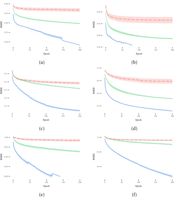
The discussion starts by analyzing the plots reported from Figure4.1(a) to Figure4.1(f).

Each plot displays the mean and standard error of the best training error (i.e., the fit-ness on known instances). Considering the training fitfit-ness, SLM shows the same evolution of fitness in all the considered datasets and it is the best performer among the other competitors. In some plots, like (a) and (f), the SLM produces fitness values that are not only better than the ones achieved by NEAT and SGA but it seems that fitness could improve further, if more epochs were considered. Furthermore, SGA outperforms NEAT on all displayed plots.

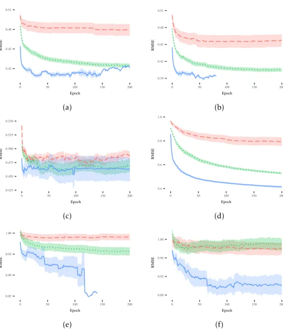
While results on the training set are important to understand the ability of the SLM to learn the model of the training data, it is even more important and interesting to evaluate its performance on unseen instances. Considering the plots reported from

Figure4.2(a) to Figure4.2(f), one can see that the SLM produces good quality solutions

that are able to generalize over unseen instances. In particular, the SLM presents a desirable behavior in the vast majority of problems, showing better or comparable per-formance with respect to the other competitors without overfitting the training data. Focusing on the other techniques, NEAT is the worst performer in 4 out of 6 datasets,

C H A P T E R 4 . E X P E R I M E N TA L S T U D Y 0.30 0.35 0.40 0.45 0.50 0 50 100 150 200 Epoch RMSE 0.36 0.40 0.44 0.48 0 50 100 150 200 Epoch RMSE (a) (b) 0.1 0.2 0.3 0.4 0.5 0 50 100 150 200 Epoch RMSE 0.4 0.6 0.8 1.0 0 50 100 150 200 Epoch RMSE (c) (d) 0.80 0.85 0.90 0.95 1.00 0 50 100 150 200 Epoch RMSE 0.6 0.8 1.0 0 50 100 150 200 Epoch RMSE (e) (f)

Figure 4.1: Evolution of mean and standard error of the best fitness on the training sets for the following datasets: (a) Credit; (b) Diabetes; (c) Sonar; (d) Concrete; (e)

Parkinson; (f) Music. The legend for all the plots is: NEAT SLM SGA

4 . 1 . R E S U LT S

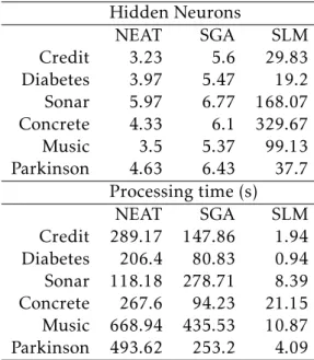
Table 4.1: Mean values for number of hidden neurons and processing time for NEAT, SGA and SLM on the Credit, Diabetes, Sonar, Concrete, Music and Parkinson dataset.

Hidden Neurons NEAT SGA SLM Credit 3.23 5.6 29.83 Diabetes 3.97 5.47 19.2 Sonar 5.97 6.77 168.07 Concrete 4.33 6.1 329.67 Music 3.5 5.37 99.13 Parkinson 4.63 6.43 37.7 Processing time (s) NEAT SGA SLM Credit 289.17 147.86 1.94 Diabetes 206.4 80.83 0.94 Sonar 118.18 278.71 8.39 Concrete 267.6 94.23 21.15 Music 668.94 435.53 10.87 Parkinson 493.62 253.2 4.09

while it achieves comparable performance with respect to the SGA in the remaining datasets. Also, plots (b) and (e) make apparent how SLM takes advantage of the EDV stopping criterion and terminates the evolutionary process before overfitting occurs. To summarize the results of this first part of the experimental phase, it is possible to state that the SLM is able to outperform SGA and NEAT with respect to the training fitness, by also producing models able to generalize over unseen instances. This is a very promising result that we are going to discuss more in the remaining part of the paper.

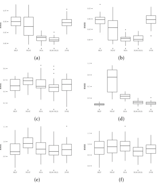
To that end, we reported in Figure4.3the results of SLM and other well-known

ma-chine learning techniques that are commonly used to solve classification and regression problems. Starting the discussion, it is possible to observe that the SLM tends to pro-duce competitive generalization errors in all the considered datasets. Regarding MLP and SVM, the SLM obtained better results for (a) and (b), while producing comparable solutions for the remaining problems. Comparing with SGA, SLM performs better on (a) and (d), with comparable results on the remaining datasets. Most importantly, SLM is able to outperform NEAT on all the displayed datasets. Finally, by analyzing

Table4.1, it is possible to compare the number of nodes of the models obtained with

the SLM , with NEAT, and SGA as well as the running time of these techniques. Al-though SLM produces the most complex (with the most hidden neurons) solutions, these solutions can be generated in a negligible amount of time. Compared to NEAT and SGA, SLM can develop solutions between one and two orders of magnitude faster (e.g. results on Credit).

All in all, at the end of the experimental campaign, it is possible to state that the SLM is a neuroevolution algorithm that is competitive with state of the art methods for

C H A P T E R 4 . E X P E R I M E N TA L S T U D Y 0.42 0.45 0.48 0.51 0 50 100 150 200 Epoch RMSE 0.39 0.42 0.45 0.48 0.51 0 50 100 150 200 Epoch RMSE (a) (b) 0.425 0.450 0.475 0.500 0.525 0.550 0 50 100 150 200 Epoch RMSE 0.4 0.6 0.8 1.0 0 50 100 150 200 Epoch RMSE (c) (d) 0.85 0.90 0.95 1.00 0 50 100 150 200 Epoch RMSE 0.88 0.92 0.96 1.00 0 50 100 150 200 Epoch RMSE (e) (f)

Figure 4.2: Evolution of mean and standard error of the best fitness on the testing sets for the following datasets: (a) Credit; (b) Diabetes; (c) Sonar; (d) Concrete; (e)

Parkinson; (f) Music. The legend for all the plots is: NEAT SLM SGA

4 . 1 . R E S U LT S ● ● 0.40 0.45 0.50 0.55

MLP NEAT SGA SLM (OLS) SVM

RMSE ● ● ●● 0.40 0.45 0.50 0.55

MLP NEAT SGA SLM (OLS) SVM

RMSE (a) (b) ● ● ● ● 0.3 0.4 0.5 0.6

MLP NEAT SGA SLM (OLS) SVM

RMSE ● 0.5 0.7 0.9 1.1

MLP NEAT SGA SLM (OLS) SVM

RMSE (c) (d) ● 0.9 1.0 1.1

MLP NEAT SGA SLM (OLS) SVM

RMSE ● 0.8 0.9 1.0 1.1

MLP NEAT SGA SLM (OLS) SVM

RMSE

(e) (f)

Figure 4.3: Boxplots of generalization error for the following datasets: (a) Credit; (b) Diabetes; (c) Sonar; (d) Concrete; (e) Parkinson; (f) Music. On each box, the central

mark is the median, the edges of the box are the 25th and 75th percentiles, and the

C H A P T E R 4 . E X P E R I M E N TA L S T U D Y

regression and classification problems and, built in a negligible amount of time and able to generalize over unseen instances. These features pave the way for future work in the area at the intersection between neuroevolution and deep learning, with the possibility of evolving the structure of deep networks in a tolerable amount of time.

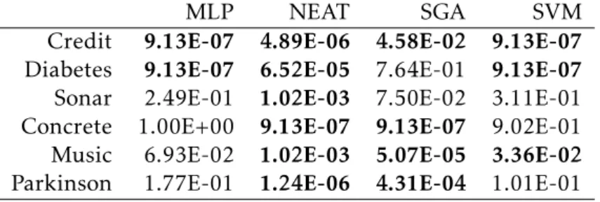
To assess the statistical significance of the results presented in Figure4.3, a statistical

validation was performed. The statistical validation considers, for each dataset, the SLM and compares it with the other techniques. First of all, given that is not possible to assume a normal distribution of the values obtained by running the different tech-niques, we ran the Shapiro-Wilk test and we considered a value of α = 0.05. The null hypothesis of this test is that the values are normally distributed. The result of the test suggests that the alternative hypothesis cannot be rejected. Hence, the Mann-Whitney U test with paired samples is conducted for comparing the results returned by the SLM and the other considered algorithms under the null hypothesis that the SLM’s median value is greater or equal to the competitive algorithm’s median value, across repeated measures. Also in this test a value of α = 0.05 was used and the Bonferroni correction

was considered. Table 4.2reports the p-values returned by the Mann-Whitney test,

and bold is used to denote values suggesting that the alternative hypotheses cannot be rejected. According to these results, out of 10 problems, the best SLM variant out-performs (1) MLP in 2 problems; (2) NEAT in 6 problems; (3) SGA in 4 problems; (4) SVM in 3 problems. On the Credit dataset, SLM can outperform all competitors with statistical significance. In the remaining comparisons, there was no evidence of statistically significant difference between the SLM and the other competitors.

Table 4.2: P-values for Mann-Whitney U test between SLM and competitive algorithms, where the null hypothesis states that the SLM’s median unseen error is greater or equal to the competitive algorithm’s median unseen error.

MLP NEAT SGA SVM

Credit 9.13E-07 4.89E-06 4.58E-02 9.13E-07

Diabetes 9.13E-07 6.52E-05 7.64E-01 9.13E-07

Sonar 2.49E-01 1.02E-03 7.50E-02 3.11E-01

Concrete 1.00E+00 9.13E-07 9.13E-07 9.02E-01

Music 6.93E-02 1.02E-03 5.07E-05 3.36E-02

Parkinson 1.77E-01 1.24E-06 4.31E-04 1.01E-01

4.2

Ensemble Approach

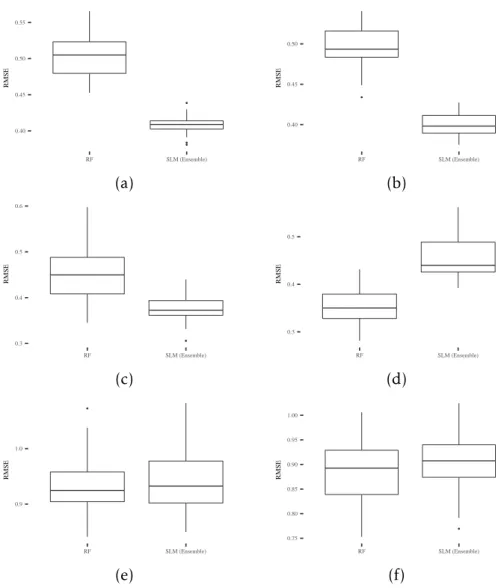
The promising results obtained at the end of the experimental phase, both in terms of performance, running time and number of neurons, led us to consider a new compari-son. In particular, we want to compare results achieved by considering an ensemble of SLM against the ones obtained with Random Forests (RFs) [3]. To perform this analysis, ensembles of 25 SLM models and tree predictors (for RFs) were built. The

4 . 2 . E N S E M B L E A P P R OAC H

comparison was performed considering the same datasets under study as introduced

in Section ??. Figure4.4reports the generalization error for the 6 considered datasets.

As one can see, the SLM ensemble outperforms the RFs ensemble on (a), (b) and (c), while generating comparable results in (e) and (f). These excellent results are also strengthened by the fact that the SLM ensemble model is formed by weak SLM learn-ers that contain only a few nodes (as already discussed in the previous analysis). To statistically validate the results of this comparison the same aforementioned statistical

procedure was used. The following p-values were obtained: 9.13e−07for (a), 9.13e−07

C H A P T E R 4 . E X P E R I M E N TA L S T U D Y ● ● ● 0.40 0.45 0.50 0.55 RF SLM (Ensemble) RMSE ● 0.40 0.45 0.50 RF SLM (Ensemble) RMSE (a) (b) ● 0.3 0.4 0.5 0.6 RF SLM (Ensemble) RMSE 0.3 0.4 0.5 RF SLM (Ensemble) RMSE (c) (d) ● 0.9 1.0 RF SLM (Ensemble) RMSE ● 0.75 0.80 0.85 0.90 0.95 1.00 RF SLM (Ensemble) RMSE (e) (f)

Figure 4.4: Boxplots of generalization error for the following datasets: (a) Credit; (b) Diabetes; (c) Sonar; (d) Concrete; (e) Parkinson; (f) Music. On each box, the central

mark is the median, the edges of the box are the 25th and 75th percentiles, and the

whiskers extend to the most extreme data points, excluding outliers.

C

h

a

p

t

e

r

5

C o n c lu s i o n

This paper studied different variants of the SLM algorithm, a recently proposed neu-roevolution method. Comparisons were performed against other neuneu-roevolution meth-ods and other well-established supervised machine learning methmeth-ods. It is shown that the best SLM variants are able to outperform most of remaining methods on the ma-jority of the 6 real-world datasets considered. Particularly interesting are the results of the SLM variation that computes the optimal mutation step for each application of the mutation operator, and that, at the same time, uses a recently proposed semantic stopping criterion to determine when to stop the search. This variant is able to evolve competitive neural networks in a few seconds on the vast majority of the datasets. An initial assessment of the usage of this SLM variant to create ensembles of neural network is also performed. This initial assessment shows that this approach is able to outperform the random forests algorithm on three out of six selected datasets.

B i b l i o g r a p h y

[1] T. Aaltonen, J Adelman, T Akimoto, M. Albrow, B. Á. González, S Amerio, D

Amidei, A Anastassov, A Annovi, J Antos, et al. “Measurement of the top-quark

mass with dilepton events selected using neuroevolution at CDF.” In:Physical

Review Letters 102.15 (2009), p. 152001.

[2] M. Bojarski, D. Del Testa, D. Dworakowski, B. Firner, B. Flepp, P. Goyal, L. D.

Jackel, M. Monfort, U. Muller, J. Zhang, et al. “End to end learning for

self-driving cars.” In:arXiv preprint arXiv:1604.07316 (2016).

[3] L. Breiman. “Random forests.” In:Machine learning 45.1 (2001), pp. 5–32.

[4] D. Ciregan, U. Meier, and J. Schmidhuber. “Multi-column deep neural networks

for image classification.” In: Computer vision and pattern recognition (CVPR),

2012 IEEE conference on. IEEE. 2012, pp. 3642–3649.

[5] P. Cortez and A. M. G. Silva. “Using data mining to predict secondary school

student performance.” In: (2008).

[6] I. Gonçalves, S. Silva, and C. M. Fonseca. “Semantic Learning Machine: A

Feedforward Neural Network Construction Algorithm Inspired by Geometric

Semantic Genetic Programming.” In:Progress in Artificial Intelligence. Vol. 9273.

Lecture Notes in Computer Science. Springer, 2015, pp. 280–285. i s b n: 978-3-319-23484-7.

[7] I. Gonçalves, S. Silva, C. M. Fonseca, and M. Castelli. “Unsure when to stop?

ask your semantic neighbors.” In: Proceedings of the Genetic and Evolutionary

Computation Conference. ACM. 2017, pp. 929–936.

[8] I. Gonçalves. “An Exploration of Generalization and Overfitting in Genetic

Programming: Standard and Geometric Semantic Approaches.” Doctoral disser-tation. Portugal: Department of Informatics Engineering, University of Coimbra, 2017.

[9] A. Krizhevsky, I. Sutskever, and G. E. Hinton. “Imagenet classification with deep

convolutional neural networks.” In: Advances in neural information processing

systems. 2012, pp. 1097–1105.

[10] M. Lichman. UCI Machine Learning Repository. 2013. u r l: http://archive.

B I B L I O G R A P H Y

[11] T. Mikolov, I. Sutskever, K. Chen, G. S. Corrado, and J. Dean. “Distributed

representations of words and phrases and their compositionality.” In:Advances

in neural information processing systems. 2013, pp. 3111–3119.

[12] A. Moraglio, K. Krawiec, and C. G. Johnson. “Geometric semantic genetic

pro-gramming.” In:International Conference on Parallel Problem Solving from Nature.

Springer. 2012, pp. 21–31.

[13] NEAT Python: Configuration file description.http://neat-python.readthedocs.

io/en/latest/config_file.html. Accessed: 2018-06-11.

[14] F. Pedregosa, G. Varoquaux, A. Gramfort, V. Michel, B. Thirion, O. Grisel, M.

Blondel, P. Prettenhofer, R. Weiss, V. Dubourg, J. Vanderplas, A. Passos, D. Cour-napeau, M. Brucher, M. Perrot, and E. Duchesnay. “Scikit-learn: Machine

Learn-ing in Python.” In: Journal of Machine Learning Research 12 (2011), pp. 2825–

2830.

[15] D. E. Rumelhart, G. E. Hinton, and R. J. Williams. “Learning representations by

back-propagating errors.” In:nature 323.6088 (1986), p. 533.

[16] B. E. Sakar, M. E. Isenkul, C. O. Sakar, A. Sertbas, F. Gurgen, S. Delil, H. Apaydin,

and O. Kursun. “Collection and analysis of a Parkinson speech dataset with

multiple types of sound recordings.” In: IEEE Journal of Biomedical and Health

Informatics 17.4 (2013), pp. 828–834.

[17] J. Secretan, N. Beato, D. B. D Ambrosio, A. Rodriguez, A. Campbell, and K. O.

Stanley. “Picbreeder: evolving pictures collaboratively online.” In:Proceedings

of the SIGCHI Conference on Human Factors in Computing Systems. ACM. 2008,

pp. 1759–1768.

[18] K. Simonyan and A. Zisserman. “Very deep convolutional networks for

large-scale image recognition.” In:arXiv preprint arXiv:1409.1556 (2014).

[19] K. O. Stanley and R. Miikkulainen. “Evolving neural networks through

aug-menting topologies.” In:Evolutionary computation 10.2 (2002), pp. 99–127.

[20] K. O. Stanley, B. D. Bryant, and R. Miikkulainen. “Real-time neuroevolution

in the NERO video game.” In:IEEE transactions on evolutionary computation 9.6

(2005), pp. 653–668.

[21] I. Sutskever, O. Vinyals, and Q. V. Le. “Sequence to sequence learning with

neural networks.” In: Advances in neural information processing systems. 2014,

pp. 3104–3112.

[22] P. A. Szerlip, A. K. Hoover, and K. O. Stanley. “Maestrogenesis:

Computer-assisted musical accompaniment generation.” In: (2012).

[23] F.-Y. Wang, J. J. Zhang, X. Zheng, X. Wang, Y. Yuan, X. Dai, J. Zhang, and L. Yang.

“Where does AlphaGo go: From church-turing thesis to AlphaGo thesis and

beyond.” In:IEEE/CAA Journal of Automatica Sinica 3.2 (2016), pp. 113–120.

B I B L I O G R A P H Y

[24] X. Yao. “A review of evolutionary artificial neural networks.” In: International

journal of intelligent systems 8.4 (1993), pp. 539–567.

[25] F. Zhou, Q Claire, and R. D. King. “Predicting the geographical origin of music.”

In: Data Mining (ICDM), 2014 IEEE International Conference on. IEEE. 2014,

A

p

p

e

n

d

i

x

A

Pa r a m e t e r C o n f i g u r a t i o n s

A P P E N D I X A . PA R A M E T E R C O N F I G U R AT I O N S

Table A.1: First set of NEAT parameter. Parameter names and values are taken from [13]. [] defines the beginning of a configuration section, {} defines a tunable

parameter from Section3.1.

Parameter Value fitness_criterion mean fitness_threshold 10 no_fitness_termination True pop_size {population_size} reset_on_extinction True [DefaultSpeciesSet] compatibility_threshold {compatibility_threshold} [DefaultStagnation] species_fitness_func mean max_stagnation 15 species_elitism 1 [DefaultReproduction] elitism 1 survival_threshold 0.2 min_species_size 1 [DefaultGenome] activation_default random activation_mutate_rate 0.01

activation_options sigmoid identity relu tanh

aggregation_default sum aggregation_mutate_rate 0 aggregation_options sum bias_init_mean 0 bias_init_stdev 1 bias_init_type gaussian bias_max_value 30 bias_min_value -30 bias_mutate_power 0.1 bias_mutate_rate 0.01 bias_replace_rate 0.01 compatibility_disjoint_coefficient {compatibility_disjoint_coefficient} compatibility_weight_coefficient {compatibility_weight_coefficient} 24

Table A.2: Second set of NEAT parameter. Parameter names and values are taken from [13]. [] defines the beginning of a configuration section, {} defines a tunable

parameter from Section3.1.

Parameter Value conn_add_prob {conn_add_prob} conn_delete_prob {conn_delete_prob} enabled_default True enabled_mutate_rate 0.01 enabled_rate_to_false_add 0 enabled_rate_to_true_add 0 feed_forward True initial_connection partial_nodirect 0.25 node_add_prob {node_add_prob} node_delete_prob {node_delete_prob} num_hidden 1 num_inputs {num_inputs} num_outputs 1 response_init_mean 1 response_init_stdev 0 response_init_type gaussian response_max_value 30 response_min_value -30 response_mutate_power 0 response_mutate_rate 0 response_replace_rate 0 single_structural_mutation False structural_mutation_surer True weight_init_mean 0 weight_init_stdev 1 weight_init_type gaussian weight_max_value 30 weight_min_value -30 weight_mutate_power {weight_mutate_power} weight_mutate_rate {weight_mutate_rate} weight_replace_rate 0.1

Table A.3: Parameter configuration search grid for Multilayer Perceptron. Parameter names according to [14]. Parameter Start (inclusive) End (inclusive) Step size (multiplicative) alpha 10−6 10−1 10 learning_rate_init 10−6 10−1 10 hidden_layer_sizes [(1), (2), (2, 2), (3, 3, 3), (5, 5, 5), (2, 2, 2, 2)]

A P P E N D I X A . PA R A M E T E R C O N F I G U R AT I O N S

Table A.4: Parameter configuration search grid for Support Vector Machine. Parameter names according to [14]. Parameter Start (inclusive) End (inclusive) Step size (additive) C 0.1 1 0.1 epsilon 0.1 0.5 0.1 degree 1 4 1 gamma 0.1 0.5 0.1 coef0 0.1 0.5 0.1

kernel [’linear’, ’poly’, ’rbf’, ’sigmoid’]

probability TRUE