Project Work presented as partial requirement for obtaining the Master’s degree in Information Management

(1)

i

Application of machine learning techniques for

solving real world business problems

Ineta Juozenaite

The case study

–

target marketing of insurance

policies

Project Work presented as partial requirement for obtaining

(2)

i

MEGI

2

017 Title: Application of machine learning techniques for solving real world business problems

Subtitle: The case study – target marketing of insurance policies

Student

(3)

(4)

ii

NOVA Information Management School

Instituto Superior de Estatística e Gestão de Informação

Universidade Nova de Lisboa

APPLICATION OF MACHINE LEARNING TECHNIQUES FOR SOLVING

REAL WORLD BUSINESS PROBLEMS. THE CASE STUDY

–

TARGET

MARKETING OF INSURANCE POLICIES

by

Ineta Juozenaite

Project Work presented as partial requirement for obtaining the Master’s degree in Information Management, with a specialization in Knowledge Management and Business Intelligence

Advisor:Mauro Castelli

(5)

iii

ACKNOWLEDGEMENTS

First of all, I would like to express my sincere gratitude to my advisor Professor Mauro Castelli for his support of my Master project work.

Also, I would like to thank a lot to my best friend and soulmate Gerda Gruzauskaite for her support, patience and motivation during this period.

(6)

iv

ABSTRACT

The concept of machine learning has been around for decades, but now it is becoming more and more popular not only in the business, but everywhere else as well. It is because of increased amount of data, cheaper data storage, more powerful and affordable computational processing. The complexity of business environment leads companies to use data-driven decision making to work more efficiently. The most common machine learning methods, like Logistic Regression, Decision Tree, Artificial Neural Network and Support Vector Machine, with their applications are reviewed in this work.

Insurance industry has one of the most competitive business environment and as a result, the use of machine learning techniques is growing in this industry. In this work, above mentioned machine learning methods are used to build predictive model for target marketing campaign of caravan insurance policies to achieve greater profitability. Information Gain and Chi-squared metrics, Regression Stepwise, R package “Boruta”, Spearman correlation analysis, distribution graphs by target variable, as well as basic statistics of all variables are used for feature selection. To solve this real-world business problem, the best final chosen predictive model is Multilayer Perceptron with backpropagation learning algorithm with 1 hidden layer and 12 hidden neurons.

KEYWORDS

(7)

v

INDEX

1. Introduction ... 1

2. Study Objectives ... 3

3. Machine Learning Methods ... 4

3.1. Logistic Regression ... 4

3.1.1. Overview of the Method ... 4

3.1.2. Applications of Logistic Regression ... 4

3.2. Decision Tree ... 4

3.2.1. Overview of the Method ... 4

3.2.2. Applications of Decision Trees ... 5

3.3. Artificial Neural Networks ... 6

3.3.1. Overview of the Method ... 6

3.3.2. Applications of Artificial Neural Networks ... 7

3.4. Support Vector Machines ... 9

3.4.1. Overview of the Method ... 9

3.4.2. Applications of Support Vector Machines ... 10

4. Evaluation Techniques ... 11

5. Predictive Modelling for Direct Marketing In Insurance Sector ... 13

5.1. Data Source ... 13

5.2. Data Exploration and Pre-processing ... 13

5.3. Variable Selection ... 18

5.3.1. Information Gain and Chi-squared ... 18

5.3.2. Stepwise Logistic Regression ... 19

5.3.3. R Package “Boruta”

... 19

5.3.4. Variables Combinations ... 20

5.4. Data Partitioning... 21

5.5. Building Predictive Model ... 22

5.5.1. Choosing the Final Variables Combination ... 22

5.5.2. Final Predictive Model ... 23

5.5.3. The Graphs of the Final Model ... 25

5.6. Predictions

–

Scoring Unseen Data ... 26

6. Conclusion ... 27

7. Bibliography ... 28

(8)

vi

8.1. Variables List ... 32

8.2. Basic Analysis by Each Level of Each Predictor Variable ... 36

8.3. Histograms by Target Variable ... 54

8.4. Spearman Correlation Between Predictor Variables and Target Variable... 68

8.5. Spearman Correlation Between Independent Variables ... 69

8.6. Predictive Models Results with Various Variables Combinations ... 81

8.7. Models Results with Different Seeds ... 88

(9)

vii

LIST OF FIGURES

Figure 3.1

–

Decision Tree structure ... 5

Figure 3.2

–

Neural Network structure ... 7

Figure 3.3

–

Visual explanation of Support Vector Machine ... 9

Figure 5.1

–

Number of caravan insurance holders ... 14

Figure 5.2 - Histograms of age, contribution to car policies and number of car policies

variables by dependent variable ... 15

Figure 5.3 - Graphical presentation of Spearman correlation matrix ... 17

Figure 5.4

–

Information Gain and Chi-squared bar charts... 18

Figure 5.5

–

Feature selection by “Boruta” algorithm

... 20

Figure 5.6

–

Weighted sum square error graph of the final model ... 25

(10)

viii

LIST OF TABLES

Table 4.1

–

Confusion Matrix ... 11

Table 5.1

–

Training and Test datasets ... 22

Table 5.2

–

Results of each variables subset ... 23

Table 5.3

–

The results obtained from 10 different partitioned datasets ... 24

Table 5.4

–

The final predictive model performance ... 26

Table 8.1

–

Variables List ... 34

Table 8.2- Description of variables values ... 36

Table 8.3

–

Analysis of the independent variables ... 53

Table 8.4

–

Spearman correlations between independent variables and dependent variable

... 69

Table 8.5

–

Subsections of Spearman’s correlation matrix of all independent variables.

... 70

Table 8.6

–

1st subsection of the Spearman correlation matrix ... 71

Table 8.7

–

2nd subsection of the Spearman correlation matrix... 72

Table 8.8

–

3rd subsection of the Spearman correlation matrix ... 73

Table 8.9

–

4th subsection of the Spearman correlation matrix ... 74

Table 8.10

–

5th subsection of the Spearman correlation matrix ... 75

Table 8.11

–

6th subsection of the Spearman correlation matrix ... 76

Table 8.12

–

7th subsection of the Spearman correlation matrix ... 77

Table 8.13

–

8th subsection of the Spearman correlation matrix ... 78

Table 8.14

–

9th subsection of the Spearman correlation matrix ... 79

Table 8.15

–

10th subsection of the Spearman correlation matrix ... 80

Table 8.16

–

Predictive models results with various variables combinations ... 88

(11)

ix

LIST OF ABBREVIATIONS AND ACRONYMS

ANN Artificial Neural Network

CART Classification and Regression Tree

CHAID Chi-square Automatic Interaction Detector

DT Decision Tree

LR Logistic Regression

ML Machine Learning

MLP Multilayer Perceptron

PCA Principal Component Analysis

RBF Radial Basis Function Kernel

SVM Support Vector Machine

(12)

1

1. INTRODUCTION

Machine learning techniques can be defined as automated systems that are able to extract useful information from data or to make predictions based on existing, already collected data (Mohri, Rostamizadeh & Talwalkar, 2012). In 1959, one of machine learning pioneers, Arthur Samuel defined machine learning as “the field of study that gives computers (or machine) that ability to learn without being explicitly programmed” (Samuel, 1959). It means that machine learning algorithms can iteratively learn from data without being programmed to perform specific tasks. Machine learning models are able to adapt independently when new data are presented into the model. These models learn from prior computations to present reliable results and to make right decisions based on the produced results. ("Machine Learning: What it is and why it matters", 2017; Mathivanan & Rajesh, 2016)

Analytics thought leader Thomas H. Davenport (2013) states the importance of machine learning in organizations: “Humans can typically create one or two good models a week, machine learning can create thousands of models a week”. Machine learning goal is to give an increasing level of automation in getting knowledge and taking certain decisions by replacing human activity with automatic systems that can be more accurate and would save huge amount of human time than doing the same things by themselves (Mohri, Rostamizadeh, & Talwalkar, 2012).

(13)

2 these improvements and research, that proved the benefits, have increased the potential of machine learning – and the need for business.

Machine learning techniques are used in variety of industries, education, medicine, chemistry, and a lot of other science fields. Machine learning approaches are applied to solve real-world business problems, like found in financial services, transportation, or in marketing and sales perspectives. For the banks and other financial businesses, machine learning is used to identify investment opportunities, clients with high-risk profiles, when to trade or prevent fraud. In transportation industry, like in delivery companies or public transportation, machine learning approaches are applied to find inherent patterns and trends for making routes more efficient and for predicting potential problems on the road. In the marketing and sales perspectives, machine learning methods are used for customer churn prediction, target marketing or it is also used to analyse buying behaviour of customers and make promotions based on analysis. (Linoff & Berry, 2011; "Machine Learning: What it is and why it matters", 2017)

The example of financial services can be insurance industry that has one of the most competitive business environment and because of this, the use of machine learning techniques is growing in this industry (Ansari & Riasi, 2016). Some of the most common examples, where machine learning can be used in insurance companies, are fraud detection, underwriting, claims processing and customer services, including marketing and sales of insurance policies. (Ansari & Riasi, 2016; Delgado-Gómez, Aguado, Lopez-Castroman, Santacruz & Artés-Rodriguez, 2011; Jost, 2016; Salcedo-Sanz, Fernández-Villacañas, Segovia-Vargas & Bousoño-Calzón, 2005; Umamaheswari & Janakiraman, 2014).

(14)

3

2. STUDY OBJECTIVES

The main objective of this work is to solve a real-world business problem by using machine learning approaches. In this work case, the desirable outcome is to build a model that would be able to predict if customers are interested in purchasing insurance policy or not, based on data about customers like usage product data and sociodemographic data. To build a predictive model for binary classification problem few different machine learning approaches are used. According to the performance results of the models, the best one is chosen for target marketing campaign.

To achieve the main objective, the following objectives are identified.

▪ To describe the chosen machine learning approaches that will be used in this

work.

▪ To describe and prepare data for the chosen techniques.

▪ To apply chosen machine learning techniques, combine them, and try to

improve the predictive model.

(15)

4

3. MACHINE LEARNING METHODS

This section presents 4 of the most popular machine learning techniques for solving the real-world business problems. This section reveals specific business problems and approaches that are used to solve each of the problems. Logistic Regression (LR), Decision Tree (DT), Artificial Neural Network (ANN), Support Vector Machine (SVM) are well established, reliable and efficient methods. These 4 machine learning methods have been chosen to solve a real-world business problem of this work. Based on the literature review, these methods show great popularity and good performance in solving difficult business problems that are similar to the main problem of this work. Another reason of choosing above mentioned methods is their implementation in R, that is the software used in the predictive model building.

3.1. L

OGISTIC

R

EGRESSION

3.1.1. Overview of the Method

Logistic regression is a method of predictive analysis and it is used to solve classification problems. In logistic regression, the aim is to find a model that fits the regression curve, y = f(x), the best. Here y is dependent categorical variable, while x represents independent variables that can be continuous, categorical or both at the same time. (Shalev-Shwartz & Ben-David, 2014)

3.1.2. Applications of Logistic Regression

Logistic regression is a popular and easily understandable classification technique that is often used for building prediction models to solve various business problems. For example, it can be used for customer churn prediction (Gürsoy, 2010; Neslin, Gupta, Kamakura, Lu & Mason, 2006; Vafeiadis, Diamantaras, Sarigiannidis & Chatzisavvas, 2015), customer segmentation (McCarty & Hastak, 2007) as well as direct marketing (Coussement, Harrigan & Benoit, 2015; Zahavi & Levin, 1997). Gürsoy (2010) in his work shows that after proper data transformation, logistic regression can achieve good results. However, in most of the reviewed literature it did not perform well comparing to more advanced machine learning techniques (Coussement, Harrigan & Benoit, 2015; Delgado-Gómez, Aguado, Lopez-Castroman, Santacruz & Artés-Rodriguez, 2011; Neslin, Gupta, Kamakura, Lu & Mason, 2006; McCarty & Hastak, 2007; Vafeiadis, Diamantaras, Sarigiannidis & Chatzisavvas, 2015). Sometimes real-world business problems can be too complex for logistic regression to solve it. Also, more advanced machine learning techniques are able to improve the performance by learning from data (Mitchell, 1997) and this makes statistical techniques like logistic regression to be less effective. For this reason, there is need to introduce more advanced and complex machine learning techniques.

3.2. D

ECISION

T

REE

3.2.1. Overview of the Method

(16)

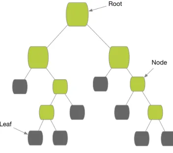
5 The Figure 3.1 illustrates the structure of decision tree that is similar to the structure of the tree. DT method splits the dataset into homogenous sub-sets according to the best splitter of input variables. The splitting process stops when defined stopping criterion is reached. In the case when there is no stopping criterion, dataset is classified perfectly in the complete grown tree. The examples of the stopping criteria can be constraints of the tree size like defining the minimum number of observations in the nodes or maximum depth of the tree. Constraints of the tree size help to avoid over-fitting but this is the greedy approach. Another method to avoid over-fitting is tree pruning with two different techniques: pre-pruning and post-pruning. Pre-pruning stops splitting the tree before the dataset is classified perfectly. Post-pruning removes sub-nodes of perfectly classified dataset that do not bring high classification power. (Breiman, Friedman, Olshen & Stone, 1984; Shalev-Shwartz & Ben-David, 2014)

Figure 3.1 – Decision Tree structure

To split dataset and choose the best splitter, decision trees use various algorithms. One of them is CART (Classification and Regression Tree) algorithm that is suitable to use for binary classification problem, the same problem as there is in the empirical studies of this work. CART is designed to use for both classification and regression problems. This algorithm builds binary trees and uses Gini index in order to determine the best next split. CART algorithm uses post-pruning techniques to avoid over-fitting. In this empirical work, the cost-complexity pruning technique is used together with CART algorithm. (Breiman, Friedman, Olshen & Stone, 1984; Rokach & Maimon, 2014)

3.2.2. Applications of Decision Trees

(17)

6 This method can be used in customer segmentation (McCarty & Hastak, 2007). Decision trees are helpful to understand what characteristics customer has in each group, making easy the process of assigning a new customer to a specific group (McCarty & Hastak, 2007). Moreover, Goonetilleke and Caldera (2013), as well as Soeini and Rodpysh (2012) use decision trees for insurance customer attrition. To reduce the rate of attrition is substantial issue in insurance companies. Also, it can be used in prediction of salesman performance as it was done in the work by Delgado-Gómez, Aguado, Lopez-Castroman, Santacruz and Artés-Rodriguez (2011). Another example where decision trees can be applied is target marketing, defining if a customer belongs to the responder or the non-responder group. Coussement, Harrigan and Benoit (2015) in their work use 3 different decision tree algorithms (CHAID, CART, C4.5) to build customer response model for direct mail marketing. Comparing with all used methods in their work, CHAID and CART are in the group of methods that has the best performance, while C4.5 algorithm has quite poor performance. Furthermore, decision trees can be used for customer churn prediction. In the work that was done by Vafeiadis, Diamantaras, Sarigiannidis and Chatzisavvas (2015), decision tree C5.0 algorithm, that is persisted version of C4.5 algorithm, is applied to solve a problem of customer churning by using telecommunication data. As it was written above, C4.5 algorithm has not shown a good performance to solve direct mail targeting problem (Coussement, Harrigan & Benoit, 2015), while its followed-up version C5.0, that is used to solve customer churning problem (Vafeiadis, Diamantaras, Sarigiannidis & Chatzisavvas, 2015), is one of the most effective method among other used techniques, excluding boosted machine learning techniques.

However, decision trees performance depends on the structure of the data. Decision trees algorithms have tendency to perform poorly if there are many complex and non-linear relationships between attributes (Vafeiadis, Diamantaras, Sarigiannidis & Chatzisavvas, 2015). For this reason, the methods that can deal better with complex relationships between attributes are reviewed.

3.3. A

RTIFICIAL

N

EURAL

N

ETWORKS

3.3.1. Overview of the Method

Artificial neural network is computational model based on structure of very simplified human brain model. Like in human brains, neural network uses large number of computational units, also called neurons. Neurons are connected to each other, and also are able to communicate with each other in a complex network where complicated calculations are able to perform. (Shalev-Shwartz & Ben-David, 2014)

(18)

7 Figure 3.2 – Neural Network structure

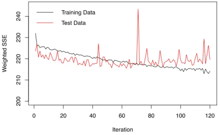
In this work, Multilayer Perceptron (MLP) is chosen with backpropagation learning algorithm. One hidden layer is used, and the number of hidden neurons is changed from 1 to 20. The activation function of input and hidden layer is logistic function, as well as for the output layer since our work problem is binary classification. The initial weights of neural network are assigned randomly, and because of the existence of local optimum, MLP converges to the different results each time it is run. It explains some of the peaks in the training and test errors graphs. To be able to produce the same model again, it is important to remember to initialize random generator with the specific seed before building the model. All chosen specifications are based on the research of literature review that was done in this work.

Multilayer Perceptron is a feedforward model with the same structure as a single layer Perceptron, but with addition of one or more hidden layers. Backpropagation is mostly used learning algorithm for multilayer neural networks. Multilayer Perceptron with backpropagation algorithm has two steps: forward and backward. The first step is forward, where outputs are calculated propagating the inputs through activation function from input layer to output layer. In this step, the weights of all connections remain the same. In the second backward step, the weight of each connection is modified. For the output neurons, the weights are changed using Delta Rule, and for the hidden neurons the weights are changed by propagating backward the error of the output neurons to the hidden neurons. The error of the hidden neuron is calculated by summing the errors of all output neurons to which it is connected directly. (Shalev-Shwartz & Ben-David, 2014)

3.3.2. Applications of Artificial Neural Networks

(19)

8 also has significant influence on ANN functioning and it makes ANN powerful machine learning approach (Miikkulainen, 2011; Tkáč & Verner, 2016).

One example of the complex problems for which ANN can be used is churn prediction. To build classifier for insurance policy holders who are about to terminate their policy, Goonetilleke and Caldera (2013) use neural network with Multilayer Perceptron structure and backpropagation learning algorithm, that performs better than another used machine learning method – Decision Tree C4.5. In addition, Vafeiadis, Diamantaras, Sarigiannidis and Chatzisavvas (2015) in their work use ANN approaches to build model for customer churning in telecommunication industry. These authors train Multilayer Perceptron model using backpropagation with one hidden layer and a varying number of hidden neurons. ANN with 15 hidden units shows the best performance going side by side with another machine learning method - Decision Tree 5.0 (Vafeiadis, Diamantaras, Sarigiannidis & Chatzisavvas, 2015). However, corresponding to reviewed articles (Mozer, Wolniewicz, Grimes, Johnson & Kaushansky, 2000; Vafeiadis, Diamantaras, Sarigiannidis & Chatzisavvas, 2015; Wai-Ho Au, Chan & Xin Yao, 2003) for customer churn prediction problem ANNs have better performance than logistic regression and decision trees.

Another example of ANNs in insurance companies is presented by Rahman, Arefin, Masud, Sultana and Rahman (2017). They use neural network with Multilayer Perceptron structure and backpropagation learning algorithm to predict the behaviour of future insurance policy owners by classifying them as regular or irregular premium payers. Insurance company, that is able to identify regular future payers, increases its profit significantly (Rahman, Arefin, Masud, Sultana & Rahman, 2017).

Furthermore, Coussement, Harrigan, and Benoit (2015) use ANNs for direct marketing to build response model and this is another complex business problem where ANN can be applied. In their work (Coussement, Harrigan & Benoit, 2015), Multilayer Perceptron model with one hidden layer is one of the best performing machine learning approaches but at the same time competing with decision trees CHAID and CART. For both described problems ANN with one hidden layer is chosen, even though as many hidden layers as necessary can be used in building ANN model. Most of the problems can be solved using one or two layers, even though the problem is quite complex, one-two hidden layers are powerful enough to approximate any function (Bishop, 1995; Coussement, Harrigan & Benoit, 2015).

(20)

9 and Lizana (2016), where artificial neural network outperforms support vector machine and gives the best results. As a result of this, it is still necessary to review support vector machine methods and to see their applications.

3.4. S

UPPORT

V

ECTOR

M

ACHINES

3.4.1. Overview of the Method

Support Vector Machine (SVM) is more refined and more recent method of machine learning. As it was written before, this method achieves a global optimum in the training phase and it is the advantage of SVM against ANN (Julio, Giesen & Lizana, 2016). However, it does not mean that SVM will give the better results than ANN (Julio, Giesen & Lizana, 2016).

Support vector machine can be used for both classification and regression problems. The main specification of SVM is the usage of Kernel function, and another one is that local optimum does not become global optimum in SVM algorithms (Shalev-Shwartz & Ben-David, 2014). In empirical studies of this work, SVM, that is suitable for classification problem, is used and described below.

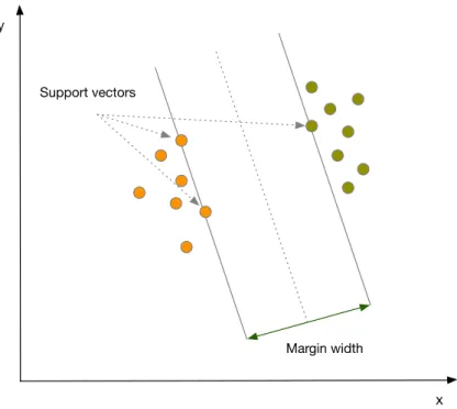
To separate two classes SVM finds the optimal hyperplane between them by maximizing the margin between closest points of classes, that are also called support vectors. The optimal hyperplane is the line in the middle of the margin (Shalev-Shwartz & Ben-David, 2014). The Figure 3.3 provides the visual explanation of SVM. Having hyperplane that separates data records into non-overlapping classes can cause over-fitting. To avoid this, SVM finds the optimal hyperplane not only by maximizing the margin, but also by minimizing the misclassification. (Shalev-Shwartz & Ben-David, 2014)

(21)

10 For difficult real-world business problems data is not linearly separable. SVM manages this by projecting data points into other dimensional space, usually higher, where the same data points would be linearly separable. To map data in different space, SVM uses non-linear functions. In this work, Kernel Gaussian Radial Basis (Kernel RBF) function is chosen based on the literature review, and because it is general function for classification problems with a good performance. Another good factor, there are only two parameters that must be defined, C and. C is the cost of misclassification. For SVM a high value of parameter C lets to misclassify as less training cases as possible and in this way prediction function becomes complex, while for the low value of parameter C is opposite. Parameter  defines which training examples are considered as support vectors by the model. If value of the parameter is high, only the closest training examples, and vice versa for low value . (Karatzoglou, Meyer & Hornik, 2006; Shalev-Shwartz & Ben-David, 2014)

3.4.2. Applications of Support Vector Machines

(22)

11

4. EVALUATION TECHNIQUES

To evaluate models and to select the one with the best performance, evaluation techniques of models like accuracy and F-measure are used in empirical studies of this work. Both measures are calculated based on confusion matrix (see the Table 4.1), which shows all true positive (TP), false negative (FN), false positive (FP) and true negative (TN) values of classifier. (Vafeiadis, Diamantaras, Sarigiannidis & Chatzisavvas, 2015)

Predicted: NO Predicted: YES

Actual: NO True Negative

(TN)

False Positive (FP)

Actual: YES False Negative

(FN)

True Positive (TP) Table 4.1 – Confusion Matrix

In the above table, the confusion matrix for binary classifications (no and yes) is presented. True Positives (TP) identify the cases where events (yes cases) are classified correctly, while True Negatives (TN) - correctly predicted non-events (no cases). False Positives (FP) show wrongly classified events, it means the events are predicted as no cases, but actually they are yes cases. False Negatives (FN) show wrongly identified non-events (no cases), more clearly, no cases are identified as yes cases.

Accuracy is the proportion of the total number of predictions that were correct. The formula:

F-measure is a combination of sensitivity and positive predictive value, that also can be called precision. The formula:

The sensitivity measures the proportion of actual positives that are correctly identified. The formula:

The precision is the proportion of positives that were correctly identified. The formula:

(23)

(24)

13

5. PREDICTIVE MODELLING FOR DIRECT MARKETING IN INSURANCE SECTOR

All data analysis and model building is done with R programming language. R is a free software that compiles on a different UNIX platforms and systems. R has a wide range of various statistical and graphical techniques, and it is able to be extended to the other much difficult level like creating your own functions or procedures ("R: The R Project for Statistical Computing", n.d.). The R code of this work data analysis can be found in Appendix 8.8.

5.1. D

ATA

S

OURCE

The data source that is used in this work for empirical studies was provided by the Dutch data mining company Sentient Machine Research and is based on a real-world business problem (“Sentient Machine Research”, 2000). This data source contains information about customers of insurance company, and also the results of already performed marketing campaign “Caravan Insurance Policy” that tells if customers were interested in this insurance policy or not.

Dataset to train and test predictive models consists of 5822 customers. The customers are described by 86 variables, including sociodemographic data and product ownership data. Also, including target variable that gives information if customer purchased caravan insurance policy or not. The sociodemographic data is obtained from customers’ zip codes. It means that customers with the same zip code are characterized with the same sociodemographic features. The validation dataset, that helps to build better predictive model, is not used because of the small size of sample (Maimon & Rokach, 2005). Dataset for predictions consist of 4000 customers with the same attributes excluding target variable which is supposed to be returned by chosen model.

In the Appendix 8.1, there are two tables with all variables and their explanations.

5.2. D

ATA

E

XPLORATION AND

P

RE

-

PROCESSING

Before applying techniques that are going to be used for the empirical studies, data has to be explored and pre-processed. It means that data should be analysed in order to get familiar with it and also to recognise possible data pre-processing techniques. Pre-processing techniques are cleaning techniques that detect and remove errors and inconsistencies from data, like outliers that could cause misinterpretation of analysis (Han, Kamber, & Pei, 2012).

(25)

14 Figure 5.1 – Number of caravan insurance holders

The above Figure 5.1 shows distribution of target variable - caravan policy owners. It reveals that the data is very imbalanced. Only 6% of customers purchased caravan policy. It is not surprising that data is imbalanced because usually solving direct marketing problems there are more non-responders than responders (Ling & Li, 1998; Pan & Tang, 2014).

(26)

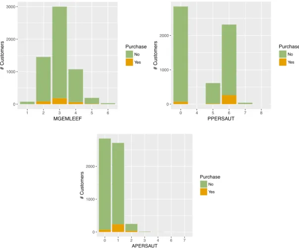
15 To present information visually, the histograms of each variable by dependent variable are created as well. The histograms of all variables can be found in the Appendix 8.3. However, since the percentage of customers with caravan insurance policy is very low, it is hard to see from the histograms which variables give clearly visible distribution between purchasing insurance policy and which ones not. Having a quick look to histograms, it has not escaped the notice that there are not many customers in the 20 - 30 age range, while customers in the 40 - 50 age group tend to purchase caravan insurance policy. Also, the histogram of variable PPERSAUT shows that customers who spent averagely 1000 – 4999 money for car policies have a tendency to hold a caravan insurance policy. In addition, customers who have one car insurance policy are more likely to get caravan insurance policy (variable APERSAUT). The histograms of these 3 variables are shown in the Figure 5.2.

Figure 5.2 - Histograms of age, contribution to car policies and number of car policies variables by dependent variable

In exploration phase, Spearman correlation analysis between variables has been performed. Spearman correlation method is appropriate to use when the variables are not normally distributed or the relationship between the variables is not linear. These reasons determine to use Spearman rank correlation method.

(27)

16 variables with target variable are the contribution of third party insurance firms (PWABEDR) and the purchased number of the same insurance (AWABEDR). The correlation is less than 0,001.

Also, the Spearman correlation matrix between all independent variables has been calculated and can be found in the Appendix 8.5. Since there are 85 variables, the Spearman correlation matrix of independent variables is visualized in the Figure 5.3 to have a quick view in it, too. In this correlation matrix plot, it is easy to see which variables are highly correlated and which ones not. In this graphical presentation of Spearman correlation matrix, the intensity of correlation is presented by the colour and the ellipse form. The stronger the correlation, the more narrowed ellipse. If the ellipse is shown from the left to the right, the correlation is positive, and vice versa. Also, the colour identifies the sign of the correlation. The blue shows positive and the red – negative. It is useful to look at correlation matrix for variables transformations, because the highly correlated variables might be beneficial to merge into one variable. Sometimes data source might contain similar variables that give the same information, so before eliminating any variable it is good to see correlations between them. Having highly correlated variables in the predictive model might make the predictive model unstable.

There are 4 variables about marital status: MRELGE (Married), MRELSA (Living together), MRELOV

(Other relation), MFALLEN (Singles). These variables are quite correlated among each other, so it has been decided to leave only one variable that shows the percentage of single people in the customer’s neighbourhood. In this way, the percentage of single or not single people is clear. MFGEKIND

(Household without children) and MFWEKIND (Household with children) variables show the same information, how many households there are with children and without, and also these variables are quite correlated. Household with children variable has higher correlation with target variable, so it has not been removed from the variable set. Also, dataset contains two variables MHHUUR (rented house) and MHKOOP (home owners) that present the same information and have a high correlation between each other (0,999), so MHKOOP variable has been eliminated from the dataset. There is the same situation with the variables MZFONDS (national health service) and MZPART (private health insurance), that also have a correlation close to 1 between each other, so only one variable is left,

MZFONDS. Moreover, there are 3 variables that shows information about the number of having cars. Since these variables are also quite correlated and MAUT2 does not have a high correlation with target variable, it is enough to know if there is at least one car or not, so it is decided to leave only one variable MAUT0 to have that information.

Furthermore, there are several groups of variables in which any highly correlated variables have not been detected so that it would be possible to eliminate some of them. One of that groups of variables shows the customer’s status (high status, entrepreneur, farmer, middle management, skilled labours, unskilled labours), the second group of variables presents social class (social class A, B1, B2, C, D), and the third one shows the average income. In addition, it is worth to mention that the dataset contains some kind of similar variables with a high correlation between each other that have not been eliminated. At this stage, it is still not clear which variables having in the variables combination would bring a higher value to the predictive model. The example of these variables could be the main type of customer and the subtype of customer.

(28)

17 policies, are very highly correlated. For example, the variable that shows contribution of car policies and the variable that shows the number of car policies have correlation equal to 1, other correlations of these variables combinations are also very close to 1. This reason motivated to create another variable, that would include these two types of variables. The most reasonable combination of these two types of variables is multiplication that would show the interaction of the variables. So, the primary product ownership variables have been eliminated and the new combinations of these variables are going to be used in the predictive model. Since all variables contain grouped values, it is hard to think about more variables transformations that would make sense for the predictive modelling.

To sum up, after eliminating and creating new variables, the final dataset contains 46 variables, from which 31 variables presents sociodemographic data, 14 variables presents product ownership data and also the target variable is included in the final dataset.

(29)

18

5.3. V

ARIABLE

S

ELECTION

Based on variable selection techniques and also already gained knowledge from data exploration phase, the variables subsets are created, so that they could be tested to detect which of them brings the highest value to the predictive model.

5.3.1. Information Gain and Chi-squared

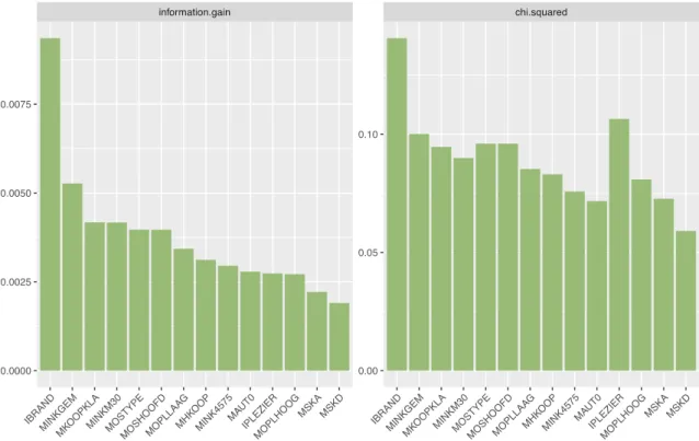
First of all, Information Gain and Chi-squared metrics are calculated to see the feature importance for each variable. The Figure 5.4 illustrates these metrics in the bar charts. The graphs show only 14 variables because for other variables the metrics are equal to zero. As it was clarified earlier in this work, these graphs also display that there is any variable that would explain well caravan insurance policy owners. These graphs give the idea of importance of each separate variable to prediction. However, building the prediction model the combination of the variables, that gives a high value to predictive model, is necessary. On the other hand, these metrics reveal the variables that does not have any worth to prediction and the variables that might be eliminated from further analysis. As it can be seen from Information Gain and Chi-squared bar charts, the transformed variable (IBRAND) from the number of fire policies and contribution to fire policies has the highest importance to prediction. Based on Information Gain, the second variable with the highest importance is the average income (MINKGEM) while looking to Chi-squared metric it is the interaction variable of boat policies. Both of these variables look more meaningful than the first one – the fire policies variable. It is quite hard to explain why the fire policies has the highest impact to prediction, but it is essential to emphasize that the worth to prediction of each variable is very low.

(30)

19

5.3.2. Stepwise Logistic Regression

The second method, that is used for variable selection, is stepwise logistic regression. This method selects the model by AIC criterion using forward stepwise regression, backward stepwise regression or combination of both, subtraction and addition of variables to the model. The lowest AIC value gives the model with the best variables combination.

This method showed that the best variable combination is from 17 variables: MGEMLEEF (Average age), MOPLMIDD (Medium level education), MOPLLAAG (Lower level education), MBERBOER

(Farmer), MBERMIDD (Middle management), MSKC (Social class C), MHKOOP (home owners),

MAUT0 (No car), MINK123M (Income >123.000), MINKGEM (Average income), IWERKT (Interaction of agricultural machines policies), IBROM (Interaction of moped policies), IWAOREG (Interaction of disability insurance policies), IBRAND (Interaction of fire policies), IPLEZIER (Interaction of boat policies), IFIETS (Interaction of bicycle policies), IBYSTAND (Interaction of social security insurance policies).

5.3.3. R P

ackage “Boruta”

The third method to select variables is used from R package “Boruta”. This variable selection algorithm is based on Random Forest. It eliminates variables that do not perform well recursively at each iteration. At the end, Boruta algorithm presents all variables, either they are relevant to the model or not, by showing if the variable has been rejected or not. So, Boruta shows even the variables that give small relevance to the prediction. ("Wrapper Algorithm for All Relevant Feature Selection [R package Boruta version 5.2.0]", 2017)

(31)

20 Figure 5.5 – Feature selection by “Boruta” algorithm

5.3.4. Variables Combinations

Based on the results obtained from above described methods, also gained insights from Spearman correlation analysis and distribution graphs, 7 variables subsets have been created to test on all machine learning models in order to choose the best variables subset:

Variables sets:

1. All sociodemographic variables that have not been eliminated in exploring

variables stage as well as all transformed product ownership variables:

MOSTYPE, MAANTHUI, MGEMOMV, MGEMLEEF, MOSHOOFD, MFALLEEN,

MFWEKIND, MOPLHOOG, MOPLMIDD, MOPLLAAG, MBERHOOG, MBERZELF,

MBERBOER, MBERMIDD, MBERARBG, MBERARBO, MSKA, MSKB1, MSKB2,

MSKC, MSKD, MHKOOP, MAUT0, MZPART, MINKM30, MINK3045, MINK4575,

MINK7512, MINK123M, MINKGEM, MKOOPKLA, IAANHANG, ITRACTOR,

IWERKT, IBROM, ILEVEN, IPERSONG, IGEZONG, IWAOREG, IBRAND, IZEILPL,

IPLEZIER, IFIETS, IINBOED, IBYSTAND

. Total of 46 variables.

2. Variables, that did not have zero importance to prediction, obtained from

(32)

21

MINKM30, MOSTYPE, MOSHOOFD, MOPLLAAG, MHKOOP, MINK4575, MAUT0,

IPLEZIER, MOPLHOOG, MSKA, MSKD

. Total of 14 variables.

3. Variables selected from stepwise regression method:

MGEMLEEF, MOPLMIDD,

MOPLLAAG, MBERBOER, MBERMIDD, MSKC, MHKOOP, MAUT0, MINK123M,

MINKGEM, IWERKT, IBROM, IWAOREG, IBRAND, IPLEZIER, IFIETS, IBYSTAND

.

Total of 17 variables.

4. Variables that have been confirmed by Boruta algorithm from R package:

IPLEZIER, MOSTYPE, MOPLLAAG, MOPLHOOG, MSKA, MOSHOOFD, MFALLEEN,

MSKC, IBRAND, MBERARBO, MOPLMIDD, MINKM30, MBERARBG, MZPART,

MINKGEM,

MKOOPKLA,

MAUT0,

MINK7512,

MFWEKIND,

MHKOOP,

MBERMIDD, MBERHOOG, MBERBOER, MSKD, MGEMLEEF, MINK4575, MSKB1,

MINK3045, MBERZELF, MGEMOMV, MSKB2, ITRACTOR, IBROM, IBYSTAND

.

Total of 34 variables.

5. The total variables mixture based on all performed variable selection methods:

IPLEZIER, MOSTYPE, MOPLLAAG, IBRAND, MBERARBO, MZPART, MINKGEM,

MKOOPKLA, MAUT0, MHKOOP, MBERMIDD, MGEMLEEF, ITRACTOR, IBROM,

IBYSTAND, MINK123M, IZEILPL

. Total of 17 variables.

6. Variables mixture that includes all transformed product ownership variables

and mixture of sociodemographic variables, that have been selected based on

all performed variable selection methods:

MOSTYPE, MOPLLAAG, MBERARBO,

MZPART, MINKGEM, MKOOPKLA, MAUT0, MHKOOP, MBERMIDD, MGEMLEEF,

MINK123M, IPLEZIER, IBRAND, ITRACTOR, IBROM, IBYSTAND, IWAOREG,

IGEZONG, IFIETS, IAANHANG, IINBOED, ILEVEN, IWERKT, IPERSONG, IZEILPL

.

Total of 25 variables.

7. Variables mixture that has been built by testing various combinations of the

variables. It includes all transformed product ownership variables, and also

mixture of variables that showed the highest importance to prediction in

variable selection methods:

MKOOPKLA, MINKGEM, MOPLLAAG, MHKOOP,

MAUT0, IPLEZIER, IBRAND, ITRACTOR, IBROM, IBYSTAND, IWAOREG, IGEZONG,

IFIETS, IAANHANG, IINBOED, ILEVEN, IWERKT, IPERSONG, IZEILPL

. Total of 19

variables.

5.4. D

ATA

P

ARTITIONING

(33)

22 the model built by using training dataset. The third test dataset is used to estimate the accuracy of the model on unseen data that gives realistic performance of the model. (Reitermanov, 2010)

Following practical recommendations, in this work data is going to be divided into 2 datasets – 70% training and 30% test. There is not going to be the validation dataset because of the small size of the sample. (Maimon & Rokach, 2005)

The chosen partition method is stratified sampling. The method explores the structure of the dataset and divides it into homogenous sets. Stratified sampling assures that all three datasets, training, validation and test, are well balanced (Reitermanov, 2010). Usually solving direct marketing problems, the data is imbalanced because there are more non-responders than responders. This is the main reason why stratified method is chosen. (Ling & Li, 1998; Pan & Tang, 2014)

5.5. B

UILDING

P

REDICTIVE

M

ODEL

Before starting to build model, the number of customers that will be selected in the test and predictive datasets should be defined. The boundary probability that would help to select potential customers should be defined. The customers with a higher probability of purchasing caravan insurance policy than the boundary probability would be selected. The boundary probability depends on the costs of contacting potential caravan insurance customers and the profit of selling insurance policies. Without knowing it, it has been decided to select 20% of the customers with the highest probability to purchase the caravan insurance policy.

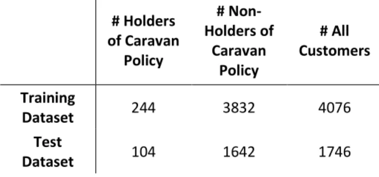
After splitting dataset to training and test datasets, the test dataset has 1746 customers with 104 caravan insurance policy owners. The numbers of customers of each dataset are displayed in the Figure 5.1.

# Holders of Caravan

Policy

# Non-Holders of

Caravan Policy

# All Customers

Training

Dataset 244 3832 4076

Test

Dataset 104 1642 1746

Table 5.1 – Training and Test datasets

By selecting 20% customers of the test dataset, 349 customers with the highest probability of having insurance policy are going to be selected to test all models. Selecting 349 customers randomly from the test dataset, approximately 21 caravan insurance policy holders should appear there. This number is going to be as the base line for the obtained results from the predictive models. If the model gives the number of correctly identified policy holders close to this number, it means the model performance is really poor and more analysis should be done to get better results.

5.5.1. Choosing the Final Variables Combination

(34)

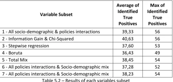
23 used for predictive modelling. In the Appendix 8.6, there is a table with the evaluation metrics (Identified True Positives, Sensitivity, Precision and F-measure), that are described in the 4th_section,

for all possible combinations of chosen variables subsets and machine learning techniques. The Table 5.2 presents the average of identified true positives of all used models for each variables subset, and also the maximum of identified true positives. In this table, it is encouraging to see that for all variables subsets the average of identified true positives is higher than random guess. Also, keeping in mind that some of the used machine learning methods did not perform very well decreased the average. The detailed table is in the Appendix 8.6.

Variable Subset

Average of Identified

True Positives

Max of Identified

1 - All socio-demographic & policies interactions 39,33 56

2 - Information Gain & Chi-Squared 40,63 56

3 - Stepwise regression 37,60 53

4 - Boruta 36,43 49

5 - Total Mix 38,45 54

6 - All policies interactions & Socio-demographic mix 37,28 52 7 - All policies interactions & Socio-demographic mix 38,23 54

Table 5.2 – Results of each variables subset

The variables subset that has been created based on Information Gain and Chi-squared metrics has the highest average of correctly identified caravan policy holders. The variables subset of all not removed variables has very similar results, as well as the fifth and the seventh variables subsets. In the first and the second variables subsets there are quite many variables that are highly correlated with each other and it might make the predictive model unstable. While the fifth subset contains also some highly correlated variables but less than in the seventh subset, and also considering that the seventh subset has less variables than the fifth, it is decided to choose the seventh variables subset as the final variables combination for predictive model building.

5.5.2. Final Predictive Model

The final chosen variables that are included in the predictive model are the variables from the seventh variables subset. It includes all transformed product ownership variables (IPLEZIER, IBRAND, ITRACTOR, IBROM, IBYSTAND, IWAOREG, IGEZONG, IFIETS, IAANHANG, IINBOED, ILEVEN, IWERKT, IPERSONG, IZEILPL) and also mixture of variables that showed the highest importance to prediction in variable selection methods (MKOOPKLA – Purchasing power class, MINKGEM – Average income,

MOPLLAAG – Lower level education, MHKOOP – Home owners, MAUT0 – No car). The highest number of correctly identified caravan policy holders with these variables is 54. It is higher than the number 21, that would be obtained by selecting customers randomly.

(35)

24 datasets helps to choose the final model as well as to test how much models are stable. The detailed results of all 10 different partitioned datasets are presented in the Appendix 8.7.

To choose the best model, the average of correctly identified caravan insurance owners and the highest number of identified true positives are calculated for each model (see the Table 5.3).

Model

Average of Identified

Model

Average of Identified

Logistic Regression 43,6 48 MLP - 19 neurons 42,2 50

CART 42,6 50 MLP - 20 neurons 42,1 52

MLP - 1 neuron 28,4 49 SVM gamma = 0.001 C = 10 26,8 34

MLP - 2 neurons 42 47 SVM gamma = 0.001 C = 20 28,9 41

MLP - 3 neurons 43,5 50 SVM gamma = 0.001 C = 30 28,2 36 MLP - 4 neurons 43,4 48 SVM gamma = 0.001 C = 40 26,5 33 MLP - 5 neurons 43,1 50 SVM gamma = 0.001 C = 50 28,3 35 MLP - 6 neurons 43,2 51 SVM gamma = 0.001 C =

100 29,3 38

MLP - 8 neurons 41,7 49 SVM gamma = 0.01 C = 20 28,7 36 MLP - 9 neurons 42,1 49 SVM gamma = 0.01 C = 30 27,7 40 MLP - 10 neurons 42,8 50 SVM gamma = 0.01 C = 40 28,5 40 MLP - 11 neurons 43,2 52 SVM gamma = 0.01 C = 50 24,3 33

MLP - 14 neurons 41,9 53 SVM gamma = 0.1 C = 20 26,8 37

MLP - 18 neurons 42,8 54 SVM gamma = 0.1 C = 100 27,5 40 Table 5.3 – The results obtained from 10 different partitioned datasets

Based on the produced results of the Table 5.3, Multilayer Perceptron with 12 hidden neurons is chosen as the best model. This model has the highest correctly identified caravan insurance holders in average, and also with this model the highest number of correctly identified customers is obtained. As well as Sensitivity, Precision and F-measure of this model are the highest compared to other models (see in the Appendix 8.7).

(36)

25

5.5.3. The Graphs of the Final Model

Figure 5.6 – Weighted sum square error graph of the final model

(37)

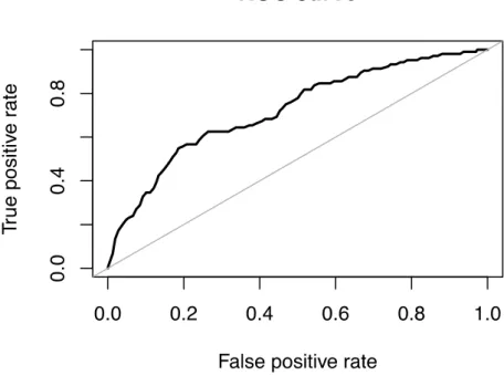
26 Figure 5.7 – ROC curve of the final model

The figure 5.7 displays ROC curve of the final model. ROC curve shows the relationship between true positive rate and false positive rate for all possible cut-offs. The closer curve is to the diagonal, the lower accuracy of the model is.

5.6. P

REDICTIONS

–

S

CORING

U

NSEEN

D

ATA

From prediction dataset, with the final predictive model 800 potential customers, that have the highest possibility to purchase caravan insurance policy, are identified. Having targets for prediction dataset, that are provided by the company Sentient Machine Research, it is possible to know that 104 potential caravan insurance holders have been identified correctly by the final chosen predictive model. The prediction dataset has 238 caravan insurance holders, so the obtained result is quite good. Randomly selecting customers from prediction dataset, it is possible to identify around 48 caravan insurance holders, so the performance of selected predictive model gives more than 50% better results. For more detailed results, see the Table 5.4.

Model Seed

True Positives in

the Test dataset

Identified True Positives

Random

Guess Lift Sensitivity Precision F-measure

MLP - 12

neurons 888 238 104 48 56 0,437 0,130 0,200

(38)

27

6. CONCLUSION

Using the data about insurance customers from the company Sentient Machine Research, data analysis has been made and useful information has been extracted. This allowed to identify the customers with the highest probability to purchase insurance caravan policy in order to contact them for direct marketing campaign of caravan insurance policies.

The main aim of the project is achieved, the predictive model to solve a real-world business problem is built. The final model correctly predicted 104 customers from 800 selected customers from prediction dataset. It is a half more correctly identified potential customers than it would have been achieved by random selection. The accuracy of the final model is not high but it is important to emphasize that dataset contains only 6% caravan insurance policy holders. This made some difficulties in variable selection and model building phases.

From 86 variables none of them with the significant importance to the prediction has been found. Any variable is not able to separate clearly enough caravan insurance holders and non-holders. The subset of the variables that would be important for prediction had to be found. In this work phase, Information Gain and Chi-squared metrics, Regression Stepwise, R package “Boruta”, Spearman correlation analysis, distribution graphs by target variable, as well as basic statistics of all variables are used to select variables combinations. For the future works, it is recommended to do better analysis for possible techniques to select variables for predictive model. One of them could be Principal Component Analysis (PCA). Also, it is advisable to do more variable transformations, for example, variable that represents the sub-type of customer could be split to binary variables.

Moreover, it should be remarked that sociodemographic data presents information not about exact customer but about the area in which customer is living in. To increase the accuracy of the predictive model it would be useful to have this information by each customer. However, to gain this data is quite difficult for insurance company because of the customers’ privacy.

(39)

28

7. BIBLIOGRAPHY

Author, A. A., Author, B. B., & Author, C. C. (Year). Title of article. Title of Periodical, volume number

(issue number), pages.

Ansari, A., & Riasi, A. (2016). Modelling and evaluating customer loyalty using neural networks: Evidence from startup insurance companies. Future Business Journal, 2(1), 15-30.

Benoit, D., & Van den Poel, D. (2012). Improving customer retention in financial services using kinship network information. Expert Systems With Applications, 39(13), 11435-11442.

Bishop, C. (1995). Neural networks for pattern recognition. Oxford: Oxford University Press.

Bohanec, M., Kljajić Borštnar, M., & Robnik-Šikonja, M. (2017). Explaining machine learning models in sales predictions. Expert Systems With Applications, 71, 416-428.

Breiman, L., Friedman, J. H., Olshen, R. A., & Stone, C. J. (1984). Classification and regression trees.

Wadsworth & Brooks. Monterey, CA.

Brynjolfsson, E., Hitt, L., & Kim, H. (2011). Strength in Numbers: How Does Data-Driven Decisionmaking Affect Firm Performance?. SSRN Electronic Journal.

Carbonell, J., Michalski, R., & Mitchell, T. (1983). Machine learning. Pittsburgh, Pa.: Dept. of Computer Science, Carnegie-Mellon University.

Coussement, K., Harrigan, P., & Benoit, D. (2015). Improving direct mail targeting through customer response modeling. Expert Systems With Applications, 42(22), 8403-8412.

Davenport, T. (2013). Industrial-Strength Analytics with Machine Learning. WSJ. Retrieved 13 June 2017, from https://blogs.wsj.com/cio/2013/09/11/industrial-strength-analytics-with-machine-learning/?mod=wsj_streaming_latest-headlines

Delgado-Gómez, D., Aguado, D., Lopez-Castroman, J., Santacruz, C., & Artés-Rodriguez, A. (2011). Improving sale performance prediction using support vector machines. Expert Systems With Applications, 38(5), 5129-5132.

du Jardin, P. (2017). Dynamics of firm financial evolution and bankruptcy prediction. Expert Systems With Applications, 75, 25-43.

Galar, M., Fernandez, A., Barrenechea, E., Bustince, H., & Herrera, F. (2012). A Review on Ensembles for the Class Imbalance Problem: Bagging-, Boosting-, and Hybrid-Based Approaches. IEEE Transactions On Systems, Man, And Cybernetics, Part C (Applications And Reviews), 42(4), 463-484.

Goonetilleke, T. O., & Caldera, H. A. (2013). Mining life insurance data for customer attrition analysis.

Journal of Industrial and Intelligent Information, 1(1).

(40)

29 Han, J., Kamber, M., & Pei, J. (2012). Data mining. Amsterdam: Elsevier/Morgan Kaufmann.

Jordan, M., & Mitchell, T. (2015). Machine learning: Trends, perspectives, and prospects. Science,

349(6245), 255-260.

Jost, P. (2016). Competitive insurance pricing with complete information, loss-averse utility and finitely many policies. Insurance: Mathematics And Economics, 66, 11-21.

Julio, N., Giesen, R., & Lizana, P. (2016). Real-time prediction of bus travel speeds using traffic shockwaves and machine learning algorithms. Research In Transportation Economics, 59, 250-257.

Karatzoglou, A., Meyer, D., & Hornik, K. (2006). Support Vector Machines in R. Journal Of Statistical Software, 15(9), 1-28.

Kerdprasop, N., Kongchai, P., & Kerdprasop, K. (2013). Constraint mining in business intelligence: A case study of customer churn prediction. International Journal of Multimedia and Ubiquitous Engineering, 8(3), 11-20.

Kim, Y., & Street, W. (2004). An intelligent system for customer targeting: a data mining approach.

Decision Support Systems, 37(2), 215-228.

Ling, C. X., & Li, C. (1998). Data mining for direct marketing: Problems and solutions. KDD, 98, 73-79. Linoff, G. S., & Berry, M. J. (2011). Data mining techniques: for marketing, sales, and customer

relationship management. John Wiley & Sons.

Machine Learning: What it is and why it matters. (2017). Sas.com. Retrieved 12 June 2017, from https://www.sas.com/en_us/insights/analytics/machine-learning.html

Maimon, O., & Rokach, L. (2005). Data mining and knowledge discovery handbook. New York: Springer.

Mathivanan, B., & Rajesh, R. (2016). Communication and Power Engineering. Walter de Gruyter GmbH & Co KG.

McCarty, J., & Hastak, M. (2007). Segmentation approaches in data-mining: A comparison of RFM, CHAID, and logistic regression. Journal Of Business Research, 60(6), 656-662.

Miikkulainen, R. (2011). Topology of a Neural Network. In Encyclopedia of Machine Learning. Springer US.

Mitchell, T. (1997). Machine Learning. New York: McGraw-Hill.

Mohri, M., Rostamizadeh, A., & Talwalkar, A. (2012). Foundations of machine learning. Cambridge, MA: The MIT Press.

(41)

30 Mozer, M., Wolniewicz, R., Grimes, D., Johnson, E., & Kaushansky, H. (2000). Predicting subscriber

dissatisfaction and improving retention in the wireless telecommunications industry. IEEE Transactions On Neural Networks, 11(3), 690-696.

Neslin, S., Gupta, S., Kamakura, W., Lu, J., & Mason, C. (2006). Defection Detection: Measuring and Understanding the Predictive Accuracy of Customer Churn Models. Journal Of Marketing Research, 43(2), 204-211.

Pan, Y., & Tang, Z. (2014). Ensemble methods in bank direct marketing. Service Systems and Service Management (ICSSSM), 1-5.

Parloff, R. (2016). Why Deep Learning Is Suddenly Changing Your Life. Fortune. Retrieved 13 June 2017, from http://fortune.com/ai-artificial-intelligence-deep-machine-learning/

Perlich, C., Dalessandro, B., Raeder, T., Stitelman, O., & Provost, F. (2013). Machine learning for targeted display advertising: transfer learning in action. Machine Learning, 95(1), 103-127. Pyle, D., & Jose, C. (2015). An executive’s guide to machine learning. McKinsey & Company. Retrieved

13 June 2017, from http://www.mckinsey.com/industries/high-tech/our-insights/an-executives-guide-to-machine-learning

Rahman, M. S., Arefin, K. Z., Masud, S., Sultana, S., & Rahman, R. M. (2017). Analyzing Life Insurance Data with Different Classification Techniques for Customers’ Behavior Analysis. In Advanced Topics in Intelligent Information and Database Systems (15-25). Springer International Publishing.

Reitermanov, Z. (2010). Data splitting. WDS, 10, 31-36.

Rokach, L., & Maimon, O. (2014). Data mining with decision trees: theory and applications. World scientific.

Salcedo-Sanz, S., Fernández-Villacañas, J., Segovia-Vargas, M., & Bousoño-Calzón, C. (2005). Genetic programming for the prediction of insolvency in non-life insurance companies. Computers & Operations Research, 32(4), 749-765.

Samuel, A. (1959). Some Studies in Machine Learning Using the Game of Checkers. IBM Journal Of Research And Development, 3(3), 210-229.

Sentient Machine Research. (2000). The Insurance Company (TIC), Amsterdam, Amsterdam: Author. Shalev-Shwartz, S., & Ben-David, S. (2014). Understanding machine learning. New York: Cambrige

University Press.

Soeini, R. A., & Rodpysh, K. V. (2012). Applying data mining to insurance customer churn management. Int. Proc. Comput. Sci. Inf. Technol, 30, 82-92.

(42)

31 Umamaheswari, K., & Janakiraman, S. (2014). Role of Data mining in Insurance Industry. An

international journal of advanced computer technology, 3(6), 961-966.

Vafeiadis, T., Diamantaras, K., Sarigiannidis, G., & Chatzisavvas, K. (2015). A comparison of machine learning techniques for customer churn prediction. Simulation Modelling Practice And Theory,

55, 1-9.

Wai-Ho Au, Chan, K., & Xin Yao. (2003). A novel evolutionary data mining algorithm with applications to churn prediction. IEEE Transactions On Evolutionary Computation, 7(6), 532-545.

Wrapper Algorithm for All Relevant Feature Selection [R package Boruta version 5.2.0]. (2017).

Cran.r-project.org. Retrieved 26 September 2017, from https://cran.r-project.org/web/packages/Boruta/index.html

Zahavi, J., & Levin, N. (1997). Applying neural computing to target marketing. Journal of Interactive Marketing, 11(4), 76-93.

Zhang, C., & Ma, Y. (2012). Ensemble Machine Learning. Dordrecht: Springer.

(43)

32

8. APPENDIX

8.1. V

ARIABLES

L

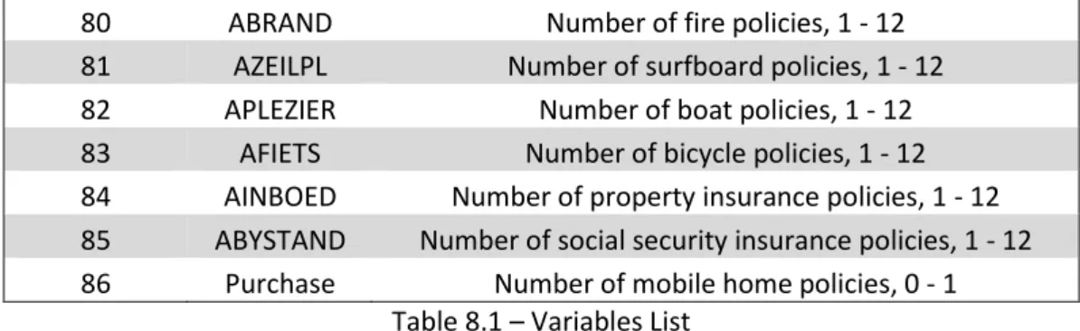
IST

In the below table, there are presented all variables with the variable number in the data source, name, description and containing values and their meaning.

Number Name Description

1 MOSTYPE Customer Subtype, see L0

2 MAANTHUI Number of houses, 1-10

3 MGEMOMV Average size household, 1 – 6

4 MGEMLEEF Average age, see L1

5 MOSHOOFD Customer main type, see L2

6 MGODRK Roman catholic, see L3

7 MGODPR Protestant, see L3

8 MGODOV Other religion, see L3

9 MGODGE No religion, see L3

10 MRELGE Married, see L3

11 MRELSA Living together, see L3