Characterizing phytoplankton biomass seasonal cycles in two NE Atlantic coastal bays

(1)

Continental Shelf Research 207 (2020) 104200

Available online 6 August 2020

(http://creativecommons.org/licenses/by-nc-nd/4.0/).

Characterizing phytoplankton biomass seasonal cycles in two NE Atlantic

coastal bays

Mariana Santos

a,b,*

_{, Helena Mouri˜no}

c,d

_{, Maria Teresa Moita}

a,e

_{, Alexandra Silva}

a

_,

Ana Amorim

b,c

_{, Paulo B. Oliveira}

a

a_{IPMA, I.P. – Instituto Portuguˆes do Mar e da Atmosfera, Rua Alfredo Magalh˜aes Ramalho, 6, 1495-006, Lisbon, Portugal}

b_{MARE - Centro de Ciências do Mar e do Ambiente, Faculdade de Ciências, Universidade de Lisboa, Campo Grande, 1749-016, Lisbon, Portugal} c_{Departamento de Biologia Vegetal, Faculdade de Ciências, Universidade de Lisboa, Campo Grande, 1749-016, Lisbon, Portugal}

d_{CMAF-CIO - Centro de Matemática, Aplicações Fundamentais e Investigação Operacional, Faculdade de Ciências, Universidade de Lisboa, Campo Grande, 1749-016,} Lisbon, Portugal

e_{CCMAR – Centro de Ciˆencias do Mar, Universidade do Algarve, Campus de Gambelas, 8005-139, Faro, Portugal}

A R T I C L E I N F O Keywords: Chlorophyll a seasonality Time series In situ data Ocean color Iberian upwelling coast

A B S T R A C T

The seasonal and interannual variability of chlorophyll a was studied between 2008 and 2016 in two coastal bays located in the northeastern limit of the Iberia/Canary upwelling ecosystem. The work aims (i) to understand if small latitudinal distances and/or coastline orientation can promote different chlorophyll a seasonal cycles; and (ii) to investigate if different meteorological and oceanographic variables can explain the differences observed on seasonal cycles. Results indicate three main biological seasons with different patterns in the two studied bays. A uni-modal pattern with a short early summer maximum and relatively low chlorophyll a concentration char-acterized the westernmost sector of the South coast, while a uni-modal pattern charchar-acterized by high biomass over a long period, slightly higher in spring than in summer, and high chlorophyll a concentration characterized the central West coast. Comparisons made between satellite estimates of chlorophyll a and in situ data in one of the bays revealed some important differences, namely the overestimation of concentrations and the anticipation of the beginning and end time of the productive period by satellite. Cross-correlation analyses were performed for phytoplankton biomass and different meteorological and oceanographic variables (SST, PAR, UI, MLD and precipitation) using different time lags to identify the drivers that promote the growth and the high levels of phytoplankton biomass. PAR contributed to the increase of phytoplankton biomass observed during winter/mid- spring, while upwelling and SST were the main explanatory drivers to the high Chl-a concentrations observed in late-spring/summer. Zonal transport was the variable that contributed most to the phytoplankton biomass during late-spring/summer in Lisbon Bay, while the meridional transport combined with SST was more important in Lagos Bay.

1. Introduction

Chlorophyll a concentration is usually used as a proxy for phyto-plankton biomass in aquatic ecosystems. The assessment of interannual variability of phytoplankton biomass requires the use of long time series, ideally spanning several decades. Long time series of in situ data are rare due to their high dependence on funding cycles and human resources. As a pigment, chlorophyll a can be estimated using satellite ocean color sensors. Since 1978, when the first satellite sensor to monitor ocean color (CZCS- Coastal Zone Color Scanner) was launched by NASA

(National Aeronautics and Space Administration), satellite imagery has been used to routinely measure chlorophyll a variability in the ocean. Since then, sensors with better spectral resolution, improved calibration and new algorithms have been developed (IOCCG, 2000). The high spatial-temporal coverage of chlorophyll a provided by satellite obser-vations revolutionized the understanding of the role of phytoplankton on global primary production (e.g. Field et al., 1998; Taboada et al., 2019; Tilstone et al., 2009). However, although remote sensing of ocean color is “relatively-simple” on waters where the optical properties can be described as a function of phytoplankton concentration (Case 1 waters),

* Corresponding author. MARE - Faculdade de Ciˆencias, Universidade de Lisboa, Campo Grande, 1749-016, Lisbon, Portugal.

E-mail addresses: msvsantos@fc.ul.pt, msvsantos@fc.ul.pt (M. Santos), mhnunes@fc.ul.pt (H. Mouri˜no), tmoitagarnel@gmail.com (M.T. Moita), amsilva@ipma.pt (A. Silva), aaferreira@fc.ul.pt (A. Amorim), pboliveira@ipma.pt (P.B. Oliveira).

Contents lists available at ScienceDirect

Continental Shelf Research

journal homepage: http://www.elsevier.com/locate/csr

https://doi.org/10.1016/j.csr.2020.104200

(2)

it has significant limitations in optically complex coastal areas where the optical properties do not depend only on chlorophyll concentration (Case 2 waters). In Case 2 waters there is a significant contribution of other particulate matter and/or yellow substances to the optical prop-erties (IOCCG, 2000). This increases the need for a wider grid of in situ observations to validate the data obtained by remote sensing (IOCCG, 2000).

Several studies have highlighted the influence of specific environ-mental drivers to phytoplankton variability in space and time. Effects on phytoplankton growth have been associated with variables such as the mixing and stratification of the water column, euphotic zone depth, wind forcing, coastal upwelling, surface irradiance and levels of nutrient concentrations (e.g. Behrenfeld and Boss, 2018; Krug et al., 2017, 2018;

Navarro et al., 2012). The analysis of chlorophyll a time series and correlated environmental variables can lead to the discrimination of the relative importance of phytoplankton variability drivers (Cloern et al., 2016). This is especially challenging in dynamic environments such as upwelling ecosystems (Lamont et al., 2014). An effective management of coastal ecosystems requires a multidisciplinary perspective to under-stand how processes operate together in biological changes (Cloern et al., 2016), and must take into account the spatial and temporal variability of the different phytoplankton drivers (Tweddle et al., 2018). In fact, there is a need to clearly understand the underlying mechanisms related to changes in phytoplankton biomass, phenological patterns, primary production and community composition (Cloern et al., 2016).

In coastal upwelling regions, coastal topography and coastline ir-regularities such as capes and bays produce variations in coastal wind, alongshore currents, chemistry and biology (Chavez and Messi´e, 2009;

Largier, 2020). On wind-exposed capes, strong upwelling and horizontal advection occur, while on the lee side of such promontories the winds, upwelling and horizontal advection are weaker (Chavez and Messi´e, 2009). Strong gradients are generated between the new upwelled waters off a cape and the protected shadow waters (Chavez and Messi´e, 2009). As a result, high levels of phytoplankton biomass are sustained in these ‘‘upwelling shadows” (e.g., Graham and Largier, 1997; Largier, 2020;

Oliveira et al., 2009a), which makes these regions more susceptible to the occurrence of harmful algal blooms (HABs) (Kudela et al., 2005;

Moita et al., 2003; Ryan et al., 2014). These features were observed in several upwelling regions, suggesting that these “upwelling shadows” may be characteristic features of these regions and play a significant role in the local biology (Graham and Largier, 1997 and references therein;

Largier, 2020). Although frequent and of high importance, these shallow coastal embayments are still poorly studied (Walter et al., 2018).

The Portuguese continental coast, located on the western Iberian Peninsula, is in the northeastern limit of the Iberia/Canary upwelling ecosystem, associated with the North Atlantic anticyclonic gyre (Wooster et al., 1976). This region is characterized by several prominent topographic features, such as capes, promontories and submarine can-yons (Relvas et al., 2007). It is also a complex area characterized by different mesoscale structures that are observed at a seasonal timescale, like fronts, jets, upwelling filaments and countercurrents (Haynes et al., 1993; Peliz et al., 2002; Relvas and Barton, 2005). In Portugal, up-welling occurs between spring and early autumn due to seasonally prevailing northerly winds, being stronger in summer (Fiúza et al., 1982;

Goela et al., 2016; Relvas and Barton, 2002; Wooster et al., 1976). During autumn and winter, while some episodes of upwelling may occur, there is a prevalence of downwelling inducing southerly winds (Alvarez et al., 2008; Goela et al., 2016).

Here we investigated for the North Atlantic Iberian upwelling system the relevance of small latitudinal distances and/or coastline orientation on chlorophyll a seasonal cycles, and the meteorological and oceano-graphic variables that may explain the observed temporal and spatial variability. To reach these goals, the present study focused on 9 years (2008–2016) of chlorophyll a data from two coastal bays, Lisbon and Lagos Bays, located in the upwelling shadow of two prominent Iberian headlands, Cape Roca and Cape S˜ao Vicente, respectively. For one of the

bays (Lisbon Bay), satellite estimates were compared with in situ data to assess the ability of L4 ocean color products to reproduce the near-coast chlorophyll a seasonal cycles.

2. Material and methods

2.1. Study area

This work was conducted in two geographically distinct coastal bays located on the West and South Portuguese continental coast, Lisbon and Lagos Bays, respectively (Fig. 1). Lisbon Bay (LisB) is located SE of Cape Roca (CR) under the strong influence of seasonal upwelling and of the Tagus river flow. Between spring and early autumn, under steady northerly winds, upwelling occurs and a recurrent upwelling filament rooted at CR extends southward or westward of the bay (Moita et al., 2003; Oliveira et al., 2009a). Due to the coastline discontinuity, this bay was considered by previous studies an upwelling shadow area where phytoplankton can be accumulated through different retention mecha-nisms (Moita et al., 2003; Oliveira et al., 2009b). The Tagus river, with a mean annual flow of 10 km3 ₍_{SNIRH, 2017}_{), is the main source of}

freshwater into the bay (Valente and da Silva, 2009) and is an important source of nutrients, with higher concentrations recorded during winter and early-spring (Cabrita et al., 2015). The conjunction of riverine and upwelling inputs sustains the availability of nutrients all year round in this region (Ferreira et al., 2019). The sampling site, referred to as LisB-IS, is a long-term monitoring station located about 12 km from CR (Fig. 1) at the entrance of a recreational marina in the north side of the bay (38◦41’36.82′′N, 9◦24′52.93′′W).

Lagos Bay (LagB) is at the SW limit of Iberia and is located to the east of Cape S˜ao Vicente (CSV) (Fig. 1). CSV is a coastline discontinuity that separates the West coast from the South coast. This Cape is a major upwelling center when north winds are predominant (Goela et al., 2016;

Relvas and Barton, 2002), spreading the cold upwelled water along the southern coast’s shelf break and slope (Relvas et al., 2007). On the South coast, during summer, a westward warm coastal countercurrent from the Gulf of C´adiz is recurrently observed which under favorable condi-tions can turn northward around CSV (Relvas and Barton, 2002, 2005;

Relvas et al., 2007). Although occasional, upwelling events also occur in the South coast under westerly winds (Goela et al., 2016; Relvas and Barton, 2002), occasionally leading to the reversal of the above-mentioned summer alongshore flow (Relvas and Barton, 2002). Upwelling is the main source of nutrients in the region of CSV (Cravo et al., 2010). To the east of LagB is the Arade river, with a much lower mean annual flow, 0.05 km3_{, than the Tagus river (}_{SNIRH, 2017}_).

2.2. In situ chlorophyll a biomass

In situ chlorophyll a (Chl-a) data were gathered only in LisB. Weekly

water samples were collected from 2008 to 2016 at the coastal station referred to as LisB-IS. The samples were collected under the National Monitoring Program of Harmful Algal Bloom species (HABs) led by IPMA, I.P. - Instituto Portuguˆes do Mar e da Atmosfera (National Insti-tute for the Sea and Atmosphere). Integrated water samples (0–7 m depth) were collected with a hose, always 1 h before high tide, to reduce the influence of the Tagus river and to optimize the direct influence of coastal waters on this nearshore station.

Water samples were stored in dark thermal bottles, for about half an hour, and analyzed in triplicate (250 mL each) in the laboratory. Each triplicate was vacuum filtered through 0.45 μm nitrate cellulose

mem-branes. Pigments were extracted with 90% acetone and Chl-a was determined according to the “Turner Fluorometer” method ( Holm--Hansen et al., 1965) on a Fluorescence Spectrophotometer (Hitachi F-7000).

(3)

Continental Shelf Research 207 (2020) 104200

2.3. Ocean color, meteorological, oceanographic and hydrographic data

Ocean color (OC) satellite data were extracted for the study period (2008–2016) for LisB, referred to as LisB-Sat, and for LagB, referred to as LagB-Sat (Fig. 1). Data were gathered from the reprocessed “Global Ocean” L4 satellite products available on CMEMS (Copernicus Marine Environment Monitoring Service, http://marine.copernicus.eu/), namely the datasets:

oc-glo-chl-multi_cci-l4-chl_4 km_8days-rep-v02, oc-glo-chl-multi-l4- gsm_4 km_8days-rep-v02 and oc-glo-chl-multi-l4-oi_4 km_daily-rep-v02

(CMEMS naming convention), herein referred to as Chl-CCI, Chl-GSM and Chl-OI, respectively. All datasets were available with the same spatial resolution of 4 km. To ensure that all satellite estimates also shared the same temporal resolution the Chl-OI product, only available as daily data, was subsampled to the same temporal resolution as Chl- CCI and Chl-GSM datasets by computing weekly (8-day) averages. In addition to the long temporal extent, the reprocessed products were selected because they are produced using a consolidated and consistent input dataset, with a unique processing software configuration (CMEMS, 2020). L4 satellite products were selected because mathematical ana-lyses applied to the data do not allow for missing values in the series.

Several meteorological and oceanographic (MetOc) variables were obtained from remote sensing and model-derived products. In addition, river runoff was also analyzed. Daily data of Multi-scale Ultra-high Resolution (MUR) sea surface temperature (SST) products, with 0.01◦

spatial resolution (~1 km), were obtained from the PO.DAAC (Physical Oceanography Distributed Active Archive Center) of the Jet Propulsion Laboratory of NASA (https://doi.org/10.5067/GHGMR-4FJ04). In a previous study this SST product showed a strong correlation with in situ data (r > 0.90) in LisB and LagB (Santos et al., 2019).

The 8-day Mixed Layer Depth (MLD) data, with 0.185◦_spatial

res-olution (~18.5 km), were obtained from the HDF files available on the Ocean Productivity group of the Oregon State University (http://www. science.oregonstate.edu/ocean.productivity/index.php). Maximum MLD values were limited to maximum bathymetry in the study area.

Daily surface Photosynthetically Available Radiation (PAR), total precipitation and sea surface wind stress components (U10 and V10),

with 0.125◦ spatial resolution (~12.5 km), were retrieved from the

European Centre for Medium-Range Weather Forecasts (ECMWF, https ://www.ecmwf.int/en/forecasts/datasets/). The sea surface wind stress and upwelling indices were computed according to Schwing et al. (1996). The wind stress components (τ) were computed using the

quadratic drag law τx,y =ρa Cd |v| U10,V10, where |v| is the wind speed

(m s-1_{), U}

10 and V10 are respectively the east-west and north-south 10 m

wind components (m s-1_),_ρ_a_{is the air density (1.22 kg m}-3_{) and Cd is the}

drag coefficient (0.0013). Upwelling indices were estimated from the components of the Ekman mass transport Mx and My, computed from the

wind stress components as Mx =τy/f and My =-τx/f. The upwelling

indices are expressed as a volume transport in cubic meters per second per 100 m of coastline (m3 s-1/100 m), which is equivalent to metric tons/s/100 m coastline (Schwing et al., 1996). With this definition, the indices preserve the same convention sign as the wind components, therefore, negative values indicate upwelling conditions along the western (Mx) and southern (My) coasts. From now on, the terms zonal

and meridional transport will be used to highlight Mx and My,

respectively.

The grid-points selected to extract the time series of oceanographic parameters (Chl-a, SST, and MLD) were carefully evaluated to ensure the representativeness of bay conditions by comparison with the in situ data. Correlation maps were computed for an area enclosing LisB-IS, but outside the influence of the Tagus river turbid plume (Fern´andez-N´ovoa et al., 2017), by assigning to each pixel the value of the correlation between the 9-year in situ Chl-a time series and the three satellite-derived Chl-a time series. The pixel selected for further analysis was chosen as the one whose fitted sinusoidal model presented the same relative amplitude when compared with the model fitted using in situ Chl-a data. In LisB, the grid-point was selected meridionally aligned with the in situ station but at 8.5 nautical miles from the coast (Fig. 1). In LagB, in order to reduce the coastal uncertainties provided by satellite data, the grid-point selected was at 4 nautical miles from the coast (Fig. 1). The time series of meteorological parameters (PAR, wind components and precipitation) were extracted from the ECMWF grid point nearest to the coast (grey triangles, Fig. 1).

River runoff data were obtained from the SNIRH (“Sistema Nacional

Fig. 1. Map of the study area. Circles identify the location of the time series datasets in Lisbon Bay (LisB) and in Lagos Bay (LagB) recorded in situ (IS) and estimated by satellite (Sat). Cape Roca (CR) and Cape S˜ao Vicente (CSV) are also shown. Grey triangles indicate the location where meteorological parameters were extracted. M. Santos et al.

(4)

de Informaç˜ao de Recursos Hídricos”) database (https://snirh.apamb iente.pt/). For the study period, several missing values were observed in runoff datasets. For the Tagus river, daily runoff data were obtained from the hydrometric station at “Albufeira do Fratel”. For the Arade river only the monthly accumulated runoff was available, which was obtained from the hydrometric station at “Albufeira do Funcho”. For this dataset, daily outflow was estimated assuming that the monthly hy-drometric measurements resulted from equal daily contributions.

2.4. Data analyses

The in situ 9-year time series contains some gaps, representing approximately 9% of the total samples. As the following mathematical analyses applied to the data do not allow for missing values in the series, the gaps were filled in with the average between the Chl-a values of the immediately preceding and subsequent weeks. To study the periodic structure of each Chl-a time series (LisB-IS, LisB-Sat and LagB-Sat), some analyses in the frequency domain were carried out. Emphasis was given to the estimation of the spectral density functions by the periodograms (Priestley, 1981). The relevant periodic components of each time series were evaluated by the Hartley Test (Hartley, 1949). This test addresses the significance of each periodic component in the context of the anal-ysis of variance. Thus, it provides information about the statistical sig-nificance of each Fourier frequency on the overall variance of the process. Although being an inconsistent estimator of the spectral density function, the periodogram is a useful tool to unveil hidden periodicities mainly due to the possibility of evaluating the statistical significance of its ordinates.

The need for keeping a balance between the percentage of variance explained by the ordinates of the periodograms and the consistency is-sues related to the comparison of the seasonal cycles of the three- phytoplankton biomass time series led to the procedure described as follows. The fundamental frequency (12-month periodicity), which ac-counts for the larger proportion of the total variation, and its first har-monic (6-month periodicity) were used to estimate each sine-cosine wave. The parameters of the sinusoidal curves were estimated by the Ordinary Least Squares (OLS). The independent variables were the Fourier frequencies associated with the 12- and 6-month periodicities. When the residuals exhibited an autoregressive structure of order one, the respective model was re-estimated after adding the dependent var-iable (Chl-a) lagged by one-time unit to the set of the covariates (that is, to the sine-cosine wave based on the 12- and 6-months periodicities). The OLS was then applied to obtain the estimated regression coefficients for the Fourier frequencies under consideration. This procedure pro-duced reliable estimates for the parameters of the sinusoidal curve (Mouri˜no and Bar˜ao, 2010).

To study the correlation between the Chl-a and each MetOc variable (SST, PAR, UI, MLD and precipitation) cross-correlation analyses were performed. This methodology allows the measurement of the correlation structure (strength and direction) between two time series at different distances apart (Box et al., 2016; Tsay, 2010).

To test whether the Cross-correlation functions (CCF) values were zero, simultaneous Confidence Intervals (CI) for each cross-correlation coefficient, obtained at different lags, were also computed (Box et al., 2016; Chatfield, 2004). A detailed description of the methodology is given in the Supplementary Material (Appendix A).

The nature of the time series under study, collected on a weekly basis, determined that CCF were estimated from zero lag up to four weeks apart. It is worth mentioning that if the CI for the CCF at a certain lag k contains the zero value, the null hypothesis of no correlation be-tween the time series under consideration is not rejected; but if the zero value is not included in the interval, the null hypothesis is rejected.

Two different periods were considered based on meteorological and oceanographic conditions known as favoring phytoplankton biomass in SW Iberia (e.g. Krug et al., 2017, 2018): winter/mid-spring (from January to April, cf. Fig. 3), when the increasing in PAR and the

beginning of water column stratification are expected to promote the spring phytoplankton bloom; and late-spring/summer (from May to September, cf. Fig. 3), when the water column maxima stratification and the matching with the upwelling favorable period may promote high levels of phytoplankton during summer.

Due to the high number of missing values in river runoff data, it was not possible to perform cross-correlation analyses with this variable and Chl-a. The statistical analyses referred to above were performed using the R 3.5.0 software (R Core Team, 2018) and Microsoft Excel.

3. Results

3.1. Characterization of environmental conditions 3.1.1. Hydrological parameters

The precipitation regime in both bays was characterized by high interannual variability (Fig. 2A and B). The driest months and with less variation were recorded from June to August in LisB and from May to September in LagB. The remaining months were rainier and with high variability. The non-outlier limits and the 75th _{percentile indicate that}

precipitation was more intense in LisB (Fig. 2A) than in LagB (Fig. 2B) during the study period.

Concerning the runoff of the Tagus and Arade rivers (Fig. 2C and D), the order of magnitude was 100 times higher in the former. In LisB, the highest variation was recorded between November and April, with the maximum inter-quartile range in March and the most extreme values in April (>3000 m3 _s-1 _day-1_{) (}_{Fig. 2}_{C). Minimum river outflow was}

recorded in September (Fig. 2C). In LagB, runoff of the Arade river was low all year-round with higher values recorded between November and February and December being the month with higher variation (from 0 to 12 m3 s-1 day-1) (Fig. 2D).

3.1.2. Meteorological and oceanographic parameters

Fig. 3 shows the seasonal variation of several meteorological (PAR, Mx and My) and oceanographic (SST and MLD) parameters at both

studied bays. PAR and SST showed similar patterns in both bays (Fig. 3A to D). PAR reached minimum values in winter (December/January) and maxima in summer (June/July) (Fig. 3A and B). SST reached minima in February and March and maxima from August to October (Fig. 3C and D). The median of the minima and maxima temperature values were around 1 ◦_{C cooler in LisB (~14}◦_{C and 19}◦_{C, respectively,}_{Fig. 3}_{C) than}

in LagB (~15 ◦_{C and 20}◦_{C, respectively,}_{Fig. 3}_{D). A SST range of ~7}◦_C

was found during August in LagB, when the 24 ◦_{C maximum occurred}

(Fig. 3D), while in LisB the highest variability was ~5 ◦_{C in June with}

the maximum of 21 ◦_{C recorded in September (}_{Fig. 3}_{C). The zonal mass}

transport was similar in both bays with conditions favorable to up-welling prevailing along the west coast all year round (negative values), although intensified in summer (Fig. 3E and F). The monthly variability of Mx was consistently higher in LagB (Fig. 3F). The meridional transport

was stronger and with higher variation in LagB (Fig. 3H) than in LisB (Fig. 3G). The two transport components had smaller variation during summer in both bays. Concerning MLD, in both bays, the deepening period started in October. Median values showed that the maximum MLD in LisB was reached in January and that spring shoaling started in February. MLD reached minimum median values (ca. 20 m) from June to September. In LagB, MLD reached local depth in December and spring shoaling was only evident from April onwards. It should be noted that the values were set to be equal to local depth in LagB whenever the model estimates were unrealistically above that limit (Fig. 3J). As recorded for LisB, minimum median values (ca. 20 m) occurred between June and September.

3.2. Characterization of phytoplankton biomass 3.2.1. Assessment of ocean color L4 products

(5)

three L4 satellite products available on CMEMS (Chl-CCI, Chl-GSM and Chl-OI), between 2008 and 2016, showed that Chl-OI correlated the most with the in situ data (N = 470, r = 0.42, p < 0.001). The next better correlated OC product was Chl-GSM (N = 470, r = 0.22, p < 0.001). The Chl-CCI was the OC product with the lowest correlation with the current

in situ data (N = 470, r = 0.09, p < 0.04). In addition, the seasonal model

adjusted to the Chl-OI data (see 3.2.3) was also the most similar to the model adjusted to the in situ Chl-a time series. Therefore, the following results were drawn based on the Chl-OI product.

3.2.2. Temporal variability

Phytoplankton biomass showed a high interannual variability both in LisB and in LagB with minimum values recorded in winter and maxima varying from early-spring to late-summer (Fig. 4). In LisB (Fig. 4A), in situ and satellite Chl-a varied between below 0.5 mg m-3

during winter to approximately 6 mg m-3 _{in spring and summer. Values}

above 6 mg m-3 _{were recorded episodically both in situ (in 2009, 2010}

and 2014) and from satellite estimates (in 2012 and 2013). The maximum-recorded value was observed in situ in April 2014 (10.7 mg m- 3_{) (}_{Fig. 4}_{A). In LagB, for which only satellite information is available,}

Chl-a varied between below 0.5 mg m-3 during winter to around 4 mg m-

3 _{in spring and summer, with the exception being 2012, where a value of}

8 mg m-3 _{was reached in June (}_{Fig. 4}_B).

The comparison between in situ measurements and satellite data for LisB indicated that satellite data, in general, overestimated Chl-a values with a global mean difference of 0.77 mg m-3 ₍_{Fig. 5}_{). Nevertheless, in}

17 events satellite data underestimated by more than 1 mg m-3 in situ

Chl-a, which included the maximum in situ value recorded in April 2014 (Fig. 5A). The difference between the two datasets by month indicated

that median values above 0.77 mg m-3 _{were observed from January to}

May and in July and August (Fig. 5B).

3.2.3. Sinusoidal curve

Fig. 6 displays the periodograms for LisB-IS, LisB-Sat and LagB-Sat. For better visualization of the graphs, the ordinates of the periodo-grams at timescales shorter than one month were not displayed here. Results showed pronounced seasonal variations with the dominant peak at the 12-month periodicity. Its first harmonic, 6-month periodicity, was also included in the estimation of the sinusoidal curve. The significance of these peaks was confirmed by performing the Hartley test on the three time series (simultaneously testing 12-month and 6-month periodicities,

p-value = 0.00 for each one of them). At timescales longer than one

month, the percentage of variance explained by the annual cycle and its first harmonic accounted for 24.5%, 25.8% and 15.4% of the total variance for LisB-IS, LisB-Sat and LagB-Sat, respectively. The addition of the remaining harmonics of the 12-month periodicity did not enhance the seasonal structure of each time series under consideration. The other periodicities that make up the total variance of each time series corre-sponded to periodicities that were not directly related with the annual cycles, and so they were not incorporated in the sinusoidal model. Therefore, the comparison of the seasonal structures at the different locations studied was based on the 12-month and 6-month periodicities. The global Chl-a sinusoidal curve for the 9-year time series showed a similar pattern between both LisB time series, i.e. using in situ and sat-ellite data, but a different pattern between LisB and LagB time series (Fig. 7). In LisB, the sinusoidal model based on satellite estimates showed a sharp Chl-a increase during early-winter/early-spring months, indicating the onset of the spring bloom, a sharp decrease starting in

Fig. 2. Monthly variability of hydrological variables in LisB (left panel) and in LagB (right panel) during the period 2008–2016. A/B – Precipitation (mm day-1_{); and}

C/D – River runoff (m3 _s-1 _day-1_{). Note the different scale in river runoff graphs. The lines within the boxes represent median values, 25}th _{to 75}th _{percentiles are}

denoted by box edges, whiskers denote non-outlier limits and circles represent the outliers. For better visualization of the figure, the following Upper Limit (UL) was set to each y-axis: A/B: UL = 11 mm day-1_{; C: UL = 800 m}3 _s-1 _day-1_{; D: UL = 8 m}3 _s-1 _day-1_{. Percentage of outliers not shown in the graphs: A - 1.8%; B - 1.4%; C -}

2.5%; D: 1.0%.

(6)

Fig. 3. Monthly variability of meteorological and oceanographic variables in LisB (left panel) and in LagB (right panel) during the period 2008–2016. A/B - Photosynthetically available radiation (PAR, mol phot m-2 _{day); C/D – Sea surface temperature (SST,}◦_{C); E/F - Zonal mass transport (M}

x, m3 s-1/100 m); G/H -

Meridional mass transport (My, m3 s-1/100 m); and I/J – Mixed layer depth (MLD, m). The lines within the boxes represent median values, 25th to 75th percentiles are

(7)

mid-summer with minima in autumn months, and a period of five months (from early-March to early-August) characterized by Chl-a above the 60th _{percentile (Chl-a above 2.32 mg m}-3_{), slightly higher in}

spring than in summer. A similar pattern was observed based on in situ data: a sharp Chl-a increase during early-winter/mid-spring months, a sharp decrease from late-summer to early-winter months, and a period of five months (from early-April to early-September) with Chl-a above

the 60th _{percentile (Chl-a above 1.55 mg m}-3_{), also slightly higher in}

spring than in summer. The main differences observed between both LisB time series were the anticipation of the beginning and end of the Chl-a maxima by 15 days and one month, respectively, and a global mean overestimation of 0.77 mg m-3 when using satellite data (Fig. 7), as already referred above in 3.2.2.

The adjusted Chl-a sinusoidal curve in LagB (Fig. 7) was almost

Fig. 4. Time series of weekly Chl-a measured in situ (IS) and by satellite (Sat), mg m-3_{, in LisB (A) and in LagB (B).}

Fig. 5. Difference between satellite and in situ Chl-a data, mg m-3_{, in LisB during the period 2008–2016: time series of weekly data (A) and monthly boxplots (B). In A}

and B horizontal dashed lines indicate Chl-a global mean difference. In B, the lines within the boxes represent median values, 25th _{to 75}th _{percentiles are denoted by}

box edges, whiskers denote non-outlier limits and circles represent outliers.

(8)

symmetrical with a peak Chl-a value centered in June. The onset of the spring bloom occurred in early-winter, but showed a less steep increase than LisB, reaching a maximum only in June. It was followed by a slow decrease from July to November. Despite this, a period characterized by Chl-a above the 60th percentile (1.24 mg m-3) of almost five months, from early-April to late-August, was also recorded. Overall, the com-parison of the two satellite time series showed that Chl-a minima were observed in November/December in both bays and that the phyto-plankton biomass was persistently higher in LisB than in LagB (Fig. 7).

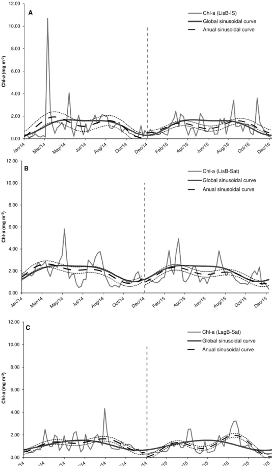
3.2.4. Comparison between the global sinusoidal curve and adjusted sinusoidal curves for two contrasting years (2014 and 2015)

Fig. 8 represents the weekly Chl-a data, the global sinusoidal curve for the 9-year period (hereafter named global model - solid lines), and

the sinusoidal curves adjusted separately for 2014 and 2015 in LisB and in LagB (hereafter named subset model – dash-dotted lines). These years were selected based on in situ Chl-a data in LisB (cf. Fig. 4A) as examples of years that contrast with the global model. The year 2014 had the highest record of biomass, while 2015 was characterized by having median values of Chl-a.

The main differences observed between the subset model and the global model in LisB for both datasets were the earlier observation of the Chl-a maximum in 2014 and the occurrence of a summer decline in 2014 and 2015 (Fig. 8A and B). This summer decline was more pronounced in 2015. In both years, the subset model suggests a bi-modal pattern, contrasting with the 5-months long period of high Chl-a values on the global model (Fig. 8A and B). Furthermore, for 2015, the in situ data showed a delay in the decreasing late-summer/early-winter trend (Fig. 8A). In general, the early-spring bloom peak was higher than the late-summer bloom peak in both years (Fig. 8A and B).

In LagB the subset model showed marked differences compared with the global model in 2014 and 2015 (Fig. 8C). Although more pro-nounced in 2015, two Chl-a peaks were recorded in both years, one in spring and the other in late-summer with a decrease in June. This con-trasts with the uni-modal global model that peaks in June (Fig. 8C). Contrasting with LisB, the late-summer bloom was higher than the spring bloom in LagB (Fig. 8C).

3.3. Cross-correlation structure between chlorophyll a estimated by satellite and meteorological and oceanographic variables

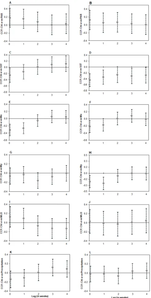
Fig. 9 shows the results of cross-correlation analyses between Chl-a and each MetOc variable, from lag 0 to lag 4 (0–4 weeks), during the winter/mid-spring period (Jan–Apr) in LisB and in LagB. During winter/ mid-spring a significant positive correlation between Chl-a and PAR was observed in both bays at lag 0 and 1, although stronger at lag 0 (Fig. 9A and B, Table B1). For this period, cross-correlation analyses did not show any other significant correlation between Chl-a and the remaining MetOc variables (SST, Mx, My, MLD and precipitation) (Fig. 9, Table B1).

The cross-correlation analyses, during the late-spring/summer period (May–Sep) in LisB and in LagB (Fig. 10, Table B2), showed a negative correlation between Chl-a and SST at lag 0 in both bays (Fig. 10C and D), but also at lag 1 in LagB, although this was weaker than at lag 0 (Fig. 10D). However, this correlation was only significant in LagB (Table B2).

Relative to Mx, a significant negative correlation with Chl-a was

found, which was stronger in LisB than in LagB (Fig. 10E and F,

Table B2). In both bays, this relationship was significant at lag 0, although in LisB it was also significant at lag 1. A significant negative correlation with Chl-a and My at lag 0 and 1 in LagB was also identified,

stronger at lag 1 (Fig. 10H, Table B2). For the late-spring/summer period, no other significant correlations were found between Chl-a and the remaining MetOc variables (PAR, MLD and precipitation in both bays, and My in LisB) (Fig. 10, Table B2).

4. Discussion

4.1. In situ chlorophyll a and ocean color products

Many remote sensing validation studies performed on the Portuguese continental coast have shown that satellite OC products produce acceptable estimates of in situ phytoplankton biomass, albeit with higher uncertainties in near-coast stations (Cristina et al., 2014, 2015; 2016; S´a et al., 2015). These studies focused on Chl-a estimates from the MERIS and MODIS instruments and on data products generated within the Ocean Color Climate Change Initiative (Cristina et al., 2014, 2015; 2016;

S´a et al., 2015). Correlations between remote sensing and in situ Chl-a can increase when obtained with a smaller spatial scale and a shorter temporal separation window (Caballero et al., 2014).

In the present study three different L4 datasets were used to perform

Fig. 6. Periodograms of the Chl-a time series: LisB-IS (A), LisB-Sat (B) and LagB-Sat (C). The graphs only show the results at timescales longer than one month.

(9)

a complementary assessment. Here, the aim was to identify the L4 OC product (which merges the results from several satellite products available for the region), available on the Copernicus Marine Environ-ment Monitoring Service, that presents the most similar temporal vari-ability pattern with the in situ data collected weekly. From the different analyzed products (Chl-CCI, Chl-GSM, Chl-OI), the Chl-OI product was the one that showed the highest correlation with the LisB near-coast in

situ station (r = 0.42) and the most similar Chl-a seasonal cycle (not

shown). Although the present correlation coefficient was weak compared to the ones obtained in the aforementioned studies, it should be noted that Sá et al. (2015), who studied several stations in the Central and North Portuguese coast, recorded the lower quality scores at the same nearshore station in LisB. According to these authors, the high temporal variability and the poor atmospheric correction in near-coast stations are factors that result in satellite overestimations. Here, despite the careful selection of the pixel to compare with the in situ data (cf. 2.3), the Chl-OI product was also found to overestimate in situ Chl-a concentrations especially in winter and spring months. This period coincided with the rainier months and subsequently with the increase in Tagus river runoff and turbidity (Fig. 2; Fernández-Nóvoa et al., 2017). Winds and the fortnightly spring–neap tidal cycle can also increase the turbid zone of rivers (Valente and da Silva, 2009). The high concen-tration of suspended matter present in a river plume induces a strong signal detected by the satellite, which may lead to overestimation of the Chl-a concentration (e.g. Fernández-Nóvoa et al., 2017 and references therein). Areas such as LisB, where optical variability throughout the year is high due to the near-coast location, the presence of a river plume and the frequent occurrence of upwelling filaments, are among the most challenging regions for the performance of satellite Chl-a estimates. Our results also evidenced that even when using the OC product that best fits the in situ Chl-a seasonal cycle, satellite estimates may reproduce an anticipation of the beginning and end of maximum Chl-a concentrations. The present work reinforces the need for further work to continue the search for better ocean color algorithms in these complex waters.

4.2. Phytoplankton biomass seasonality

In this study, the phytoplankton biomass dynamics was identified and characterized in two SW Iberian Bays, by using a similar approach to the one developed for NW Iberia (Beca-Carretero et al., 2019; Bode et al., 2011, 2019; Nogueira et al., 1997) and for the open ocean in the NE Atlantic (Bashmachnikov et al., 2013). The present 9-year time series analysis revealed a dominant 12-month cycle and a significant 6-month periodic component, agreeing with the results obtained by other authors for the NE Atlantic (Bashmachnikov et al., 2013; Beca-Carretero et al., 2019; Bode et al., 2019). This was also described by Winder and Cloern (2010), who studied 125 estuarine, coastal, lake and oceanic sites in the temperate and subtropical region and observed that the 12-month periodicity (spring bloom) was the most common Chl-a pattern, fol-lowed by the 6-month periodicity (bi-modal pattern). However, it should be noted that to account for the full variability of phytoplankton biomass it is important to consider some particular features, such as the non-stationarity (Winder and Cloern, 2010), the high interannual vari-ability (this study), and the spatial varivari-ability at a relatively small regional scale (Bode et al., 2011).

The present study showed that satellite Chl-a variability in Lisbon and Lagos Bays was characterized by a productive period from March/ April to August/September, agreeing with several recent studies per-formed on the Portuguese continental coast (Cabrita et al., 2015; Krug et al., 2017, 2018; Reboreda et al., 2014). The Chl-a sinusoidal curve indicated the presence of a uni-modal pattern in both bays, but with distinct features: LisB was characterized by high biomass over a long period, slightly higher in spring than in summer, and LagB was char-acterized by a symmetrical pattern with a clear maximum centered in June. This result contrasts with the bi-modal biomass pattern previously described for several regions in the West and South Portuguese coasts (Cabrita et al., 2015; Krug et al., 2017, 2018; Reboreda et al., 2014). These discrepancies may be related to the methodologies used to char-acterize the seasonal patterns. The above-mentioned studies analyzed phytoplankton biomass seasonal variability using a boxplot (or a similar

Fig. 7. Chl-a sinusoidal curves adjusted to the time series of LisB-IS, LisB-Sat and LagB-Sat for the period 2008–2016. Horizontal lines indicate the 60th _{percentile of}

each Chl-a data set. The dashed lines correspond to the standard errors of each sinusoidal curve.

(10)

Fig. 8. Comparison between weekly Chl-a data, global sinusoidal model by using the entire 9-years study period (solid line) and the subset models (dash-dotted lines) resulting from fitting sinusoidal curves for 2014 and 2015: LisB-IS (A), LisB-Sat (B) and LagB-Sat (C). The dashed lines correspond to the standard errors of the sinusoidal curves for 2014 and 2015.

(11)

Fig. 9. Cross-correlations functions (CCF) between Chl-a estimated by satellite and MetOc variables using satellite data for winter/mid-spring in LisB (left panel) and in LagB (right panel): Chl-a versus PAR (A and B); Chl-a versus SST (C and D); Chl-a versus Mx (E and F); Chl-a

versus My (G and H); Chl-a versus MLD (I and J); Chl-a

versus Precipitation (K and L). The dots represent the point estimates and the dashed lines show the lower and upper limits of the 90% CI for the CCF. For each lag, if the dashed line crosses the x-axis, the null hypothesis of no correlation between the time series is not rejected at the significance level.α ≤ 0.10.

(12)

Fig. 10. Cross-correlation functions (CCF) between Chl-

a estimated by satellite and MetOc variables using sat-ellite data for late-spring/summer in LisB (left panel) and in LagB (right panel): Chl-a versus PAR (A and B); Chl-a versus SST (C and D); Chl-a versus Mx (E and F); Chl-a

versus My (G and H); Chl-a versus MLD (I and J); Chl-a

versus Precipitation (K and L). The dots represent the point estimates, and the dashed lines show the lower and upper limits of the 90% CI for the CCF. For each lag, if the dashed line crosses the x-axis, the null hypothesis of no correlation between the time series is not rejected at the significance level.α ≤ 0.10.

(13)

graphical representation), which is an exploratory data analysis tool. In this work, a more precise methodology (in the sense that it allowed statistical inferences) was applied to describe the seasonal patterns of each Chl-a time series under consideration, namely the sinusoidal model.

The differences observed in Chl-a seasonal cycles patterns between both bays reflect distinct oceanographic processes affecting the biogeochemistry of each bay. The Tagus estuary drains nutrient-rich waters into LisB during winter/early-spring (Cabrita et al., 2015), which combined with the summer upwelling (Fig. 3E; Moita et al., 2003;

Oliveira et al., 2009b) allows for a long nutrient-rich period in this bay. By contrast, the absence of major rivers renders seasonal upwelling as the single primary nutrient source in LagB. Other factors such as dis-tance to the main upwelling centers (CR and CSV) and the prevailing wind regimes may also contribute to the observed differences.

On the central West coast, LisB was characterized by high Chl-a concentrations (maximum of 2.5 mg m-3_{) and three main biological}

seasons were identified based on phytoplankton biomass dynamics: (1) the early-winter/early-spring (December/early-March) characterized by a rapid increase in phytoplankton biomass, reaching maximum values in early-spring; (2) the early-spring/mid-summer (early-March/early- August) marked by sustained high phytoplankton biomass; and (3) the mid-summer/autumn (mid-August/November) with a steep decline in phytoplankton biomass. A previous study that analyzed the upwelling seasonality in this bay (Palma et al., 2010) suggested the presence of three upwelling seasons: (1) a transition period from downwelling to upwelling (February–May); (2) the upwelling season (June–September); and (3) the downwelling season (October–January). However, although the number of upwelling seasons is the same as the biomass seasons, the length, onset, and end of the seasons does not coincide.

On the South coast, LagB was characterized by relatively low Chl-a concentrations (maximum of 1.5 mg m-3_{) but three main biological}

seasons were also identified: (1) the early-winter-early/spring (December/March) marked by a slow steady increase in phyto-plankton biomass; (2) the mid-spring/summer (April/August) with a short maximum in June; and (3) the late-summer/autumn (September/ November) characterized by a slow decrease in biomass. This contrasts with the seasonal pattern identified by Goela et al. (2016) based on upwelling seasonality near CSV (close to LagB). These authors suggested the occurrence of four upwelling seasons for this region coinciding with the astronomical seasons: summer characterized by strong persistent upwelling, autumn by upwelling relaxation, and spring and winter by intermittent periods of upwelling.

The mismatch (in Lisbon) and the different number of seasons (in Lagos) between phytoplankton biomass seasons and those identified based on upwelling cycles highlights the need for explanatory drivers other than upwelling dynamics to better understand the phytoplankton biomass seasonal cycle on the West and South coasts of Iberia (see 4.3. for further discussion).

Another study performed further north in the West coast showed a long uni-modal Chl-a seasonal cycle characterized by high concentration values (4 mg m-3_{) but with a short peak in July/August (}_{Bode et al.,}

2011). At this site, the onset of the spring phytoplankton bloom was delayed 2-months relative to LisB and LagB, starting only in late-February/March. In the North coast of Iberia, coastal sites beyond Cape Finisterre and in Mar Cantabrico, less influenced by coastal up-welling and remineralization processes, were characterized by lower maximum Chl-a concentrations (0.5–2.5 mg m-3_{) and by a bi-modal}

pattern (spring and autumn blooms) (Bode et al., 2011).

The seasonal patterns of Chl-a described for the upwelling influenced Atlantic Iberian coast (Bode et al., 2011; this study) suggest a latitudinal trend changing from a clear uni-modal pattern in the South coast, to a uni-modal pattern characterized by high biomass over a long period in the West coast, and finally a bi-modal pattern in the North coast. A latitudinal increase in Chl-a concentration was also observed along the Western Iberian coast (this study; Bode et al., 2011; Ferreira et al.,

2019), agreeing with what has been previously described for this region (e.g. Carr, 2002; Chavez and Messi´e, 2009).

4.3. Relationship between chlorophyll a seasonal cycle and underlying meteorological and oceanographic drivers

Understanding the patterns and links between environmental drivers and phytoplankton biomass is not straightforward. Choosing the appropriate time scale is of special relevance to elucidate the relative contribution of local processes on phytoplankton dynamics. Here, cross- correlation analysis was used because it is a suitable tool to study the relationship between two time series. This technique allowed the quantification of the strength of the correlation between phytoplankton biomass and several MetOc variables for different oceanographic pe-riods (winter/mid-spring and late-spring/summer).

The winter/mid-spring period was characterized by the increase in PAR, low SST and shoaling of MLD. In both studied bays, the increase of Chl-a during this period was significantly correlated with the increase in PAR, which suggests light limitation during winter/mid-spring. The late- spring/summer period was characterized by the highest PAR values and by the increase and highest SST values. It was also the most favorable upwelling period with shallower MLD. In both bays, the high levels of Chl-a during late-spring/summer were significantly related with the increase in upwelling and the decrease in SST. The relevance of these drivers has been previously suggested for the Atlantic Iberian coast (e.g.

Ferreira et al., 2019; Krug et al., 2017, 2018; Moita, 2001; Oliveira et al., 2009a) and for other upwelling regions (Lamont et al., 2014; Walter et al., 2018).

Nevertheless, there were some differences between the two studied bays regarding the correlation between Chl-a and the two upwelling indices (Mx and My). In both bays, zonal transport showed a significant

negative correlation, stronger in LisB and at both lags 0 and lag 1-week, and weaker in LagB and significant only at lag 0. This highlights the relevance of intensity and persistence of seasonal upwelling for the high levels of phytoplankton biomass in LisB. This bay is located near CR coastal discontinuity (~12 Km distance) that influences the generation of upwelling coastal jets and associated recirculation cells. These fea-tures are known to favor the concentration of high phytoplankton biomass in this bay (Moita et al., 2003, Oliveira et al., 2009a, b). Meridional transport was only significant in LagB (at both lag 0 and lag 1-week) where it showed a stronger correlation than zonal transport due to the coastline orientation. LagB is located on the most western sector of the South coast of Iberia, close to the CSV upwelling center (~30 Km), where the West coast meets the South coast. This geographical setting explains the influence of upwelling generated by both the N–S and W-E wind component in this bay. Along this stretch of coast the occurrence of upwelling generated by the W-E wind component is usually described as occasional (e.g. Relvas and Barton, 2002). However, our results show that the intensity and persistence of upwelling that occur under westerly winds have a stronger influence on phytoplankton biomass in LagB than the upwelling filaments generated near CSV under northerly winds. Relative to SST, the decrease in SST associated with the occurrence of upwelling was stronger in LagB, where two different wind components were contributing to the observed decrease.

Similar correlations were found in recent studies between upwelling indices and Chl-a concentrations in the Atlantic Iberian coast (Ferreira et al., 2019; Krug et al., 2017, 2018). The main difference was that on the South coast these authors only found positive effects of the My, and

not of the Mx, over Chl-a. However, in Krug et al. (2017) results, LagB is

located close to the border that separates two distinct coastal regions in the South coast (cf. their Fig. 6): to the west, a region under major up-welling influence near CSV, where only the zonal transport is very significantly related with Chl-a; and to the east, a region under minor upwelling influence, where only the meridional transport appears as relevant to Chl-a. This particular location of LagB on an oceanographic border region may contribute to the importance of both upwelling

(14)

indices in our study. Another aspect is the different methodological approaches. To identify the relevant drivers for Chl-a variability we used Cross-Correlation Functions on a weekly scale. Ferreira et al. (2019) and

Krug et al. (2017, 2018) used Generalized Additive Models (GAMs) and longer time scales (e.g. monthly), which largely reduced the time dependence between observations. The results presented here highlight the need to consider the weekly time scale when investigating the pat-terns of phytoplankton biomass and its relation to highly variable oceanographic processes, such as upwelling. Thus, the choice of the time scale may play a determinant role in capturing the actual correlation between Chl-a and zonal and meridional transports.

In both studied bays the onset of the spring bloom (Fig. 7) seems to coincide with the deep MLD phase (Fig. 3) and the high biomass spring/ summer season described above (4.2) agrees with the MLD shoaling phase. However, no significant correlation was found between MLD and the annual Chl-a time series. In the last decade, MLD has been suggested as having different roles in phytoplankton biomass in the Iberian coast. Some authors report that MLD played an important role in defining the physical conditions for phytoplankton growth (Oliveira et al., 2009a), while others reported negative correlations between both datasets (Ferreira et al., 2019). It was also recently proposed that the timing of the spring bloom onset occurred during the MLD deepening phase and not during the MLD shoaling phase (Krug et al., 2017, 2018; Navarro et al., 2012; Reboreda et al., 2014). Other works have also questioned the long-standing interpretation of the critical depth hypothesis pro-posed by Sverdrup (1953) for the development of the phytoplankton spring bloom in the middle and high latitudes of the North Atlantic (see

Behrenfeld, 2010 and Fischer et al., 2014 for a review). The ecological disturbance-recovery hypothesis recently proposed by Behrenfeld (2010) may be a possible explanation for the absence of correlation between MLD and Chl-a concentrations in the present study. According to this view, blooms are initiated by physical processes that disrupt the predator-prey balanced interactions, such as deep winter mixing and low light, freshwater input or upwelling (Behrenfeld et al., 2013; Beh-renfeld and Boss, 2014). Further research designed to test this hypoth-esis, and other phytoplankton top-down controls, in coastal areas affected by seasonal upwelling will certainly contribute to a better un-derstanding of marine ecosystem functioning.

5. Conclusions

In this study, the phytoplankton biomass seasonal cycles obtained using 9 years of Chl-a datasets for Lisbon and Lagos Bays (West and South Atlantic Iberian coasts) indicate the existence of a latitudinal trend on Chl-a seasonal patterns along the upwelling influenced Atlantic Iberian coast. The westernmost South Iberian coast presents a uni-modal pattern with a short maximum centered in June and the central West coast, in the vicinity of a major river, has a uni-modal pattern charac-terized by high biomass over a long period, slightly higher in spring than in summer. Comparisons between in situ and satellite datasets performed in LisB revealed that even when using the OC product that best fitted with in situ Chl-a, there are still substantial differences when adjusting the sinusoidal model to the data. This highlights the importance of maintaining a regular in situ sampling and a judicious use of satellite estimates in near-coast upwelling centers.

Analyses of cross-correlations between different MetOc variables and Chl-a indicated that, apart from the seasonal availability of PAR, local processes dominate the phytoplankton variability on weekly timescales, namely upwelling and SST. Although with some differences between the bays these variables (PAR, SST and upwelling) presented a direct cor-relation with Chl-a at both lags 0 and lag 1-week and can be identified as drivers for triggering and maintaining phytoplankton biomass. Clear differences were observed in the role of the different wind components and SST in phytoplankton biomass dynamics in each bay. The relative importance of each wind component was determined by the coastline orientation at the study site and its distance to the main upwelling

centers. This work highlights the importance of choosing the appro-priate time scale to elucidate the relative contribution of local processes on phytoplankton distribution.

Declaration of competing interest

The authors declare that they have no known competing financial interests or personal relationships that could have appeared to influence the work reported in this paper.

Acknowledgements

Financial support of M. Santos was provided by a Portuguese PhD grant from FCT - Fundaç˜ao para a Ciˆencia e a Tecnologia (SFRH/BD/ 52560/2014). This work was financially supported by IPMA (MAR2020- P02M01-1490 P) and by FCT through UIDB/04292/2020, UID/Multi/ 04326/2020, UID/MAT/04561/2020 and project LISBOA-01-0145- FEDER-031265 co-funded by EU ERDF funds, within the PT2020 Part-nership Agreement and Compete 2020. The authors acknowledge as well the funding from the European Union’s Horizon 2020 Research and Innovation Programme grant agreement N 810139: Project Portugal Twinning for Innovation and Excellence in Marine Science and Earth Observation – PORTWIMS. A. Silva acknowledges funding from FCT (SFRH/BPD/63106/2009), IPMA (IPMA-BCC-2016-35) and project MarRisk (Interreg POCTEP Spain-Portugal, 0262 MARRISK 1 E).

The authors would like to express a special thanks to all the col-leagues at IPMA who helped with sample collection, fieldwork and laboratory support. This study has been conducted using E.U. Coperni-cus Marine Service Information products OCEAN-COLOUR_GLO_CHL_L4_REP_OBSERVATIONS_009_082 and 009_093 extracted from http://marine.copernicus.eu/.

Appendix A. Supplementary data

Supplementary data to this article can be found online at https://doi. org/10.1016/j.csr.2020.104200.

References

Alvarez, I., Gomez-Gesteira, M., DeCastro, M., Dias, J.M., 2008. Spatio temporal evolution of upwelling regime along the western coast of the Iberian Peninsula. J. Geophys. Res. 113 https://doi.org/10.1029/2008JC004744. C07020. Bashmachnikov, I., Belonenko, T.V., Koldunov, A.V., 2013. Intra-annual and interannual

non-stationary cycles of chlorophyll concentration in the Northeast Atlantic. Remote Sens. Environ. Times 137, 55–68. https://doi.org/10.1016/j.rse.2013.05.025.

Beca-Carretero, P.P., Otero, J., Land, P.E., Groom, S., ´Alvarez-Salgado, X.A., 2019. Seasonal and inter-annual variability of net primary production in the NW Iberian margin (1998–2016) in relation to wind stress and sea surface temperature. Prog.

Oceanogr. 178, 102135.

Behrenfeld, M.J., 2010. Abandoning sverdrup’s critical depth hypothesis on phytoplankton blooms. Ecology 91, 977–989. https://doi.org/10.1890/09-1207.1. Behrenfeld, M.J., Doney, S.C., Lima, I., Boss, E.S., Siegel, D.A., 2013. Annual cycles of

ecological disturbance and recovery underlying the subarctic Atlantic spring plankton bloom. Global Biogeochem. Cycles 27, 526–540. https://doi.org/10.1002/

gbc.20050.

Behrenfeld, M.J., Boss, E.S., 2014. Resurrecting the ecological underpinnings of ocean plankton blooms. Annu. Rev. Mar. Sci. 6, 167–194. https://doi.org/10.1146/

annurev-marine-052913-021325.

Behrenfeld, M.J., Boss, E.S., 2018. Student’s tutorial on bloom hypotheses in the context

of phytoplankton annual cycles. Global Change Biol. 24, 55–77.

Bode, A., Anad´on, R., Mor´an, X.A.G., Nogueira, E., Teira, E., Varela, M., 2011. Decadal variability in chlorophyll and primary production off NW Spain. Clim. Res. 48, 293–305. https://doi.org/10.3354/cr00935.

Bode, A., ´Alvarez, M., Ruíz-Villarreal, M., Varela, M.M., 2019. Changes in phytoplankton production and upwelling intensity off A Coru˜na (NW Spain) for the last 28 years. Ocean Dynam. 69, 861–873. https://doi.org/10.1007/s10236-019-01278-y.

Box, G.E.P., Jenkins, G.M., Reinsel, G.C., Ljung, G.M., 2016. Time Series Analysis:

Forecasting and Control, fifth ed. John Wiley & Sons, New Jersey.

Caballero, I., Morris, E.P., Prieto, L., Navarro, G., 2014. The influence of the Guadalquivir River on the spatio-temporal variability of suspended solids and chlorophyll in the Eastern Gulf of Cadiz. Mediterr. Mar. Sci. 15, 721–738. https://

doi.org/10.12681/mms.844.

Cabrita, M.T., Silva, A., Oliveira, P.B., Ang´elico, M.M., Nogueira, M., 2015. Assessing eutrophication in the Portuguese continental exclusive economic zone within the