Dissertation Report Master in Electrical Engineering
High Performance Position Control for Permanent
Magnet Synchronous Drives
Aurelio Antonio Pesántez Palacios
Dissertation Report Master in Electrical Engineering
High Performance Position Control for Permanent
Magnet Synchronous Drives
Aurelio Antonio Pesántez Palacios
Dissertation/Report developed under the supervision of Doctor Luís Neves, professor at the School of Technology and Management of the Polytechnic Institute of Leiria and co-supervision of Engineer Rodrigo Sempértegui, professor at the Faculty of Engineering of the University of Cuenca.
ii This page was intentionally left blank
iii
Dedication
I would like to dedicate this dissertation
to my beloved parents
iv This page was intentionally left blank
v
Acknowledgements
I would like to thank SENESCYT, University of Cuenca and Polytechnic Institute of Leiria for the given opportunity to study and obtain my master’s degree.
I also would like to thank Prof. Luís Neves and Ing. Rodrigo Sempertegui, for the guidance and support provided during the elaboration of this work.
vi This page was intentionally left blank
vii
Resumo
Na conceção e teste de sistemas de controlo de acionamento elétrico, as simulações por computador fornecem uma maneira útil de verificar a correção e a eficiência de vários esquemas e algoritmos de controlo, antes de proceder à construção do sistema final, portanto, reduzindo assim o tempo de desenvolvimento e os custos associados. No entanto, a transição da fase de simulação para a implementação real deve ser tão direta quanto possível. Este documento apresenta o design e a implementação de um sistema de controlo de posição para maquinas síncronas de ímanes permanentes, incluindo uma revisão e comparação de vários trabalhos relacionados sobre sistemas de controlo não-lineares aplicados a este tipo de máquinas. O sistema geral de controlo de acionamento elétrico foi simulado e testado no software Proteus VSM que é capaz de simular a interação entre o firmware a implementar num microcontrolador e os circuitos analógicos a ele ligados. O dsPIC33FJ32MC204 foi usado como o processador de destino para implementar os algoritmos de controlo, e o modelo da máquina elétrica foi desenvolvido a partir de elementos genéricos existentes na biblioteca Proteus VSM. Como em qualquer sistema de acionamento elétrico de alto desempenho, aplicou-se um controlo orientado a fluxo magnético para alcançar uma regulação precisa de binário. O sistema de controlo completo é distribuído em três malhas de controlo, nomeadamente binário, velocidade e posição. Foram implementados e testados um sistema de controlo PID padrão e um sistema de controlo híbrido baseado em lógica difusa. Foram também simuladas a variação natural dos parâmetros do motor, como a resistência do enrolamento e o fluxo magnético. As comparações entre os dois esquemas de controlo foram realizadas para controlo de velocidade e posição, usando diferentes medidas de erro tais como o integral de erro quadrático, o integral de erro absoluto e o erro quadrático médio. Os resultados da comparação mostram um desempenho superior do controlador híbrido baseado em lógica fuzzy ao lidar com as variações dos parâmetros e reduzindo a ondulação de binário, mas os resultados são invertidos quando ocorrem distúrbios de binario periódicos. Finalmente, os controladores de velocidade foram implementados e avaliados fisicamente num banco de ensaio, embora baseado num motor DC sem escovas, com os algoritmos de controlo implementados num dsPIC30F2010, sendo os resultados consistentes com a simulação.
Palavras-chave: prototipagem de acionamentos elétricos, máquinas de íman
permanente, controlo de velocidade e posição, Proteus VSM, dsPIC30F / 33F, sistema de controlo difuso.
viii This page was intentionally left blank
ix
Abstract
In the design and test of electric drive control systems, computer simulations provide a useful way to verify the correctness and efficiency of various schemes and control algorithms before the final system is actually constructed, therefore, development time and associated costs are reduced. Nevertheless, the transition from the simulation stage to the actual implementation has to be as straightforward as possible. This document presents the design and implementation of a position control system for permanent magnet synchronous drives, including a review and comparison of various related works about non-linear control systems applied to this type of machine. The overall electric drive control system is simulated and tested in Proteus VSM software which is able to simulate the interaction between the firmware running on a microcontroller and analogue circuits connected to it. The dsPIC33FJ32MC204 is used as the target processor to implement the control algorithms. The electric drive model is developed using elements existing in the Proteus VSM library. As in any high performance electric drive system, field oriented control is applied to achieve accurate torque control. The complete control system is distributed in three control loops, namely torque, speed and position. A standard PID control system, and a hybrid control system based on fuzzy logic are implemented and tested. The natural variation of motor parameters, such as winding resistance and magnetic flux are also simulated. Comparisons between the two control schemes are carried out for speed and position using different error measurements, such as, integral square error, integral absolute error and root mean squared error. Comparison results show a superior performance of the hybrid fuzzy-logic-based controller when coping with parameter variations, and by reducing torque ripple, but the results are reversed when periodical torque disturbances are present. Finally, the speed controllers are implemented and evaluated physically in a testbed based on a brushless DC motor, with the control algorithms implemented on a dsPIC30F2010. The comparisons carried out for the speed controllers are consistent for both simulation and physical implementation.
Keywords: electric drives prototyping, permanent magnet machines, position control, Proteus VSM, dsPIC30F/33F, fuzzy control system.
x This page was intentionally left blank
xi
Table of Contents
1. INTRODUCTION ... 1
2. LITERATURE REVIEW ... 3
2.1. Active Disturbance Rejection Control ... 3
2.2. Backstepping Control ... 4
2.3. Backstepping Control with Particle Swarm Optimization ... 5
2.4. Model Reference Adaptive Control ... 5
2.5. Dynamic Inversion Control ... 6
2.6. Fuzzy Logic Model Reference Adaptive Control ... 6
2.7. Control using Artificial Neural Networks ... 7
2.8. Sliding Mode Control ... 8
2.9. Hybrid Model Reference Adaptive Control ... 9
2.10. Summary ... 10
3. CONTROL SYSTEM DESIGN FOR PMSM DRIVES ... 13
3.1. Mathematical model of Permanent Magnet Synchronous Machines ... 13
3.1.1. Representation in Stationary Reference Frame 𝜶 − 𝜷 ... 14
3.1.2. Representation in Rotating Reference Frame 𝒅 − 𝒒 ... 14
3.1.3. Electromagnetic Torque ... 16
3.1.4. Complete Model of PMSM in 𝒅 − 𝒒 reference frame ... 17
3.2. Standard PID Control System Design ... 17
3.2.1. PI Controller Design ... 18
3.2.2. PID Controller Design ... 20
3.2.3. Current Controller ... 22
3.2.4. Position Controller without Explicit Speed Control Loop ... 24
3.2.5. Position Controller with Intermediate Speed Control Loop ... 26
3.3. Hybrid Control System Design based on Fuzzy-Logic ... 29
3.3.1. Direct Fuzzy-Logic Position Controller ... 29
3.3.2. Fuzzy-Logic Position Controller with Proportional Action ... 31
3.3.3. Fuzzy Tuned PI Speed Controller ... 31
3.4. Practical Issues About Digital Control Implementation ... 35
3.4.1. Analog to Digital Acquisition and Filtering ... 35
3.4.2. Phase Delay and ZOH ... 36
3.4.3. Output Voltage Distortion due to Dead Time ... 36
3.4.4. Digital Signal Processing Delay ... 36
xii
4.1. Proteus VSM ... 37
4.2. PMSM Drive Model in Proteus VSM ... 37
4.2.1. Dynamic Stator Equivalent Circuits ... 37
4.2.2. Electromechanical Dynamic Equivalent Circuit ... 39
4.2.3. Integrator Circuit for Angular Position ... 40
4.2.4. Reference Frame Transformations ... 41
4.2.5. Inverter Model ... 43
4.3. dsPIC33FJ32MC204 and Interface Sensors ... 45
4.3.1. ADC Module and Simulated Current Sensor ... 45
4.3.2. Simulated Tachogenerator ... 45
4.3.3. Simulated Optical Encoder ... 46
4.3.4. Signal Conditioning Circuits ... 46
4.4. Space Vector PWM ... 46
4.4.1. Equations for turn-on Times ... 47
4.4.2. Voltage Limits ... 50
4.5. Standard PID Controllers Implementation ... 51
4.5.1. PI Current Controller ... 51
4.5.2. PI Speed Controller ... 52
4.5.3. P Position Controller ... 52
4.6. Fuzzy-Logic Controller Implementation ... 53
4.7. Parameters Variation ... 55
4.7.1. Stator Resistance Variation ... 55
4.7.2. Permanent Magnet Flux Variation ... 55
4.8. Simulation Results and Comparison ... 56
4.8.1. Current Control Loop ... 57
4.8.2. Speed Control Loop ... 57
4.8.3. Position Control Loop ... 58
4.8.4. Controllers Comparison ... 59
4.9. Practical Implementation for a BLDC motor ... 63
4.9.1. BLDC Motor Electrical Parameters Measurement ... 63
4.9.2. BLDC Motor Testbed ... 68
4.9.3. Torque Control with FOC Commutation ... 68
4.9.4. Torque Control with Trapezoidal Commutation ... 70
4.9.5. Speed Controllers Comparison ... 71
5. CONCLUSIONS ... 75
xiii
List of Figures
Figure 3.1 Block diagram of PI control system ... 18
Figure 3.2 Schematic diagram for current control of PMSM drives ... 22
Figure 3.3 Block diagram for angular position control without explicit speed control loop ... 26
Figure 3.4 Block diagram for angular position control with intermediate speed control loop ... 28
Figure 3.5 Direct fuzzy-logic position controller ... 29
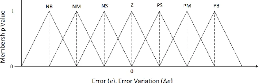
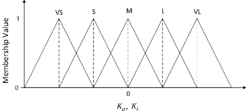
Figure 3.6 Input membership functions of the fuzzy-logic position controller ... 30
Figure 3.7 Output membership functions of the fuzzy-logic position controller ... 30
Figure 3.8 Fuzzy-logic position controller with proportional action ... 31
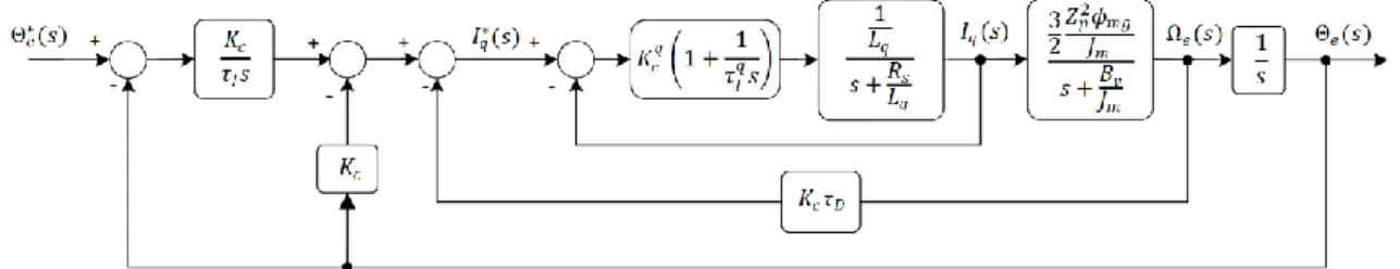
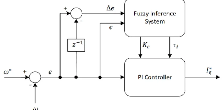
Figure 3.9 Block diagram for the fuzzy-tuned PI speed controller ... 32
Figure 3.10 Input membership functions for the fuzzy-tuned PI speed controller ... 32
Figure 3.11 Output membership functions for the fuzzy-tuned PI speed controller ... 33
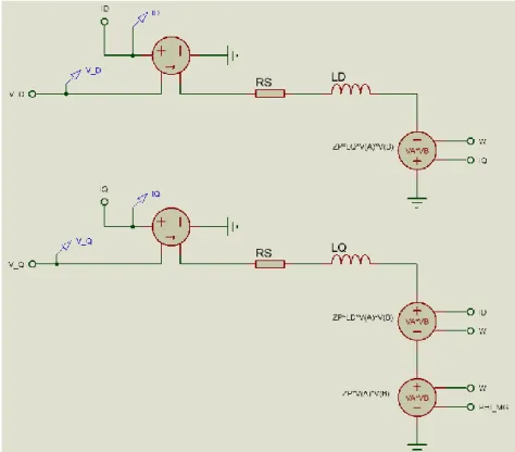
Figure 4.1 Dynamic stator equivalent circuits of the PMSM in the d-q reference frame37 Figure 4.2 Proteus multiplier voltage source element ... 38
Figure 4.3 Proteus implementation of dynamic stator equivalent circuits of PMSM in d-q reference frame ... 38
Figure 4.4 Parallel R-C circuit ... 39
Figure 4.5 Electromechanical dynamic equivalent circuit of the PMSM model ... 40
Figure 4.6 Integrator Circuit for Angular Position ... 40
Figure 4.7 Clarke's transformation ... 41
Figure 4.8 Park's transformation ... 42
Figure 4.9 Inverse Park's transformation ... 42
Figure 4.10 Inverse Clarke's transformation ... 43
Figure 4.11 Basic topology of a three-phase inverter ... 43
Figure 4.12 Three-phase inverter model ... 44
Figure 4.13 dsPIC33FJ32MC204 with emulated conditioning circuits ... 46
Figure 4.14 Principle of space vector modulation ... 47
Figure 4.15 Voltage constraint for linear modulation ... 50
Figure 4.16 Rectangular approximation constraint ... 50
Figure 4.17 Example of input fuzzification ... 53
Figure 4.18 Stator resistance step variation model ... 55
Figure 4.19 Permanent magnet flux step variation model ... 56
Figure 4.20 PI current controller test ... 57
Figure 4.21 PI speed controller test ... 57
Figure 4.22 Fuzzy-tuned PI speed controller test ... 58
Figure 4.23 Response of proportional position controller ... 58
Figure 4.24 Response of fuzzy-logic position controller with proportional action ... 59
Figure 4.25 Comparison of speed controllers. ISE error indicator ... 60
Figure 4.26 Comparison of speed controllers. IAE error indicator ... 61
Figure 4.27 Comparison of speed controllers. RMS error indicator ... 61
Figure 4.28 Comparison of position controllers. ISE error indicator ... 62
Figure 4.29 Comparison of position controllers. IAE error indicator ... 62
Figure 4.30 Comparison of position controllers. RMS error indicator ... 62
Figure 4.31 Schematic diagram for synchronous inductance measurement ... 64
Figure 4.32 BLDC motor testbed ... 68
xiv
Figure 4.34 BLDC motor fuzzy-tuned PI speed controller response ... 72
Figure 4.35 Comparison of speed controllers. ISE error indicator ... 73
Figure 4.36 Comparison of speed controllers. IAE error indicator ... 73
xv
List of Tables
Table 2.1 Summary of the reviewed non-linear control methods for PMSM drives ... 12
Table 3.1 Rule-base for the fuzzy-logic position controller ... 30
Table 3.2 Rule-base for the fuzzy-tuned PI speed controller ... 34
Table 4.1 Switching states of inverter ... 46
Table 4.2 Output voltage of inverter ... 47
Table 4.3 Sector identification according to N for SVPWM ... 49
Table 4.4 Bandwidths and frequencies of the PMSM control loops ... 56
Table 4.5 Comparison data for speed controllers ... 60
Table 4.6 Comparison data for position controllers ... 61
Table 4.7 Measured values for back-EMF-constant calculation ... 65
xvi This page was intentionally left blank
xvii
List of Acronyms
ADRC Active disturbance rejection control ANN Artificial neural networks
BLDC Brush-less direct current motor
CRPWM Current regulated pulse width modulation ESO Extended state observer
PID Proportional, integral and derivative PMSM Permanent magnet synchronous motor PSO Particle swarm optimization
SVPWM Space vector pulse width modulation TSM Terminal sliding mode
xviii This page was intentionally left blank
1
1. INTRODUCTION
Advances in microprocessor technologies and embedded systems have made possible implementations of complex control algorithms which require intensive math computations. Moreover, the recent development in power electronics and semiconductor devices have given a way for AC electric drives to be used instead of DC motors in high-performance applications [1].
The permanent magnet synchronous motor (PMSM) has gained an important place in applications where high-performance speed and position control are required. Characteristics such as high mass-power ratio, high torque-inertia ratio, high power density, high efficiency, reduced maintenance, etc., make the PMSM an interesting choice in applications such as industrial robots, machining tools, electric vehicles, wind turbines, etc. [2] [3] [4] [5].
A widely used control method in high-performance AC drives, is field oriented control, also known as vector control. This approach allows to control the three-phase AC machine currents through a coordinated change in the supply voltage amplitude, phase and frequency [6]. Field oriented control allows to regulate an AC electric drive in a way similar to that of the separately exited DC machine, but maintaining all the benefits of AC machines [7].
The overall performance of an electric drive will depend not only on the accuracy and speed of the control, but also on the robustness of the controller to operate correctly even if there are significant external disturbances, uncertainties in motor parameters, and lack of precise mathematical models.
Machine parameters change dynamically with temperature variations, magnetic saturations, skin effect, etc. These changes may affect the performance of an electric drive. To deal with these drawbacks, nonlinear control techniques such as fuzzy-logic controllers, sliding mode controllers, adaptive controllers, neural network controllers and hybrid controllers have been developed.
This research deals with the design and implementation of a PMSM drive control system, considering two types of controllers namely: a conventional proportional-integral-derivative (PID) controller and a hybrid controller based on fuzzy logic. The PMSM drive system is simulated and tested using the software Proteus VSM, including the implementation of controllers, coded for a dsPIC33FJ32MC204 processor.
2 This dissertation is organized as follows:
Chapter 2 reviews the state of the art considering some researches about nonlinear control methods for PMSM drives. A summary table of the reviewed control methods is also presented with information about the implementation platform, estimated processing power and complexity.
In Chapter 3 the PMSM control system is designed, starting with the mathematical model of the machine. Standard PID-based controllers are designed for three control loops namely current, speed and position. The design for a controller with only current and position loop (without explicit speed loop) is also presented. Hybrid controllers based on fuzzy-logic are designed for the speed and position loops. The chapter ends pointing out some practical issues about implementation of digital controllers.
Chapter 4 presents the controllers implementation, including the PMSM model developed in Proteus VSM and the required interfacing circuits for the dsPIC33FJ32MC204 processor. An algorithm for the space vector PWM implementation is also presented. Stator resistance and permanent magnet flux variations are simulated adding suitable circuits into the Proteus model. Simulation results and comparisons performed for various operating conditions are presented. The chapter finalizes giving details about the physical implementation of the speed controllers (PID and fuzzy) for a brushless DC motor (BLDC), with respective results and comparison.
3
2. LITERATURE REVIEW
A modern electric drive system is generally composed of several parts such as driven mechanical system, electric machine, power electronic converter, digital/analog controller, sensors/observers, and so on. With the current development in the field of power electronics and embedded systems technologies, there is a tendency of using AC machines instead of DC machines for electric drive systems [8].
Improvements in magnetic materials and motor fabrication technologies have made AC synchronous machines with permanent magnet excitation, interesting solutions for electric drive applications due to their special characteristics [9]; namely:
• There are no excitation losses which means substantial increase in efficiency. • Higher power density than synchronous motors with electromagnetic
excitation.
• High torque/inertia ratio.
• Higher magnetic flux density in the air gap. • Better dynamic performance.
• Compact size.
• Simplification of construction and maintenance.
In high performance drive systems, precise control with fast dynamic response and good steady state response are mandatory. Furthermore, unmodeled dynamics, external disturbances, and parameter variations have to be taken into account in a high performance electric drive system.
High performance control of permanent magnet synchronous motors has been addressed by many researchers using different non-linear control techniques. Some of these non-linear control implementations and their characteristics are described below.
2.1. Active Disturbance Rejection Control
The Active Disturbance Rejection Control (ADRC) uses an estimation/cancellation strategy to cope with disturbances both internal and external. The strategy is to use the measured information of the output of the system to estimate the total disturbance (internal unmodeled dynamics and external perturbations). An extended state observer (ESO), which takes into account not only the states but also the total disturbance, is used to estimate the required states. Once the disturbance estimation is complete, it is used in the feed-back loop, cancelling the total disturbance of the system. This cancellation
4 leads to a time invariant linear system which can be treated with conventional control theory [10].
A position control of PMSM using an active disturbance rejection controller had been proposed by Xing-Hua Yang et al., (2010), which is a disturbance rejection technique designed without an explicit mathematical model of the plant. In this reference work, field oriented control is applied to maximize torque. PI controllers are used for the current loops and the ADRC controller is applied in the position loop. A comparison study between a standard PID controller and the proposed ADRC controller is carried out by means of computer simulation with MATLAB/Simulink software, showing that both controllers have good performance but the ADRC controller leads to a smaller error and a faster response. An experimental verification of the proposed controller is applied using a TMS320F2812 DSP chip to implement the control algorithm. Satisfactory performance is obtained when the parameters of the controller are selected according to the maximum allowable overshoot and the required speed response of the system [11].
2.2. Backstepping Control
The backstepping is a systematic and recursive design methodology for nonlinear feedback control. The main idea behind this technique is to recursively select appropriate functions of state variables as pseudo-control inputs for lower dimension subsystems. In other words, starting with a known-stable subsystem, outer subsystems can be designed expressed in terms of the inner ones. When the procedure terminates, a feedback design for the whole system is obtained. The system is designed with the desired characteristics and stability using a recursive Lyapunov-based scheme [12].
Kendouci Khadija et al., (2010), had presented a speed tracking control of PMSM using a backstepping control technique based on feedback laws and Lyapunov stability theory. In this reference work, an extended Kalman filter observer is applied to estimate the rotor speed which is feedback controlled by the backstepping control strategy. Field oriented control is applied, the d-axis current command is set to zero to maximize the torque production. The performance of the proposed backstepping sensorless speed control is evaluated by computer simulation using MATLAB/Simulink software. An experimental validation of the control algorithm is also carried out in a test-bed using the dSPACE 1103 control board. Results show that the system can track speed step references with acceptable performance, although, a large ripple is present even for considerable speeds (1000 rpm) [13].
5
2.3. Backstepping Control with Particle Swarm Optimization
Particle swarm optimization PSO refers to a metaheuristic that imitates the nature process of group communication to share individual experiences. PSO allows to optimize a problem starting with a possible population of solutions named “particles”. These particles are moved across the entire search space based on mathematical rules that consider the position and speed of the particles. The movement of every particle is influenced by its better local position found so far, as well as by the better global positions found by other particles as they travel through the search space [14].
Ming Yang et al., (2010), present an improved proposal for controlling the speed of a PMSM based on the backstepping technique with the addition of an adaptive weighted particle swarm optimization (PSO). The PSO is used to optimize the controller parameters, adding robustness to the control system. The proposed control strategy is tested by means of computer simulation. A comparative study between the normal backstepping-based controller and the PSO-based backstepping controller is performed. Results show that the proposed adaptive weighted PSO has better dynamic and steady state performance than the normal backstepping-based controller [15].
2.4. Model Reference Adaptive Control
The idea behind the model-reference adaptive control technique is to develop a closed loop controller with parameters that can be modified to change the response of the system. The desired response of the process to a signal input is specified as a reference model. The output of the process is compared with the output of the reference model to generate an error signal. An adaptation mechanism looks at this error and calculates the adequate parameters for the main controller in order to minimize the error. Lyapunov’s stability and Popov’s hyperstability theories are standard design methods for the control law in adaptive control systems [16].
Liu Mingji et al., (2004) had proposed a position control for PMSM using a model reference adaptive control scheme. Popov’s hyperstability theory is applied for designing the adaptive control law in the position loop. A current regulated pulse with modulation (CRPWM) technique is used for controlling the voltage source inverter that feeds the motor. A velocity observer is used to estimate the velocity of the motor shaft. The controller is implemented on an industrial computer and the results show that the output of the system follows the output of the reference model with acceptable performance despite uncertainties and parameter variations [17].
6
2.5. Dynamic Inversion Control
Dynamic inversion technique uses a virtual control input that allows to control a nonlinear system in a simple linear way. The strategy is to rewrite the state space system in its companion form in such way that all the nonlinear terms only affect the last state-space variable. The virtual control input is then defined in terms of the last state space elements. To clarify, consider the following nonlinear dynamic system [18]
𝒙̇ = 𝑓(𝒙) + 𝑔(𝒙)𝑢
𝑓(𝑥) and 𝑔(𝑥) can be nonlinear functions. The companion form of this model will be
[ 𝑥1̇ ⋮ 𝑥𝑛−1̇ 𝑥𝑛̇ ] = [ 𝑥2 ⋮ 𝑥𝑛 𝑏(𝒙) ] + [ 0 ⋮ 0 𝑎(𝒙) ] 𝑢
As can be seen, all the nonlinear terms only affect 𝑥𝑛. The virtual control input 𝑣 is defined as
𝑣 = 𝑏(𝒙) + 𝑎(𝒙)𝑢
The input of the system in terms of the virtual control input is 𝑢 = 𝑎−1(𝒙)(𝑣 − 𝑏(𝒙))
The virtual control input 𝑣 can now be used to control the entire system in a linear way. Zhang Yaou, et al., (2010) propose a velocity control of PMSM based on the dynamic inversion approach. The controller is designed with a structure similar to a conventional PI cascade control system. The dynamic inversion is applied separately to the low frequency (velocity loop) and to the high frequency (current loop) dynamics of the system. The proposed controller is tested in terms of computer simulations using MATLAB/Simulink software. A step speed command is applied and tested for three different load torques. Acceptable performance is obtained with a good steady state response for all cases [19].
2.6. Fuzzy Logic Model Reference Adaptive Control
Basically, Fuzzy Logic is a multilevel logic that allows to define intermediate values when evaluating a statement. It is an attempt to catch and represent the human knowledge. In fuzzy logic, an affirmation can be truth for many degrees of truth, from completely true to completely false [20].
Nowadays, fuzzy logic is widely applied in control systems. A fuzzy logic controller will use fuzzy membership functions and inference mechanisms to determine the appropriate control signal. Fuzzy-logic-based controllers are usually applied together with other types of controllers/systems to achieve better performances [21].
7 Mohamed Kadjoudj et al., (2007), propose a model reference adaptive scheme to control the speed of a PMSM in which the adaptation mechanism uses the error and the variation of the error between the output of the reference model and the output of the system as inputs for a fuzzy-based adaptation mechanism. The main controller is also a fuzzy-logic controller whose rule base and inference mechanism are modified according to the adaptation mechanism. A comparison among the proposed fuzzy-logic adaptive controller, stand-alone fuzzy-logic controller and a fixed gain PI controller is performed using computer simulations with the MATLAB/Simulink software. Results show that the proposed fuzzy-logic adaptive controller has better performance when a repetitive step change in load torque is applied [22].
Ying-Shieh Kung and Pin-Ging Huang (2004), had presented a high-performance position controller for PMSM using a fuzzy-logic controller in the position control loop with and adaptation mechanism based on the gradient method. Vector control is applied setting the d-axis current reference to zero. PI controllers are used for the current control loop. Space vector pulse width modulation (SVPWM) is applied as a modulation technique to control the inverter. The overall system, including the adaptive controller and the SVPWM scheme are implemented in a TMS320F2812 DSP chip taking advantage of its processing power and peripheral availability. Experimental results demonstrate that in step command response and frequency command response, the rotor position rapidly tracks the prescribed dynamic response, thus, obtaining a high-performance position controller for PMSM drives [23].
2.7. Control using Artificial Neural Networks
Artificial neural networks (ANN) are non-linear processing information devices that are constituted by elementary processing devices interconnected to each other, the so-called neurons. The basic building blocks that constitute an artificial neural network are: network architecture, weights determination, and activation functions. The way in which neurons are arranged in layers and interconnection patterns, within and inside of those layers, is called the network architecture. There are many types of neural network architectures namely, feed forward, feedback, fully interconnected net, competitive net, etc. Neural networks use hidden units to enhance the internal representation of input patterns [24].
Mahmoud M. Saafan et al., (2012) present a neural network controller for PMSM. Two methods are proposed, the first one is the application of a neural-network-based controller for the speed loop and the second one is a neural-network-based torque
8 constant and stator resistance estimator. In both cases, the neural network is used to minimize torque ripple. The neural network weights are initially chosen randomly with small values, then, a model reference control algorithm is applied to adjust those weights to optimal values. A feed-forward neural-network architecture is applied for the parameter estimation strategy in the second method. The proposed control schemes are tested by means of computer simulation using MATLAB/Simulink software. Results show good performance with no speed overshoot. Furthermore, the obtained torque ripple values are compared with the torque ripple percentages given in other publications, observing an improved torque ripple reduction with the proposed methods [25].
2.8. Sliding Mode Control
Sliding mode control is a nonlinear control method whose purpose is to alter the dynamic of a nonlinear system applying a discontinuous control signal that force the system to “slide” along a defined state-space trajectory. The intrinsic discontinuous characteristic of the sliding mode allows a simple control that can be designed to switch between only two states (on/off) without a precise definition, therefore, adding robustness against parameter variations. A drawback of sliding mode is the introduction of high frequency oscillations around the sliding surface that strongly reduces the control performance. The aforementioned drawback is the so-called chattering effect which has to be taken into account in high performance control system implementations [26].
Fadil Hicham et al., (2015) present a velocity control of PMSM based on the sliding-mode along with a fuzzy-logic system for chattering minimization. The sliding mode controller is applied to the velocity control loop. PI controllers with decoupling compensations are applied to the current control loop. To deal with the chattering effect, a fuzzy logic controller is implemented based on the calculation of a mitigating term which will be multiplied by the discontinuous component of the sliding-mode controller. The proposed system is tested by means of computer simulations using the software tool PLECS integrated with MATLAB/Simulink. The controller is also implemented in a eZdspF28335 board using MATLAB/Simulink rapid prototyping to control an 80W PMSM. Both the sliding mode controller and the fuzzy-logic sliding mode controller were tested obtaining similar dynamic responses but verifying the effectiveness of the fuzzy-logic sliding mode controller to reduce the chattering effect [27].
Fouad Giri (2013) presents a high order terminal sliding mode control (TSM) with mechanical resonance suppressing for PMSM servo systems. TMS manifolds are designed for stator currents and load speed, respectively, to ensure convergence in finite time and obtain better tracking precision. A full-order state observer is applied to estimate
9 the load speed and the shaft torsion angle which cannot be measured directly. To evaluate the proposed sliding-mode based mechanical resonance suppressing method, some computer simulations with MATLAB are carried out. The step response of the motor speed is compared for three different mechanical resonance suppressing methods, namely, notch filter, acceleration feedback, and TSM control. Results show that the response of the notch filter is faster compared to other two methods. The effect of suppressing mechanical resonance using the acceleration feedback is better than the notch filter. The effect of suppressing mechanical resonance using the TMS control is the better compared to the other two methods. The speed response time of the TSM control is similar to the notch filter [28].
2.9. Hybrid Model Reference Adaptive Control
Various control techniques can be applied together in order to obtain an enhanced control performance. A hybrid position controller for PMSM conformed by three main controllers namely, an adaptive fuzzy-logic-neural-network controller, a robust controller and an auxiliary controller based on the sliding mode had been proposed by Fayez F.M. El-Sousy (2014). This complex controller is designed in order to guarantee stability and high-performance operation of the PMSM and to eliminate the need of having a prior knowledge of the constrain conditions of the system, thus, increasing the portability of the controller to other nonlinear dynamic systems. In this proposal, a decoupled current control loop is implemented with PI controllers for the d-axis and q-axis currents. To maximize torque, d-axis current reference is forced to be zero. The adaptive hybrid controller is applied to the position loop, skipping the velocity loop and thus, giving the torque reference directly from the position controller to the torque controller. The experimental validation of the proposed tracking control scheme is carried out using the MATLAB/Simulink package and a DSP control board dSPACE DS1102 based on TMS320C31 and TMS320P14 DSP chips installed in the control desktop computer. To investigate the robustness of the proposed controllers, four cases including parameter uncertainties and external load disturbances are considered. The experimental results successfully confirm that the proposed adaptive hybrid control system grants robust performance and precise dynamic response to the reference model regardless of the PMSM parameter variations and load disturbances [29].
10
2.10. Summary
As can be seen, there are various nonlinear control techniques which can be applied to cope with uncertainties and parameter variations in PMSM drive systems. Most of the reviewed PMSM control systems are implemented and tested with the help of MATLAB/Simulink software. Some experimental validations are also carried out in PMSM testbeds. The real-world implementations are performed using MALTAB/Simulink code generation capability in some cases, and direct coding in some others. For all the reviewed real-world implementations, high-end powerful hardware is used to execute the control algorithms.
Although there is not a direct way to determine the relationship between a specific control algorithm and the amount of processing power required to execute it, having a way to experiment and estimate that relationship will be helpful for selecting the hardware and the control strategy which better fit to a specific application.
Furthermore, it is not always practical/possible to test the controllers within a real-world testbed. For instance, if different hardware platforms need to be considered/compared, or if a change in hardware is required, a computer simulation of these scenarios will reduce costs and implementation time. Nevertheless, a straightforward transition from the computer simulation to the real-world implementation is required.
Another point to be noted in the reviewed literature is the PMSM model used for the simulations. In all cases, the PMSM model considers balanced stator windings with sinusoidal distributed magnetomotive force, sinusoidal inductance vs position, and neglects saturation and parameter changes.
To validate a control algorithm in terms of computer simulation, the model used to represent the plant/process must be as accurate as possible to obtain consistent results. The PMSM model used in the reviewed literature has sufficient characteristics for most initial designs, but the controller will require further adjustment/calibration to be performed in the real-world implementation. Nevertheless, a more realistic PMSM model will be required to catch the effects and performance of controllers implemented by means of computer simulation.
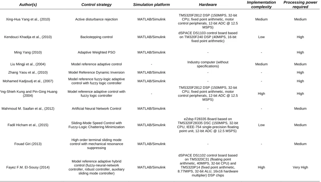
A summary of the reviewed non-linear control methods for PMSM drive systems is presented in table 2.1, including an estimation of the relative complexity and power processing capability required to implement the controller in each case. The processing power estimations are based on the number of calculations that need to be performed, paying special attention to divisions. The estimation of the implementation complexity
11 considers the hardware and software used to implement each specific controller. For instance, an implementation using a control board with MATLAB/Simulink support for code generation, will be easier than an implementation in a stand-alone controller via hand-written firmware.
12
Author(s) Control strategy Simulation platform Hardware Implementation complexity
Processing power required
Xing-Hua Yang et al., (2010) Active disturbance rejection MATLAB/Simulink
TMS320F2812 DSP (150MIPS, 32-bit CPU, fixed point arithmetic, motor control peripherals, 12-bit ADC @ 12.5
MSPS)
Medium Medium
Kendouci Khadija et al., (2010) Backstepping control MATLAB/Simulink
dSPACE DS1103 control board based on TM320F240 DSP (40MIPS, 16-bit
fixed point arithmetic)
Low High
Ming Yang (2010) Adaptive Weighted PSO MATLAB/Simulink - - High
Liu Mingji et al., (2004) Model reference adaptive control - Industry computer (without
specifications) Medium Medium
Zhang Yaou et al., (2010) Model Reference Dynamic Inversion MATLAB/Simulink - - High
Mohamed Kadjoudj et al., (2007) Model reference fuzzy-logic adaptive
control with fuzzy logic controller MATLAB/Simulink - - High
Ying-Shieh Kung and Pin-Ging Huang (2004)
Model reference adaptive control with
fuzzy logic controller -
TMS320F2812 DSP (150MIPS, 32-bit CPU, fixed point arithmetic, motor control peripherals, 12-bit ADC @ 12.5
MSPS)
High High
Mahmoud M. Saafan et al., (2012) Artificial Neural Network Control MATLAB/Simulink - - Medium
Fadil Hicham et al., (2015) Sliding-Mode Speed Control with
Fuzzy-Logic Chattering Minimization MATLAB/Simulink
eZdsp F28335 Board based on TMS320F28335 DSC (150MIPS, 32-bit CPU, IEEE-754 single-precision floating point unit, 12-bit ADC @ 12.5 MSPS)
Low Medium
Fouad Giri (2013)
High order terminal sliding mode control with mechanical resonance
suppressing
MATLAB/Simulink - - Medium
Fayez F.M. El-Sousy (2014)
Model reference adaptive hybrid control (fuzzy-neural-network controller, robust controller, auxiliary
sliding mode controller)
MATLAB/Simulink
dSPACE DS1102 control board based on TMS320C31 (floating point arithmetic, 40MIPS, 32-bit CPU) and
TMS320P14 (fixed point arithmetic, 8.77MIPS, 32-bit ALU, 16x16 hardware
multiplier) DSP chips
High Very High
13
3. CONTROL SYSTEM DESIGN FOR PMSM DRIVES
The control architecture of a high-performance electric drive system, designed to track a position reference, is composed for at least two control loops disposed in a cascade fashion. The current/torque controller will be in the inner-most loop, which is required to add robustness against stator resistance sensitivity. In addition, the torque loop will facilitate velocity control due to the intrinsic relationship between torque and acceleration. The intermediate control loop can be a speed controller, which helps to minimize the effects due to temperature sensitivity of the permanent magnets. The final control objective is accomplished by a position controller, which conforms the outermost loop of the overall control system. If only two-loops are considered, the explicit intermediate speed-loop is replaced by a more complex position controller.
This chapter includes the mathematical model of the PMSM machine, and presents the design of all the controllers required in a position tracking drive system. Conventional PID controllers, as well as fuzzy-logic based controllers are designed.
3.1. Mathematical model of Permanent Magnet Synchronous Machines
Obtaining a suitable dynamic model is the starting point to design and analyze any control system. The PMSM dynamic model is obtained considering the fundamental relationship between stator voltages and currents, expressed in the space phasor form. The procedure followed to obtain the PMSM mathematical model is based on reference [30]. Considering a three-phase machine with balanced three-phase currents given by
𝑖𝑎(𝑡) = 𝐼𝑠cos(𝜔𝑡 + 𝜙) 𝑖𝑏(𝑡) = 𝐼𝑠cos (𝜔𝑡 + 𝜙 −2𝜋 3) 𝑖𝑐(𝑡) = 𝐼𝑠cos (𝜔𝑡 + 𝜙 − 4𝜋 3 )
Where 𝜔 is the phase current frequency, 𝜙 is the initial angle, and 𝐼𝑠 is the amplitude. The space vector representation of the three-phase stator current can be written as
𝑖𝑠 ⃗⃗ =2 3[𝑖𝑎(𝑡) + 𝑖𝑏(𝑡)𝑒 𝑗2𝜋3 + 𝑖 𝑐(𝑡)𝑒𝑗 4𝜋 3] 𝑖𝑠 ⃗⃗ = 𝐼𝑠𝑒𝑗(𝜔𝑡+𝜙)
And the space vector representation of the three-phase stator voltage 𝑣𝑠 ⃗⃗⃗ =2 3[𝑣𝑎(𝑡) + 𝑣𝑏(𝑡)𝑒 𝑗2𝜋3 + 𝑣 𝑐(𝑡)𝑒𝑗 4𝜋 3]
14 Assuming that 𝜑⃗⃗⃗⃗ is the space vector representation of the stator flux linkage, the stator 𝑠 voltage equation of the machine is
𝑣𝑠
⃗⃗⃗ = 𝑅𝑠𝑖⃗⃗ +𝑠 𝑑𝜑⃗⃗⃗⃗ 𝑠
𝑑𝑡 (3.1)
Where 𝑅𝑠𝑖⃗⃗ is the voltage drop across the equivalent stator resistance, and 𝑠 𝑑𝜑⃗⃗⃗⃗⃗ 𝑠 𝑑𝑡 is the
induced voltage due to magnetic flux variations.
3.1.1. Representation in Stationary Reference Frame (𝜶 − 𝜷)
Projecting the three phase space vectors of the voltage and currents onto the real (𝛼) and imaginary (𝛽) axes, these vectors can be represented by complex notations as follows
𝑣𝑠
⃗⃗⃗ = 𝑣𝛼+ 𝑗𝑣𝛽 𝑖𝑠
⃗⃗ = 𝑖𝛼+ 𝑗𝑖𝛽
The relationship between the three-phase variables and the 𝛼 − 𝛽 variables is given by the Clarke transformation as follows
[ 𝑥𝛼 𝑥𝛽 𝑥0 ] =2 3 [ 1 −1 2 − 1 2 0 √3 2 − √3 2 1 2 1 2 1 2 ] [ 𝑥𝑎 𝑥𝑏 𝑥𝑐 ] The coefficient 2
3 is used to guarantee the energy conservation. The 𝑥0 term represents
the zero-sequence component of the three-phase system. For a balanced three-phase system, the 𝑥0 term is zero.
The inverse Clarke transformation is defined as
[ 𝑥𝑎 𝑥𝑏 𝑥𝑐 ] = [ 1 0 1 −1 2 √3 2 1 −1 2 − √3 2 1] [ 𝑥𝛼 𝑥𝛽 𝑥0 ]
The voltage and current variables in the α-β reference frame are still sinusoidal because of the direct relationship established by the Clarke transformation.
3.1.2. Representation in Rotating Reference Frame (𝒅 − 𝒒)
Rotating the space vector in 𝛼 − 𝛽 reference frame clockwise by 𝜃𝑒, the 𝑑 − 𝑞 reference frame is obtained. In this reference frame, the direct axis 𝑑 is always aligned with the rotating flux produced by the permanent magnets of the rotor, and the 𝑞 axis is in
15 quadrature. Because the rotor runs at the same speed as the supplying frequency at steady-state, this reference frame is also called the synchronous reference frame. Mathematically, the rotation of the space vectors is translated into multiplication by the factor 𝑒−𝑗𝜃𝑒, which leads to a set of new space vectors 𝑣
𝑠
⃗⃗⃗ ′, 𝑖⃗⃗ 𝑠′ denoting the space vectors referred to synchronous 𝑑 − 𝑞 reference frame. Projecting the transformed space vectors into the real and imaginary axes, the current and voltage variables in the 𝑑 − 𝑞 reference frame are
𝑣⃗⃗⃗ 𝑠′ = 𝑣⃗⃗⃗ 𝑒𝑠 −𝑗𝜃𝑒 = 𝑣
𝑑+ 𝑗𝑣𝑞 (3.2)
𝑖⃗⃗ 𝑠′ = 𝑖⃗⃗ 𝑒𝑠 −𝑗𝜃𝑒 = 𝑖
𝑑+ 𝑗𝑖𝑞 (3.3)
Similar, the stator flux can also be represented in the 𝑑 − 𝑞 frame by rotating the flux vector clockwise by 𝜃𝑒, leading to
𝜑𝑠
⃗⃗⃗⃗ ′ = 𝜑⃗⃗⃗⃗ 𝑒𝑠 −𝑗𝜃𝑒= 𝜑
𝑑+ 𝑗𝜑𝑞 (3.4)
The real and imaginary parts of the flux vector in the 𝑑 − 𝑞 frame are
𝜑𝑑= 𝐿𝑑𝑖𝑑+ 𝜙𝑚𝑔 (3.5)
𝜑𝑞 = 𝐿𝑞𝑖𝑞 (3.6) Where 𝜙𝑚𝑔 is the amplitude of the flux introduced by the permanent magnets, and is assumed to be constant.
Multiplying the original voltage equation (3.1) by 𝑒−𝑗𝜃 gives
𝑣𝑠 ⃗⃗⃗ 𝑒−𝑗𝜃𝑒 = 𝑅 𝑠𝑖⃗⃗ 𝑒𝑠 −𝑗𝜃𝑒+ 𝑑𝜑⃗⃗⃗⃗ 𝑠 𝑑𝑡 𝑒 −𝑗𝜃𝑒 (3.7)
Now, taking derivative on both sides of equation (3.4) 𝜑⃗⃗⃗⃗ 𝑠′= 𝜑⃗⃗⃗⃗ 𝑒𝑠 −𝑗𝜃𝑒 𝑑𝜑⃗⃗⃗⃗ 𝑠′ 𝑑𝑡 = 𝑑𝜑⃗⃗⃗⃗ 𝑠 𝑑𝑡 𝑒 −𝑗𝜃𝑒− 𝑗𝜔 𝑒𝑒−𝑗𝜃𝑒𝜑⃗⃗⃗⃗ 𝑠 𝑑𝜑⃗⃗⃗⃗ 𝑠′ 𝑑𝑡 = 𝑑𝜑⃗⃗⃗⃗ 𝑠 𝑑𝑡 𝑒 −𝑗𝜃𝑒− 𝑗𝜔 𝑒𝜑⃗⃗⃗⃗ 𝑠′
The following expression is obtained 𝑑𝜑⃗⃗⃗⃗ 𝑠 𝑑𝑡 𝑒 −𝑗𝜃𝑒=𝑑𝜑⃗⃗⃗⃗ 𝑠 ′ 𝑑𝑡 + 𝑗𝜔𝑒𝜑⃗⃗⃗⃗ 𝑠 ′ (3.8)
Substituting (3.2), (3.3), and (3.8) into (3.7), the voltage equation in terms of the space vectors 𝑣⃗⃗⃗ 𝑠′, 𝑖⃗⃗ 𝑠′ has the following form
𝑣𝑠
⃗⃗⃗ ′= 𝑅𝑠𝑖⃗⃗ 𝑠′+
𝑑𝜑⃗⃗⃗⃗ ′𝑠
𝑑𝑡 + 𝑗𝜔𝑒𝜑⃗⃗⃗⃗ 𝑠
′ (3.9)
This equation governs the relationship between the voltage and current variables in space vector form that leads to the dynamic model in the 𝑑 − 𝑞 reference frame.
16 𝑣𝑑+ 𝑗𝑣𝑞 = 𝑅𝑠𝑖𝑑+ 𝑗𝑅𝑠𝑖𝑞+ 𝑑𝜑𝑑 𝑑𝑡 + 𝑗 𝑑𝜑𝑞 𝑑𝑡 + 𝑗𝜔𝑒𝜑𝑑− 𝜔𝑒𝜑𝑞
The real and imaginary components of the left-hand side are equal to the corresponding components of the right-and side, therefore
𝑣𝑑= 𝑅𝑠𝑖𝑑+𝑑𝜑𝑑
𝑑𝑡 − 𝜔𝑒𝜑𝑞 𝑣𝑞 = 𝑅𝑠𝑖𝑞+𝑑𝜑𝑞
𝑑𝑡 + 𝜔𝑒𝜑𝑑
Finally, substituting (3.5) and (3.6) in the above equations, the 𝑑 − 𝑞 model equations of the PMSM are
𝑣𝑑= 𝑅𝑠𝑖𝑑+ 𝐿𝑑𝑑𝑖𝑑
𝑑𝑡 − 𝜔𝑒𝐿𝑞𝑖𝑞 𝑣𝑞 = 𝑅𝑠𝑖𝑞+ 𝐿𝑞𝑑𝑖𝑞
𝑑𝑡 + 𝜔𝑒𝐿𝑑𝑖𝑑+ 𝜔𝑒𝜙𝑚𝑔
The relationship between the variables in the 𝛼 − 𝛽 and 𝑑 − 𝑞 reference frame is given by the Park’s transformation
[𝑥𝑥𝑑 𝑞] = [ cos (𝜃𝑒) sin (𝜃𝑒) −sin (𝜃𝑒) cos (𝜃𝑒)] [ 𝑥𝛼 𝑥𝛽] Conversely, the inverse Park’s transformation is defined as
[𝑥𝑥𝛼 𝛽] = [ cos (𝜃𝑒) −sin (𝜃𝑒) sin (𝜃𝑒) cos (𝜃𝑒)] [ 𝑥𝑑 𝑥𝑞]
3.1.3. Electromagnetic Torque
The electromagnetic torque is computed as the cross product of the space vector of the stator flux with the stator current. In the 𝑑 − 𝑞 reference frame the electromagnetic torque is given by 𝑇𝑒 =3 2𝑍𝑝𝜑⃗⃗⃗⃗ 𝑠 ′ ⊗ 𝑖⃗⃗ 𝑠′ 𝑇𝑒 = 3 2𝑍𝑝(𝜑𝑑𝑖𝑞− 𝜑𝑞𝑖𝑑)
Replacing the equations (3.5) and (3.6) in the above equation leads to 𝑇𝑒 =3
2𝑍𝑝[𝜙𝑚𝑔𝑖𝑞+ (𝐿𝑑− 𝐿𝑞)𝑖𝑑𝑖𝑞] Where 𝑍𝑝 is the number of pole pairs.
17
3.1.4. Complete Model of PMSM in (𝒅 − 𝒒) reference frame
For a PMSM with multiple pair of poles, the electrical speed relates to the mechanical speed by
𝜔𝑒 = 𝑍𝑝𝜔𝑚
The dynamic equation that describes the rotation of the motor is given by 𝐽𝑚𝑑𝜔𝑚
𝑑𝑡 = 𝑇𝑒 − 𝐵𝑣𝜔𝑚− 𝑇𝐿
Where 𝐽𝑚 is the total inertia, 𝐵𝑣 is the viscous friction coefficient and 𝑇𝐿 is the load torque.
Replacing the mechanical speed with the electrical speed gives 𝑑𝜔𝑒 𝑑𝑡 = 𝑍𝑝 𝐽𝑚(𝑇𝑒− 𝐵𝑣 𝑍𝑝𝜔𝑒− 𝑇𝐿)
Now, considering a control with 𝑖𝑑= 0, the electromagnetic torque equation is 𝑇𝑒 =3
2𝑍𝑝𝜙𝑚𝑔𝑖𝑞
With this torque equation, the differential equation for the electrical speed becomes 𝑑𝜔𝑒 𝑑𝑡 = 𝑍𝑝 𝐽𝑚( 3 2𝑍𝑝𝜙𝑚𝑔𝑖𝑞− 𝐵𝑣 𝑍𝑝𝜔𝑒− 𝑇𝐿)
Using the above results, the complete dynamic model of a PMSM in the 𝑑 − 𝑞 rotating reference frame is governed by the following differential equations
𝑑𝑖𝑑 𝑑𝑡 = 1 𝐿𝑑(𝑣𝑑− 𝑅𝑠𝑖𝑑+ 𝜔𝑒𝐿𝑞𝑖𝑞) (3.10) 𝑑𝑖𝑞 𝑑𝑡 = 1 𝐿𝑞(𝑣𝑞− 𝑅𝑠𝑖𝑞− 𝜔𝑒𝐿𝑑𝑖𝑑− 𝜔𝑒𝜙𝑚𝑔) (3.11) 𝑑𝜔𝑒 𝑑𝑡 = 𝑍𝑝 𝐽𝑚( 3 2𝑍𝑝𝜙𝑚𝑔𝑖𝑞− 𝐵𝑣 𝑍𝑝𝜔𝑒− 𝑇𝐿) (3.12)
3.2. Standard PID Control System Design
A position control system with permanent magnet synchronous drives based on PID controllers has to contain at least two cascade control loops, one for current/torque regulation and other for position control. An intermediate speed control loop can be inserted between the current/torque loop and the position loop, leading to a three-loop position control system. The intermediate speed control loop adds robustness against parameter variations due to temperature sensitivity of the magnets [7].
The inner-most control loop is the current/torque loop. PI controllers are used to regulate the d-axis (𝑖𝑑= 0) and the q-axis currents of this loop. The outer-most and primary control objective is in the position control loop. A cascade control system structure is
18
Figure 3.1 Block diagram of PI control system
applied to control the position of the permanent magnet synchronous drive. Two approaches are considered in terms of the control loops applied. The first approach is to use a PID controller for the position control loop which directly feeds the current reference signal to the current/torque control loop. The second approach is to use an intermediate speed controller which receives the speed command signal from the position controller and feeds the current reference signal to the current/torque controller. Each control loop has different bandwidths. The innermost current control loop will have the biggest bandwidth and the outermost position control loop will have the smaller bandwidth of the overall system.
The pole-placement design technique is applied for tuning the PID controllers of the PMSM. The main idea behind the pole-placement approach is to select the appropriate closed loop performance based on the desired damping ratio 𝜉 and the desired undamped natural frequency 𝜔𝑛. The denominator of the closed loop transfer function is made equal to a desired closed loop polynomial. To apply the pole-placement technique, a first-order or a second-order model of the plant is required [30].
3.2.1. PI Controller Design
Assuming a plant represented by a first order model with the following transfer function
𝐺(𝑠) = 𝑏 𝑠 + 𝑎 and a PI controller whose transfer function is
𝐶(𝑠) = 𝐾𝑐(1 + 1 𝜏𝐼𝑠)
Where 𝐾𝑐 is the proportional gain and 𝜏𝐼 is the integral time constant. Figure 3.1 shows the block diagram of the PI control system
Rewriting the PI controller transfer function as 𝐶(𝑠) =𝑐1𝑠 + 𝑐0
19
where 𝐾𝑐 = 𝑐1
𝜏𝐼 =𝑐1 𝑐0
The closed loop transfer function from the reference signal to the output signal is expressed as 𝑌(𝑠) 𝑅(𝑠)= 𝐺(𝑠)𝐶(𝑠) 1 + 𝐺(𝑠)𝐶(𝑠) 𝑌(𝑠) 𝑅(𝑠)= 𝑏 𝑠 + 𝑎 𝑐1𝑠 + 𝑐0 𝑠 1 +𝑠 + 𝑎𝑏 𝑐1𝑠 + 𝑐𝑠 0 𝑌(𝑠) 𝑅(𝑠)= 𝑏(𝑐1𝑠 + 𝑐0) 𝑠(𝑠 + 𝑎) + 𝑏(𝑐1𝑠 + 𝑐0) The closed-loop poles can be found solving
𝑠(𝑠 + 𝑎) + 𝑏(𝑐1𝑠 + 𝑐0) = 0
The locations of the closed-loop poles determine the closed-loop stability, speed response and disturbance rejection of the system.
Using the pole-placement technique and selecting the damping coefficient and the natural frequency of a second order polynomial as the design parameters, the following polynomial equation is set
𝑠(𝑠 + 𝑎) + 𝑏(𝑐1𝑠 + 𝑐0) = 𝑠2+ 2𝜉𝜔
𝑛𝑠 + 𝜔𝑛2
Where 𝜉 is the damping coefficient and 𝜔𝑛 is the natural frequency or bandwidth of the closed-loop system.
Rearranging the elements in the left-hand side 𝑠2+ (𝑎 + 𝑏𝑐
1)𝑠 + 𝑏𝑐0= 𝑠2+ 2𝜉𝜔𝑛𝑠 + 𝜔𝑛2
Equating the elements in the left-hand side to the elements in the right-hand side 𝑎 + 𝑏𝑐1= 2𝜉𝜔𝑛
𝑏𝑐0= 𝜔𝑛 Solving for 𝑐0 and 𝑐1
𝑐0=𝜔𝑛 𝑏
20 𝑐1=2𝜉𝜔𝑛− 𝑎
𝑏
Finally, the proportional gain and the integral time constant of the PI controller are found as 𝐾𝑐 = 𝑐1=2𝜉𝜔𝑛− 𝑎 𝑏 𝜏𝐼= 𝑐1 𝑐0= 2𝜉𝜔𝑛− 𝑎 𝜔𝑛2
The selection of 𝜉 and 𝜔𝑛 is made according to the desired closed-loop performance of the system.
3.2.2. PID Controller Design
A position control system without an explicit speed control loop will require a PID controller because the transfer function from the reference angular position to the reference current/torque will be of second order [30]. The second order transfer function of the plant will have the following form
𝑌(𝑠) 𝑈(𝑠)=
𝑏 𝑠(𝑠 + 𝑎)
Considering an ideal PID controller with the transfer function
𝐶(𝑠) = 𝐾𝑐(1 + 1
𝜏𝐼𝑠+ 𝜏𝐷𝑠)
where 𝐾𝑐 is the proportional gain, 𝜏𝐼 is the integral time constant and 𝜏𝐷 is the derivative gain. Rewriting the PID controller as
𝐶(𝑠) =𝑐2𝑠 2+ 𝑐 1𝑠 + 𝑐0 𝑠 where 𝐾𝑐 = 𝑐1 𝜏𝐼 =𝑐1 𝑐0 𝜏𝐷 =𝑐2 𝑐1
21 The closed loop transfer function with the PID controller, from the reference signal to the output signal is expressed as
𝑌(𝑠) 𝑅(𝑠)= 𝐺(𝑠)𝐶(𝑠) 1 + 𝐺(𝑠)𝐶(𝑠) 𝑌(𝑠) 𝑅(𝑠)= 𝑏(𝑐2𝑠2+ 𝑐 1𝑠 + 𝑐0) 𝑠2(𝑠 + 𝑎) 1 +𝑏(𝑐2𝑠2+ 𝑐1𝑠 + 𝑐0) 𝑠2(𝑠 + 𝑎) = 𝑏(𝑐2𝑠 2+ 𝑐 1𝑠 + 𝑐0) 𝑠2(𝑠 + 𝑎) + 𝑏(𝑐 2𝑠2+ 𝑐1𝑠 + 𝑐0)
As can be seen, the closed loop polynomial is of third order, thus, it is required to select three desired closed-loop poles for the closed-loop performance specification. The pair of dominant poles are selected as
𝑠1,2= −𝜉𝜔𝑛± 𝑗𝜔𝑛√1 − 𝜉2
The third pole is chosen to be
𝑠3= −𝑛𝜔𝑛
with 𝑛 ≫ 1 so that 𝜔𝑛 can be considered the bandwidth of the desired closed-loop system. With these specifications, the closed-loop polynomial is
(𝑠2+ 2𝜉𝜔
𝑛𝑠 + 𝜔𝑛2)(𝑠 + 𝑛𝜔𝑛) = 𝑠3+ 𝑡2𝑠2+ 𝑡1𝑠 + 𝑡0
where 𝑡2 = (2𝜉 + 𝑛)𝜔𝑛
𝑡1 = (2𝜉𝑛 + 1)𝜔𝑛2
𝑡0= 𝑛𝜔𝑛3
Now, the desired closed-loop polynomial is equated with the actual closed-loop polynomial
𝑠2(𝑠 + 𝑎) + 𝑏(𝑐2𝑠2+ 𝑐1𝑠 + 𝑐0) = 𝑠3+ 𝑡
2𝑠2+ 𝑡1𝑠 + 𝑡0
Comparing the coefficients form both sides, the controller parameters are found as 𝑐2=𝑡2− 𝑎 𝑏 = (2𝜉 + 𝑛)𝜔𝑛− 𝑎 𝑏 𝑐1=𝑡1 𝑏 = (2𝜉𝑛 + 1)𝜔𝑛2 𝑏 𝑐0=𝑡0 𝑏 = 𝑛𝜔𝑛3 𝑏 Finally, the PID controller parameters are found as
𝐾𝑐= 𝑐1=(2𝜉𝑛 + 1)𝜔𝑛 2 𝑏 𝜏𝐼 =𝑐1 𝑐0= (2𝜉𝑛 + 1)𝜔𝑛2 𝑛𝜔𝑛3 = (2𝜉𝑛 + 1) 𝑛𝜔𝑛
22
Figure 3.2 Schematic diagram for current control of PMSM drives
𝜏𝐷=𝑐2 𝑐1=
(2𝜉 + 𝑛)𝜔𝑛− 𝑎
(2𝜉𝑛 + 1)𝜔𝑛2
The derivative term should be implemented directly on the output signal to avoid a derivative “kick” due to a step reference signal change.
3.2.3. Current Controller
The first control loop required for any high-performance drive control system is the current/torque loop. In this loop, the d-axis and the q-axis currents of the PMSM are regulated using PI controllers. A schematic diagram for the current control of a PMSM drive is presented in the figure 3.2
The feedback signals of the controllers are the d-axis current 𝑖𝑑 and the q-axis current 𝑖𝑞. These feedback signals are obtained measuring the three-phase currents and applying the Clark’s and Park’s transformations as follows
[𝑖𝑖𝛼 𝛽] = 2 3 [ 1 −1 2 − 1 2 0 √3 2 − √3 2 ] [ 𝑖𝑎 𝑖𝑏 𝑖𝑐 ] [𝑖𝑖𝑑 𝑞] = [ cos 𝜃𝑒 sin 𝜃𝑒 − sin 𝜃𝑒 cos 𝜃𝑒] [ 𝑖𝛼 𝑖𝛽]
The electrical angular position of the rotor 𝜃𝑒 is required to apply the above equations, and is obtained through a position sensor such as an encoder or a resolver.
As can be seen in the PMSM mathematical model presented in 3.1.4, there are nonlinear coupling terms in the differential equations for the d-q currents. These cross-coupling terms can be eliminated with an input-and-output linearization and feedforward manipulation, as outlined in [30].
23 Using the auxiliary variables 𝑣̂, 𝑣𝑑 ̂ defined such that 𝑞
1 𝐿𝑑 𝑣̂ =𝑑 1 𝐿𝑑 (𝑣𝑑+ 𝜔𝑒𝐿𝑞𝑖𝑞) 1 𝐿𝑞𝑣̂ =𝑞 1 𝐿𝑞(𝑣𝑞− 𝜔𝑒𝐿𝑑𝑖𝑑− 𝜔𝑒𝜙𝑚𝑔)
By replacing the above equations into the PMSM model equations (3.10) and (3.11), the following first order differential equations are obtained
𝑑𝑖𝑑 𝑑𝑡 = − 𝑅𝑠 𝐿𝑑𝑖𝑑+ 1 𝐿𝑑𝑣̂ 𝑑 𝑑𝑖𝑞 𝑑𝑡 = − 𝑅𝑠 𝐿𝑞𝑖𝑞+ 1 𝐿𝑑𝑣̂ 𝑞 The Laplace transfer functions of the above equations are
𝐼𝑑(𝑠) 𝑉̂(𝑠)𝑑 = 1 𝐿𝑑 𝑠 +𝑅𝑠 𝐿𝑑 𝐼𝑞(𝑠) 𝑉̂ (𝑠)𝑞 = 1 𝐿𝑞 𝑠 +𝑅𝐿𝑠 𝑞
With these first-order plant models, the PI current controllers are parametrized using the pole-placement technique explained in 3.2.1. The PI controller parameters for the d-axis current are 𝐾𝑐𝑑= 2𝜉𝜔𝑛−𝑅𝑠 𝐿𝑑 1 𝐿𝑑 (3.13) 𝜏𝐼𝑑= 2𝜉𝜔𝑛−𝐿𝑅𝑠 𝑑 𝜔𝑛2 (3.14) and for the q-axis current
𝐾𝑐𝑞= 2𝜉𝜔𝑛−𝑅𝑠 𝐿𝑞 1 𝐿𝑞 (3.15) 𝜏𝐼𝑞 = 2𝜉𝜔𝑛−𝑅𝑠 𝐿𝑞 𝜔𝑛2 (3.16)
24 The damping coefficient 𝜉 is selected to be 0.707 or 1. The natural frequency 𝜔𝑛 determine the desired closed-loop settling time, which also correspond to the desired bandwidth of the closed-loop system. Therefore, the larger 𝜔𝑛 is, the shorter the desired closed-loop settling time is.
Selecting 𝜔𝑛 relative to the bandwidth of the open-loop system (𝑅𝑠 𝐿𝑑 𝑜𝑟
𝑅𝑠
𝐿𝑞) and using a normalized parameter 0 < 𝛾 < 1, the parameter 𝜔𝑛 is calculated as
𝜔𝑛= 1 1 − 𝛾
𝑅𝑠 𝐿𝑑
for the d-axis current control, and for the q-axis current control
𝜔𝑛 = 1 1 − 𝛾
𝑅𝑠
𝐿𝑞
As the normalized parameter 𝛾 gets closer to 1, 𝜔𝑛 tends to ∞. The parameter 𝛾 is selected around 0.8 or 0.9 in order to obtain a fast response.
With the controller parameters calculated, the voltage control signals will be
𝑣𝑑 = 𝐾𝑐𝑑 𝑒 𝑑+ 𝐾𝑐𝑑 𝜏𝐼𝑑∫ 𝑒𝑑(𝜏)𝑑𝜏 𝑡 0 + 𝑓𝑑 (3.17) 𝑣𝑞 = 𝐾𝑐𝑞 𝑒𝑞+𝐾𝑐 𝑞 𝜏𝐼𝑞 ∫ 𝑒𝑞(𝜏)𝑑𝜏 𝑡 0 + 𝑓𝑞 (3.18) Where 𝑒𝑑= 𝑖𝑑∗ − 𝑖𝑑 𝑒𝑞 = 𝑖𝑞∗− 𝑖 𝑞 𝑓𝑑= −𝜔𝑒𝐿𝑞𝑖𝑞 𝑓𝑞 = 𝜔𝑒𝐿𝑑𝑖𝑑+ 𝜔𝑒𝜙𝑚𝑔
3.2.4. Position Controller without Explicit Speed Control Loop
In this approach, there are only two control loops in the overall control system, namely, the inner current control loop and the outer position control loop. A PID controller is applied in the position loop. The derivative action in the position controller works as an equivalent proportional gain of a speed controller. The design starts with the relationship between angular speed and angular position
𝜃𝑒(𝑡) = ∫ 𝜔𝑒(𝜏)𝑑𝜏
𝑡 0
25 The Laplace transfer function between the velocity Ω𝑒(𝑠) and the angular position Θ𝑒(𝑠), is given by
Θ𝑒(𝑠) Ω𝑒(𝑠)=
1 𝑠
The relationship between the q-axis current and the angular velocity is obtained from equation (3.12) and is given by
(𝑠 +𝐵𝑣 𝐽𝑚) Ω𝑒(𝑠) = 3 2 𝑍𝑝2𝜙𝑚𝑔 𝐽𝑚 𝐼𝑞(𝑠) Ω𝑒(𝑠) 𝐼𝑞(𝑠) = 3 2 𝑍𝑝2𝜙 𝑚𝑔 𝐽𝑚 𝑠 +𝐵𝐽𝑣 𝑚
Therefore, the relationship between the angular position and the q-axis current will be Θ𝑒(𝑠) Ω𝑒(𝑠) Ω𝑒(𝑠) 𝐼𝑞(𝑠) = Θ𝑒(𝑠) 𝐼𝑞(𝑠) = 3 2 𝑍𝑝2𝜙𝑚𝑔 𝐽𝑚 1 𝑠 (𝑠 +𝐵𝐽𝑣 𝑚)
Setting the bandwidth of the current loop much bigger than the bandwidth of the position loop, the inner-loop dynamics of the current regulator can be neglected, thus, the approximation 𝐼𝑞(𝑠) = 𝐼𝑞∗(𝑠) is taken. As a result, a second order model is obtained as
follows Θ𝑒(𝑠) 𝐼𝑞∗(𝑠) = 3 2 𝑍𝑝2𝜙 𝑚𝑔 𝐽𝑚 1 𝑠 (𝑠 +𝐵𝑣 𝐽𝑚) = 𝑏 𝑠(𝑠 + 𝑎)
With this model, a PID position controller can be designed using the pole-placement approach described in 3.2.2. The controller parameters are calculated according to the following equations 𝐾𝑐 =(2𝜉𝑛 + 1)𝜔𝑛 2 3 2 𝑍𝑝2𝜙 𝑚𝑔 𝐽𝑚 (3.19) 𝜏𝐼=(2𝜉𝑛 + 1) 𝑛𝜔𝑛 (3.20) 𝜏𝐷 = (2𝜉 + 𝑛)𝜔𝑛−𝐵𝐽𝑣 𝑚 (2𝜉𝑛 + 1)𝜔𝑛2 (3.21)