Ciências
Inflaton candidates:
from string theory to particle physics
Sravan Kumar Korumilli
Tese para obtenção do Grau de Doutor em
Física
(3º ciclo de estudos)
Orientador: Prof. Doutor Paulo Vargas Moniz
tional Doctorate Network in Particle Physics, Astrophysics and Cosmology (IDPASC) funded by Portuguese agency Fundação para a Ciência e Tecnologia (FCT) through the fellowship
First, my sincere thanks to the Jury members of this thesis Dr. J. P. Mimoso, Dr. J. G. Rosa, Dr. N. J. Nunes, Dr. C. A. R. Herdeiro, Dr. J. P. Marto, Dr. P. A. P. Parada and Dr. P. R. L. V. Moniz.
My sincere and deepest gratitude to my PhD supervisor Prof. Paulo Vargas Moniz for the guidance, patience and invaluable suggestions. I am grateful for all the efforts he has done introducing me to the exciting area of theoretical cosmology.
I am greatly thankful and indebted to Dr. João Marto for his very generous and abundant help in all aspects during my PhD. I always enjoyed very fruitful scientific discussions with him and also heavily benefitted in learning numerical techniques such as M athematica from him. Thanks you for invaluable help in writing this dissertation.
I am specially thankful to Dr. Alexey S. Koshelev, Dr. Mariam Bouhmadi López, Dr. Suratna Das, Dr. Yaser Tavakoli and Dr. Paulo Parada for reading and providing valuable feedbacks during the writing of this thesis. I am very thankful to Dr. Yaser Tavakoli for helping me with LATEX program
during the writing of this thesis.
During my PhD I greatly benefited from invaluable discussions with many scientists. In particular, I am grateful to Dr. Nelson J. Nunes for very fruitful collaboration. I learned a lot from him during my doctoral research. My sincere gratitude to Dr. Mariam Bouhmadi López for her excellent support, collaboration and for introducing me to the research on late time cosmology. I am very thankful to Prof. Alexander Zhuk for the opportunity to work with him during his visit to UBI. I am indebted to Dr. Alexey S. Koshelev with whom I have been having very delighted scientific discussions and wonderful collaboration. I am thankful to him for introducing me to the exciting area of non-local gravity. I am very grateful to Prof. Alexei A. Starobinsky for the opportunity to work with him during PhD. I am grateful to Prof. Qaisar shafi for the opportunity to work with him on particle physics and cosmology. I am thankful to Prof. Anupam Mazumdar and Prof. Leonardo Modesto for the very useful discussions and on going exciting collaborations. I thank Dr. C. Pallis and Dr. John Ward for useful comments on the drafts of my work.
I thank Dr. David J. Mulryne, Dr. Suratna Das, Dr. Celia Escamilla-Rivera, Dr. Juan C. Bueno Sánchez, Prof. T.P. Singh, Shreya Banerjee, João Morais and A. Burgazli for very interesting dicussions and collaborations during these years. I acknowledge Dr. S. M. M. Rasouli for his help during my PhD. I also thank Dr. César Silva for useful discussions.
I acknowledge the hospitality of Institute of astrophysics (IA) at University of Lisbon, Depart-ment of Theoretical Physics of University of Basque country (UPV/EHU) and Indian Institute of Technology (IIT) Kanpur, where part of my research during PhD has been carried out.
I greatly acknowledge Center of Mathematics and Applications (CMA-UBI) for the support and encouragement to attend conferences and present my research. I am also very delighted to ex-press my gratitude to the people in department of physics of UBI, especially grateful to Dr. José Amoreira for his moral support and unforgettable help in many aspects. I also acknowledge the support of Dr. Fernando Ferreira, Dr. Jorge Maia and Dr. Jose Velhinho in different times. Last but not the least I am very much thankful to the secretaries of physics, mathematics, faculty of sciences and Vice-reitoria, Ms. Dulce H. Santos, Ms. Filipa Raposo and Ms. Cristina Gil and also Ms. Paula Fernandes, respectively for their help in administrative tasks.
The seed for desire of pursuing PhD dates back to the time of my masters at University of Hyderabad (UoH). I thank all my wonderful teachers and high energy physics (HEP) group at UoH. I am highly grateful to Prof. E. Harikumar for inspiring on HEP and being always supportive with valuable suggestions. I am so grateful to Prof. M. Sivakumar from whom I learned a lot and
for imparting his great knowledge and insights in quantum and mathematical physics. I am also very thankful to Prof. Bindu A. Bambah, Prof. Rukmani Mohanta, Prof. Ashok Chaturvedi, Prof. P.K. Suresh and Dr. Soma Sanyal for motivating me towards HEP. My great thanks to Prof. Debajyoti Choudhury, Dr. Sukanta Dutta and Dr. Mamta Dahia for keeping me excited on HEP during my summer project period at University of Delhi.
A very heartfelt thanks to my friends A. Narsireddy, Dr. Shyam Sumanta Das, R. Srikanth, Dr. K.N. Deepthi, Imanol Albarran, Francisco Cabral and João Morais who have been very supportive and encouraging in many occasions including tough times during PhD. We shared very good memories during my stay in Portugal. Very special thanks to G. Trivikram, A. Murali for their encouraging friendship. Thanks to Dr. K.N. Deepthi for valuable suggestions in the difficult times. I am thankful to all my friends in UoH, also to my school and college friends for their encouragement. It would have been impossible for me to pursue a career in physics without the support of my teachers in school and college. I especially acknowledge my beloved teacher Mr. P. Ramamurthy for the immense help, motivation and inspiration in the early years.
It would have been impossible to pursue my PhD here in Portugal being so far away from home without the substantial support and blessings of my family. In particular, my heartfelt gratitude to my cousins G. Subbarao, G. S. Ranganath, V. V. S. R. N. Raju and N. Kameswara Rao who were in numerous occasions helped me throughout my life. I owe a lot to them for so much believing in me. I am whole heartedly thankful to my aunts G. Nagamani, V. Subbalakshmi and to my uncle Dr. S. Sriramachandra Murthy and his family for their unconditional love and affection on me. I am especially grateful to my uncle V. Badarinadh who has been motivating, encouraging and supportive in crucial parts of my life and career. I miss my uncle (late) S. Nooka Raju who would have been very happy now with my thesis.
I thank each and every person who were directly or indirectly helped and influenced to pursue my studies.
Last but not the least my beloved parents, my mother Padmavathi Devi, my father Radhakrishna whose love, affection, patience and support always been enormous strength for me to flourish in life and career.
I dedicate my work to my grandparents Korumilli Krishnaveni and Korumilli Sanyasiraju who unfortunately passed away recently.
- Carl Sagan
A inflação constitui um paradigma essencial na cosmologia moderna. Em particular, e de acordo com os comunicados da missão Planck em 2015, acerca da medição da radiação cósmica de fundo, há um interesse crescente na procura de candidatos a inflatão extraídos de teorias fun-damentais e em testar estas propostas. Esta tese apresenta modelos inflacionários que podem ser classificados numa abordagem descendente ou ascendente nas escalas de energia. Na abor-dagem descendente, apresentamos estudos de cenários inflacionários ligados à teoria de cordas e à supergravidade (SUGRA), seja com campos (múltiplos) 3-formas, com o modelo Dirac-Born-Infeld Galileon, no contexto de uma teoria de campos para cordas ou ainda no modelo α−atrator SUGRAN = 1. Na abordagem ascendente, propomos a construção de um modelo inflacionário baseado numa teoria de grande unificação, complementada com uma simetria conforme, em que estudamos, não só a inflação, mas também implicações no campo da física de partículas. O nosso trabalho de investigação inclui diferentes classes de inflação governadas por campos escalares canónicos, não canónicos ou ainda em contexto de gravidade induzida. A totalidade destes modelos é consistente com os dados obtidos na missão Planck e suportados por parâmet-ros cosmológicos cruciais como o índice espectral escalar ns, a razão tensor para escalar r ou
ainda a não-Gaussianidade primordial. O estudo abordado nesta tese reforça a espectativa que futuras missões observacionais, cujo objectivo seja detetar ondas gravitacionais primordiais e a não-Gaussianidade da radiação cósmica de fundo, possam ajudar a melhor distinguir os modelos inflacionários considerados.
Palavras-chave
Inflação, Teoria de cordas, Supergravidade, Teoria de grande unificação, Ondas gravitacionais primordiais, Não-Gaussianidades.
Cosmic inflation is the cornerstone of modern cosmology. In particular, following the Planck mission reports presented in 2015 regarding cosmic microwave background (CMB), there is an increasing interest in searching for inflaton candidates within fundamental theories and to ultimately test them with future CMB data. This thesis presents inflationary models using a methodology that can be described as venturing top-down or bottom-up along energy scales. In the top-down motivation, we study inflationary scenarios in string theory and supergravity (SUGRA), namely with (multiple) 3-forms, Dirac-Born-Infeld Galileon model, a string field the-ory setup andN = 1 SUGRA α−attractor models. In the bottom-up motivation, we construct a grand unified theory based inflationary model with an additional conformal symmetry and study not only inflation but also provide predictions related to particle physics. Our research work includes various classes of inflation driven by scalar fields under a canonical, non-canonical and induced gravity frameworks. All these models are consistent with Planck data, supported by key primordial cosmological parameters such as the scalar spectral index ns, the tensor to scalar
ra-tio r, together with the primordial non-Gaussianities. Future probes aiming to detect primordial gravitational waves and CMB non-Gaussianities can further help to distinguish between them.
Keywords
Inflation, String theory, Supergravity, Grand unified theories, Primordial gravitational waves, Non-gaussianities.
This dissertation is based on the following publications:
■ K. Sravan Kumar, J. Marto, N. J. Nunes, and P. V. Moniz, “Inflation in a two 3-form fields
scenario,” JCAP 1406 (2014) 064,arXiv:1404.0211 [gr-qc].
■ K. Sravan Kumar, J. C. Bueno Sánchez, C. Escamilla-Rivera, J. Marto, and P. Vargas
Mo-niz, “DBI Galileon inflation in the light of Planck 2015,” JCAP 1602 no. 02, (2016) 063, arXiv:1504.01348 [astro-ph.CO].
■ K. Sravan Kumar, J. Marto, P. Vargas Moniz, and S. Das, “Non-slow-roll dynamics in α−attractors,”
JCAP 1604 no. 04, (2016) 005,arXiv:1506.05366 [gr-qc].
■ K. Sravan Kumar, J. Marto, P. Vargas Moniz, and S. Das, “Gravitational waves in α−attractors,”
in 14th Marcel Grossmann Meeting on Recent Developments in Theoretical and
Experimen-tal General Relativity, Astrophysics, and Relativistic Field Theories (MG14) Rome, IExperimen-taly, July 12-18, 2015. 2015. arXiv:1512.08490 [gr-qc].
■ A. S. Koshelev, K. Sravan Kumar, and P. Vargas Moniz, “Inflation from string field theory,”
arXiv:1604.01440 [hep-th].
■ K. Sravan Kumar, D. J. Mulryne, N. J. Nunes, J. Marto, and P. Vargas Moniz, “Non-Gaussianity
in multiple three-form field inflation,” Phys. Rev. D 94, 103504 (2016),arXiv:1606.07114 [astro-ph.CO].
■ K. Sravan Kumar, Qaisar Shafi and P. Vargas Moniz, “Conformal GUT inflation, proton life
time and non-thermal leptogenesis,” Soon to appear in arXiv Other publications during this doctoral studies:
■ A. Burgazli, A. Zhuk, J. Morais, M. Bouhmadi-López and K. Sravan Kumar, “Coupled scalar
fields in the late Universe: The mechanical approach and the late cosmic acceleration,”
JCAP 1609 no. 09, (2016) 045,arXiv:1512.03819 [gr-qc].
■ M. Bouhmadi-López, K. S. Kumar, J. Marto, J. Morais, and A. Zhuk, “K-essence model
from the mechanical approach point of view: coupled scalar field and the late cosmic acceleration,” JCAP 1607 no. 07, (2016) 050,arXiv:1605.03212 [gr-qc].
■ J. Morais, M. Bouhmadi-López, K. Sravan Kumar, J. Marto, and Y. Tavakoli, “Interacting
3-form dark energy models: distinguishing interactions and avoiding the Little Sibling of the Big Rip,” Phys. Dark Univ. 15 (2017) 7–30,arXiv:1608.01679 [gr-qc].
■ Shreya Banerjee, Suratna Das, K. Sravan Kumar and T.P. Singh, “On signatures of
sponta-neous collapse dynamics modified single field inflation,”, Phys. Rev. D 95, 103518 (2017) arXiv:1612.09131 [astro-ph.CO].
■ Alexey S. Koshelev, K. Sravan Kumar, Alexei A. Starobinsky “R2inflation to probe quantum
1 Introduction 1
1.1 Standard scalar field inflation and Planck data . . . 4
1.2 Beyond standard scalar inflation? . . . 5
1.3 Top-down vs bottom-up motivations . . . 6
1.3.1 Top-down: Inflation in string theory/supergravity . . . 6
1.3.2 Bottom-up: Inflation and particle physics . . . 8
1.4 Overview of the thesis . . . 9
2 Multiple 3-form field inflation and non-Gaussianity 11 2.1 Inflation with multiple 3-forms and primordial power spectrum . . . 12
2.1.1 N 3-form fields model . . . 12
2.1.2 Two 3-form fields model . . . 17
2.1.3 Isocurvature perturbations and primordial spectra . . . 26
2.1.4 Two 3-form fields inflation and Power spectra . . . 31
2.2 Non-Gaussianities with multiple 3-forms . . . 33
2.2.1 Non-Gaussianity and the δN formalism . . . 34
2.2.2 Non-Gaussianities in two 3-form inflation . . . 39
2.2.3 Summary . . . 42
3 DBI Galileon inflation 43 3.1 DBI-Galileon inflationary model . . . 43
3.1.1 Constant sound speed and warp factor . . . 45
3.2 Comparison to observations . . . 47
3.2.1 Constant sound speed and warp factor . . . 47
3.2.2 Varying both sound speed and warp factor . . . 51
3.3 On a class of background solutions . . . 54
3.4 Summary . . . 59
4 Effective models of inflation from SFT framework 61 4.1 Introducing a framework of SFT for AdS/dS backgrounds . . . 62
4.1.1 Low energy open-closed SFT coupling . . . 63
4.1.2 Action beyond the low-energy open-closed SFT coupling . . . 64
4.2 Retrieving effective models of inflation . . . 65
4.2.1 Effective model of single field inflation . . . 68
4.2.2 Effective model of conformal inflation . . . 69
4.3 Summary . . . 73
5 Non-slow-roll dynamics in α−attractors 75 5.1 α−attractor model . . . 76
5.2 Non-slow-roll dynamics . . . 78
5.3 Inflationary predictions for n = 1 . . . . 80
5.4 Non-slow-roll α−attractor . . . 81
5.4.1 Conditions for small field and large field inflation . . . 81
6 Conformal GUT inflation 87
6.1 Conformal vs Scale invariance . . . 88
6.1.1 Scale invariance . . . 89
6.1.2 Conformal invariance . . . 91
6.2 Coleman-Weinberg GUT inflation . . . 91
6.3 GUT inflation with conformal symmetry . . . 93
6.3.1 Inflationary predictions and proton lifetime . . . 97
6.4 Type I seesaw mechanism and neutrino masses . . . 99
6.5 Reheating and non-thermal leptogenesis . . . 101
6.6 Summary . . . 104
7 Conclusions and outlook 105 References 109 A Inflationary observables 133 A.1 General definitions . . . 133
A.2 Single field consistency relations . . . 134
A.3 Power spectra in generalized G-inflation . . . 135
B Stability of type I fixed points 139 B.1 Identical quadratic potentials . . . 140
B.2 Quadratic and quartic potentials . . . 140
C Analytical approximations 143
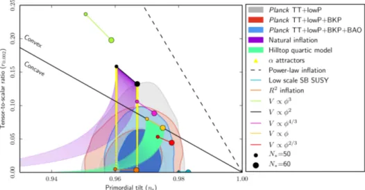
1.1 Marginalized joint 68 % and 95 % CL regions for nsand r at the pivot scale k∗ =
0.002Mpc−1 from Planck in combination with other data sets, compared to the theoretical predictions of selected inflationary models. . . 5 1.2 In this tree diagram we present the ways towards more elaborated inflationary
model building. . . 5 1.3 In the top-down motivation we build models in the low EFTs of string
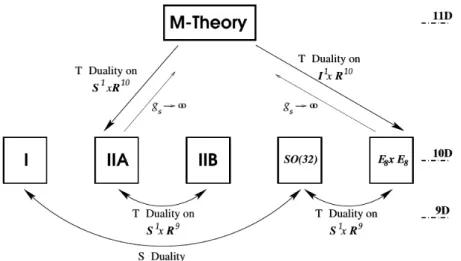
theory/M-theory which can be realized via compactifications on Calabi-Yau manifolds. In the bottom-up motivation we build models based on the physics beyond the SM of particle physics e.g., in GUTs and MSSM. . . 7 1.4 The various duality transformations that relate the superstring theories in nine and
ten dimensions. T-Duality inverts the radius R of the circle S1or the length of the finite interval I1, along which a single direction of the spacetime is compactified, i.e. R → l2
P/R. S-duality inverts the (dimensionless) string coupling constant
gs, gs → 1/gs, and is the analog of electric-magnetic duality (or strong-weak
coupling duality) in four- dimensional gauge theories. M-Theory originates as the strong coupling limit of either the Type IIA or E8× E8heterotic string theories. . 8
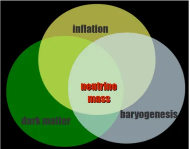
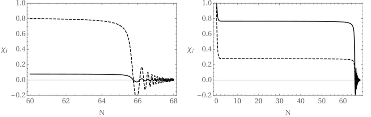
1.5 Inflation in particle physics motivated models such as GUTs and MSSM are par-ticularly interesting, when considering neutrino masses, DM and baryogenesis. Neutrinos are worthy elements beyond SM particle physics. . . 9 2.1 Left panel is the graphical representation of the numerical solutions of (2.37) and
(2.38) for χ1(N )(full line) and χ2(N )(dashed line) with θ≈
π
2 for the potentials
V1 = χ21 and V2= χ22. In the right panel, we depict the graphical representation
of the numerical solutions of (2.37) and (2.38) for χ1(N ) (full line) and χ2(N )
(dashed line) with θ =π
9. We have taken the initial conditions as χ1(0) = 2.1× √ 1 3 and χ2(0) = 2.1× √ 1 3. . . 21
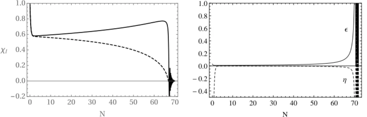
2.2 In the left panel we have the graphical representation of the numerical solutions of (2.37) and (2.38) for χ1(N )(full line) and χ2(N )(dashed line) with θ =
π
4 for the potentials V1 = χ21 and V2 = 2χ22. We have taken the initial conditions as
χ1(0) = 1.8× √ 1 3 and χ2(0) = 2.0× √ 1
3. In the right panel, and for the same
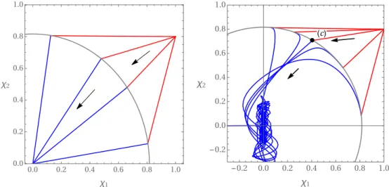
initial conditions, we have the graphical representation of the numerical solutions for ε (N ) (full line) and η (N ) (dashed line). . . . 22 2.3 This figure represents a set of trajectories evolving in the (χ1, χ2)space. These
trajectories are numerical solutions of (2.37) and (2.38) and correspond to a situa-tion where we choose V1= χ21and V2= χ22(left panel), as an illustrative example
only showing type I solution. All the fixed points are part of the arc of radius √
2/3in the (χ1, χ2) plane. In the right panel, we have an example, where we
have taken V1 = χ21 and V2 = χ42, showing type II solutions, except for the
tra-jectory going close to a fixed point with θ = π/3 (point C). In addition, in the right panel, we have an illustration of two 3-form fields damped oscillations by the end of inflation. The arrows, in the plots, indicate the direction of time in the trajectories. . . 23
of inflation (defined for ε = 1). We have taken V1 = V01(χ21+ bχ41) and V2 =
V02(χ22+ bχ 4
2)where V01 = 1, V02 = 0.93, b = −0.35 and with initial conditions
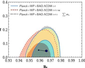
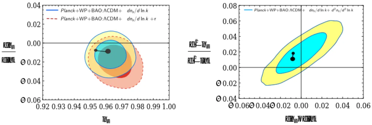
θ = π/4. . . 32 2.5 Graphical representation of the spectral index versus the tensor to scalar ratio, in
the background of Planck+WP+BAO data (left panel), for N = 60 number of e-folds before the end of inflation (large dot) and N = 50 (small dot). We have taken
V1= V01(χ21+ bχ41)and V2 = V20(χ22+ bχ42)where V01= 1, V20= 0.93, b =−0.35
for two 3-form. . . 33 2.6 Graphical representation of the running of the spectral index versus the spectral
index (left panel), and running of the running of the spectral index versus the running of the spectral index (right panel) in the background of Planck+WP+BAO data for N = 60 number of e-folds before the end of inflation (large dot) and
N = 50 (small dot). We have taken V1 = V01(χ21+ bχ41)and V2 = V20(χ22+ bχ42)
where V01= 1, V20= 0.93, b =−0.35 for two 3-form. This figure was also obtained
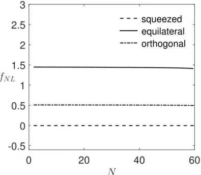
by taking the initial condition θ = π/4. . . . 34 2.7 In this plot we depict fNL against N for squeezed (k2≪ k1= k3) equilateral
(k1= k2= k3)and orthogonal (k1= 2k2= 2k3)configurations. We have
consid-ered the potentials V1 = V01
( χ2 1+ b1χ41 ) and V2 = V20 ( χ2 2+ b2χ42 ) with V01 =
1, V20= 0.93, b1,2=−0.35 and taken the initial conditions χ1(0)≈ 0.5763, χ2(0)≈
0.5766, χ′1(0) =−0.000224, χ′2(0) = 0.00014. . . . 40 2.8 Graphical representation of the non-Gaussianity shape fNL(α, β). We have
con-sidered the potentials V1 = V01
( χ21+ b1χ41 ) and V2 = V20 ( χ22+ b2χ42 ) with V01=
1, V20= 0.93, b1,2=−0.35 and taken the initial conditions χ1(0)≈ 0.5763, χ2(0)≈
0.5766, χ′1(0) =−0.000224, χ′2(0) = 0.00014. . . . 41
3.1 Evolution of the scale factor according to (3.16) (left panel) and the Hubble pa-rameter H, according to (3.18) (right panel). . . . 46 3.2 In the left panel we depict tensor-to-scalar ratio vs. spectral index where in the
plot N varies from 50 to 60 (from left to right) and cD varies from 0.087 to 0.6 (from bottom to top). In the right panel we plot the ratio r/nt vs. sound speed
cDfor N = 60. . . . 48 3.3 Plots of spectral index nsvs. tensor-to-scalar ratio r (left) and the ratio r/ntvs.
sound speed cD (right) in the Galileon limit. In the left panel, we take N varying from 50 to 60 (from bottom to top). For the right panel we considered N = 60. . 49 3.4 Contour plots in the plane ( ˜m, cD)(with ˜min units of mP). Blue and orange regions
represent the space where ns= 0.968± 0.006 and 0.01 ≤ r ≤ 0.1, respectively. . 50
3.5 Plots of spectral index ns vs. tensor-to-scalar ratio r (left panel) and the ratio
r/nt vs. m˜ (with ˜m in units of mP) (right panel) in the DBIG model. In the
left panel we take cD = 0.98 and 0.3 ≤ ˜m/mP ≤ 0.72 (red), cD = 0.985 and
0.5 ≤ ˜m/mP ≤ 1.25 (black), cD = 0.99 and 0.5 ≤ ˜m/mP ≤ 1.25 (blue). In the
plotted curves ˜mincreases as r decreases. In the right panel, the plotted curves correspond to cD= 0.98(red), cD= 0.985(black) and cD= 0.99(blue). . . 51 3.6 Plots of the mass squared of the inflaton field (left panel) and the non-Gaussian
parameter fNLeq (right panel) as a function of ˜m (with ˜min units of mP). In this
plot 0.22≤ α ≤ 0.32 for 0.5 ≤ ˜m≤ 1.25. We take cD = 0.985to build the plots, hence the depicted behaviour corresponds to the black line in Fig. 3.5. . . 52
represent the 68% and 95% CL for the spectral index ns, respectively. Black lines
represent contours for different values of the tensor-to-scalar ratio, as indicated. In the bottom panel, the blue region depicts the 95% CL for the spectral index ns.
We use cD = 0.980. . . . 54 3.8 In this plot, we depict the non-Gaussian parameter fNLequias a function of ˜m(with
˜
min units of mP). We take cD = 0.98and εf ∼ 10−4 (Blue line) and εf ∼ 10−6
(Green line). In this plot 0.326≤ α ≤ 0.33 for 1 ≤ ˜m≤ 20. . . 55
3.9 Predictions of the DBIG model for N = 60 along with the Planck TT+lowP+BKP+BAO constraints on the space (ns, r)at the 68% and 95% CL. The black line represents
the case with constant sound speed and warp factor (cD = 0.985, 1 ≤ ˜m/mP ≤
1.25). Different model predictions for a constant sound speed and varying warp factor are plotted in red (cD = 0.985, ˜m = 15mP and 5.1 ≤ 104εf ≤ 8.5), blue
(cD = 0.98, ˜m = 15mP and 1.5≤ 104εf ≤ 2.6) and green (cD = 0.98, ˜m = 13mP
and 0.07≤ 104ε
f≤ 0.11). . . 55
3.10 Evolution of the scale factor a(t), according to (3.40), for ¯λ1, ˙H > 0(left panel),
for ¯λ1> 0, ˙H < 0(central panel) and for ¯λ1, ˙H < 0(right panel). For simplicity
we take κ = 1. . . . 57 4.1 In the left panel we plot the potential VE
( ˜
ϕ
)
for values of ˜β = 10−5, 10−6 and ˜
α = 1. In the right panel, we depict the corresponding minimum of the potential around ˜ϕ≈ 0. . . 72
5.1 Parametric plot of spectral index (ns)verses tensor scalar ratio (r). We have
con-sidered 60 number of efoldings with n = 1 ,−0.03 < β < −0.001 (or equivalently 0.166≲ α ≲ 0.17). . . 80 5.2 The left panel is the graphical presentation of the local shape of the
poten-tial verses scalar field during inflation. The right panel depicts the parameter
εverses N . We have taken β =−0.001 (or equivalently α = 0.167) for both plots. 81 5.3 In both plots orange shaded region corresponds to the constraint 0.962 < ns <
0.974. The blue shaded region in the left panel is for large field ∆ϕ > 1 whereas in the right panel is for small field ∆ϕ < 1. We have considered N = 60. . . . 82 5.4 Parametric plots of spectral index (ns)verses tensor scalar ratio (r) (left panel),
αverses the ratio of tensor scalar ratio and tensor tilt (right panel). In these plots the blue line denote predictions for small field inflation for which we take
β ∼ −0.002 and 0 < n < 10. In this case r → 0 as n → 0 (equivalently α → 0).
The black line denote predictions for large field inflation for which β∼ −0.01 and 2 < n < 10. In this case r≳ O(10−3). We have considered N = 60. . . . 83 5.5 Plot of tensor scalar ratio (r) verses α. Here we have taken β ∼ −0.002 and
0 < n < 10. This plot is for N = 60. . . . 83 5.6 In this figure we depict the ratio of the square of masses to the square of Hubble
parameter H2. The red line indicates for ImΦ and the blue line is for S. We have
taken n = 1, α = 0.167, g = 0.5 and γ = 0.2. . . . 84 6.1 The dashed line denotes the CW potential in SV model. The full line indicates
the shape of the potential obtained in (6.36) which comes from the insertion of conformal symmetry in SU(5). When φ≫ µ the above VEV branch of the potential approaches the plateau of Starobinsky model. . . 97
the e-folding number. The solid blue line indicates the evolution of canonically normalized field φ, whereas the dotted blue line is for the original field ϕ. In the right panel we plot the corresponding slow-roll parameter ε verses N . Inflation ends when ε = 1. For both plots we have taken µ = 1.12mP. . . 99
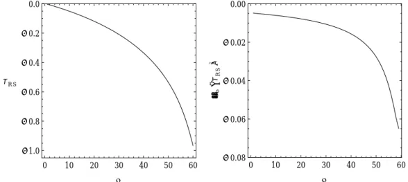
6.3 In this plot we depict the reheating temperatures TR Vs. mφ for the values of
2.1 Summary of some type I solutions critical points and their properties. . . 21 3.1 Inflationary observables in various limits of DBIG inflation. . . 54 6.1 Inflationary predictions of the AV branch solutions for different parameter values. 99
ΛCDM Λcold dark matter
AdS/dS (Anti-) de Sitter
CAM Cosmological attractor models
CMB Cosmic Microwave Background
CW Coleman-Weinberg
DBIG Dirac-Born-Infeld Galileon
EFT Effective field theory
GL Goncharov-Linde
GS Gong and Sasaki
GUTs Grand unified theories
FLRW Friedmann-Lemaître-Robertson-Walker
LSS Large Scale Structure
RHNs Right handed neutrinos
SBCS Spontaneous breaking of conformal symmetry
SM Standard model
SFT String field theory
SUSY Supersymmetry
SUGRA Supergravity
SV Shafi-Vilenkin
1
Introduction
It took less than an hour to make the atoms, a few hundred million years to make the stars and planets, but five billion years to make man
– George Gamow, The creation of the Universe
The classical Big Bang cosmology scenario proposed by G. Gamow in 1946 [1], was supported by the first detection of Cosmic Microwave Background (CMB) reported by A. A. Penzias and R. W. Wilson in 1965 [2]. However, such setting suffered from serious difficulties that became known as horizon and flatness problems [3]. Moreover, the development of Grand Unified Theories (GUTs) in the late 70’s [4] predicting the unification of strong, electromagnetic and weak in-teractions at the energy scales∼ 1016 GeV, revealed the possible over production of magnetic
monopoles, in the early Universe, which was known as monopole problem [5]. These prob-lems could be solved by means of an accelerated (near de Sitter) expansion of the Universe, as proposed by A. A. Starobinsky and A. H. Guth [6, 7], which is designated as the theory of
cosmological inflation. This theory was subsequently improved by the proposals of, A. D. Linde
[8, 9], A. Albrecht and P. J. Steinhardt [10], which were known as chaotic inflationary scenario and new inflationary scenario, respectively. Afterwards, V. F. Mukhanov, G. V. Chibisov and S. W. Hawking [11, 12] provided an explanation for the Large Scale Structure (LSS) formation seeded by primordial quantum fluctuations, which made the theory of inflation observationally attractive. In order to have an adequate particle production at the end of inflation, a reheating process [13, 14] is expected, constituting an intermediate stage in the evolution of the Uni-verse, subsequently leading into a radiation dominated era and then a matter dominated era. Currently, the inflationary paradigm has been widely accepted and stands as an essential mech-anism abridging the epoch of quantum gravity, the theory of all fundamental interactions and elementary particles (i.e, physics near the Planck energy scale), to our present day understand-ing of particle physics. In summary, the theory of inflation combines features imported from particle physics, astrophysics and cosmology to border and connect to a theory of everything. Once the exponential expansion begins, the Universe rapidly becomes homogeneous, isotropic and spatially flat, which can be described by a Friedmann-Lemaître-Robertson-Walker (FLRW) metric. During the inflationary regime, the Universe scale factor a(t) (which is a function of cosmic time t) increases exponentially, leaving the Hubble parameter H = 1
a da
dt almost
con-stant [15]. This implies the comoving Hubble radius (aH)−1 to decrease during this period i.e.,
d dt
( 1
aH
)
< 0for the time t∗ < te, where t∗, te mark the beginning and the end of inflation,
respectively. To solve the horizon and flatness problems it is essential that the scale factor during inflation should increase at least N = 50− 60 number of e-foldings where N = ln
(
a(te)
a(t∗)
) [15].
The required inflationary dynamics can be retrieved either by modifying General Relativity or by the addition of hypothetical matter fields which means modifying either left hand or right hand side of the Einstein equations, given by
Rµν− 1 2gµνR = 1 m2 P Tµν, (1.1)
where we fix the unitsℏ = 1, c = 1, m2 P =
1
8πG with the value of reduced Planck mass mP =
2.43× 10¹⁸GeV. Here R
µν is the Ricci tensor, R is the Ricci scalar, Tµν is the energy-momentum
tensor and gµν is the spacetime metric tensor1. The scalar field responsible for inflation is
usually named as inflaton, when it is a hypothetical matter field or scalaron when it emerges from modified gravity. In this thesis, we are mainly interested in finding inflaton candidates. An adequate period of exponential expansion ending in a reheating epoch can be met when the so called slow-roll parameters ε, η satisfy the following conditions during inflation [16]
ε =− ˙ H H2 ≪ 1 , η = ˙ ε Hε ≪ 1 , (1.2)
where over dot indicates the differentiation with respect to t.
The temperature fluctuations in the CMB are caused by the primordial quantum fluctuations of the scalar degrees of freedom during inflation [15]. In other words, the source of inflationary expansion and LSS of the Universe can be traced back to the dynamics and nature of one or more scalars. Inflationary background fluctuations (primordial modes) are created quantum mechanically at subhorizon scales k ≫ aH, where k is the comoving wavenumber. The CMB temperature anisotropy and LSS can be explained by the evolution of those fluctuations on superhorizon scales k≪ aH.
The quantum fluctuations during inflation can depicted by the curvature perturbation ζ in the comoving gauge2. In the case of single field inflation, ζ gets conserved on superhorizon scales.
Therefore, the fluctuations are adiabatic and the power spectrum measured at the time of horizon exit k∼ aH, is related to the temperature anisotropies in the CMB [17, 18]. Whereas in the case of multifield inflation, ζ evolves on the superhorizon scales as it is additionally sourced by isocurvature modes. In this case ζ is computed either by using transfer functions or the so called δN formalism [19–23].
The key observables of inflationary scenarios are related to the two-point and higher order correlation functions of curvature perturbation (see Appendix. A.1 for a brief review). The two-point correlation function of ζ defines the scalar power spectrum which predicts the Gaussian distribution of density fluctuations. Inflationary expansion obeying conditions (1.2) predicts that the scalar power spectrum would departure from exact scale invariance. This is quantified by a parameter named scalar spectral index, or scalar tilt, nsthat should differ from unity.
The other prediction of inflationary theory is the primordial gravitational wave power spectra, that can be defined in a similar way to the scalar power spectrum as a two point correlation function of tensor modes. The ratio of tensor to scalar power spectrum r and the tensor tilt nt,
defined in a similar way as ns, are crucial to test any model of inflation against observations.
In the context of the recent results from Planck satellite in 2015 [24, 25] and the joint analysis of BICEP2/Keck Array and Planck (BKP) [26], the single field inflationary paradigm, emerges as
1Throughout the thesis, we set the metric signature (−, +, +, +), small Greek letters are the fully
covariant indexes.
2
The details of other gauge choices can read from [15]. Throughout this thesis we use the notation for curvature perturbation either ζ orR [15], bearing the fact that the curvature perturbation defined on uniform density hypersurfaces ζ and the comoving curvature perturbationR are nearly equal in the slow-roll inflation (see [15] for details).
adequate to generate the observed adiabatic, nearly scale invariant and the highly Gaussian density fluctuations imprinted as the CMB temperature anisotropies. Moreover, the data is very much consistent with ΛCDM model3 of the current Universe and the results also indicate that
we live in a spatially flat Universe [27].
The CMB observations from Planck 2015 [24], constrains the scalar spectral index and the tensor to scalar ratio as
ns= 0.968± 0.006 , r < 0.09 , (1.3)
with respect to Planck TT+lowP+WP at 95% confidence level4 (CL) which rules out scale invari-ance at more than 5σ [24]. Furthermore, the data suggests a small running of the spectral index
dns/d ln k = −0.003 ± 0.007, which is consistent with the prediction from single field models
of inflation [18]. So far, there is no significant detection of primordial tensor modes (from the value of r), which is crucial to fully confirm the inflationary paradigm. A concrete measure-ment of r relates to an observation of the so called B-mode polarization amplitude, which can only be caused by primordial tensor modes in the CMB radiation. Moreover, the latest results suggest so far no evidence for a blue tilt of the gravitational wave power spectra i.e., nt > 0
from a very preliminary statistical analysis [24, 26]. The proposed post-Planck satellites CMBPol, COrE, Prism, LiteBIRD and many other ground based experiments such as Keck/BICEP3 [29–32] are expected to reach enough sensitivity to detect B-modes and establish if r∼ O(10−3). There is a considerable variety of different models of inflation that can be motivated theo-retically, but the degeneracy of the predictions from various models of inflation is an ongoing problem for cosmologists [33, 34]. One way to probe further the nature of the inflaton field is to study the statistics of the perturbations it produces beyond the two-point correlation func-tion [35–37], starting with the three-point funcfunc-tion. The latter is parametrized in Fourier space by the bipsectrum (defined in Appendix. A.1), a function of the amplitude of three wave vec-tors that sum to zero as a consequence of momentum conservation. The bispectrum of “local shape”, is a function of three wave numbers that peaks in the squeezed limit where two wave numbers are much larger than the third. The bispectrum of “equilateral shape” tends to zero in the squeezed limit, but peaks when all three wave numbers are similar in size. A third shape is often considered that peaks on folded triangles, where two wave numbers are approximately half of the third. Introducing three parameters floc
NL, f equi NL and f
ortho
NL , which parametrize the
overall amplitude of a local, equilateral and orthonormal shapes for the bispectrum, Planck 2015 data [25] informs us that
fNLloc= 0.8± 5.0 , f equi NL =−4 ± 43 , f ortho NL =−26 ± 21, (1.4) at 68% CL.
Any confirmation of non-Gaussianities in the CMB would be a significant information about the nature of the inflaton field [37]. For example, establishing through unequivocal observations and data analysis a local non-Gaussianity would rule out all the single field models of inflation [38].
3
Λstands for the cosmological constant and the CDM means the Cold Dark Matter.
4
Here TT+lowP+WP indicates the combined results of Planck’s angular power spectrum of tempera-ture fluctuations with low-l polarization (of CMB radiation) likelihood analysis and polarization data from Wilkinson microwave anisotropy Probe (WP) [28].
1.1
Standard scalar field inflation and Planck data
The simplest standard mechanism to set up inflationary expansion is conveyed by a (canonical) scalar field minimally coupled to Einstein gravity dictated by the following action
S = ∫ d4x√−g [ m2 P 2 R− 1 2∂µφ∂ µφ− V (φ) ] , (1.5) where g is the determinant of the metric gµν.
To sustain inflationary expansion long enough, the general ingredient has been that the potential
V (φ)needs to dominate over the kinetic term−1 2∂µφ∂
µφ, for which the inflaton is required to
be almost constant during inflation. This is achieved by the slow-roll approximation, which can be expressed in terms of potential slow-roll parameters5 as
εV ≡ m2P 2 V′(φ) V (φ) ≪ 1 , ηV = m 2 P V′′(φ) V (φ) ≪ 1 , (1.6)
where ‘a prime’ denotes differentiation with respect to the argument φ. The scalar spectral index nsand the tensor to scalar ratio r read as [15]
ns= 1− 6ε∗V + 2ηV∗ , r = 16ε∗V , (1.7)
where ”∗” denotes the quantities evaluated at the horizon exit. The energy scale of inflation can be estimated as Minf≡ V
(1/4)
∗ ≃ MGUTr(1/4)and the range of values that the field can take
during inflation can be determined by the Lyth bound [39–41]. In Appendix. A.2, we summarize the observational tests of standard single field inflation.
The constrains from Planck and BICEP2/Keck array data [24] rule out several potentials for a standard scalar field (see Fig. 1.1), nevertheless the flat ones of the following form
V ∼ ( 1− e− √ 2/3Bφ)2n , (1.8)
became successful candidates for the description of inflation and appeared in various scenarios [33, 34, 42]. The parameter B, in the above potential, can lead to any value of r < 0.09 with a fixed value for ns, namely
ns= 1−
2
N , r =
12B
N2 . (1.9)
We note that the potentials of the form in (1.8) cannot be easily justified field theoretically in the standard scalar description.
In the case6 of B = 1 the potential is the same as the one in the Einstein frame description of
Starobinsky’s R + R2inflation [6, 43] and also in the Higgs inflation with a non-minimal coupling
[44]. Although, these two models occupy a privileged position in the ns−r plane of Planck 2015,
it is still not possible to distinguish these two models observationally. The difference between these models is greatly expected to be found at the reheating phase [45], whose observational reach is uncertain in the near future [46].
5These are related to the general slow-roll parameters in (1.2) as ε≈ ε
V, η≈ 4εV − 2ηV [15].
6
The potentials with B̸= 1 requires more complicated realization of inflation in a fundamental theory which we will discuss later in Sec. 1.3.
Figure 1.1: Marginalized joint 68 % and 95 % CL regions for nsand r at the pivot scale k∗= 0.002Mpc−1 from Planck in combination with other data sets, compared to the theoretical predictions of selected
inflationary models.
1.2
Beyond standard scalar inflation?
Minimal canonical scalar (standard) Complexity Non-minimal canonical scalar Minimal Non-canonical scalar Non-minimal Non-canonical scalar Generalized scalar-tensor (or) Horndeski theories
Figure 1.2: In this tree diagram we present the ways towards more elaborated inflationary model building.
The standard scalar field action can be extended (cf. Fig. 1.2) either with a non-minimal cou-pling to gravity (e.g., Higgs inflation [44]) or with a non-canonical kinetic term7. Furthermore,
a general scalar-tensor theory was written and is known as Horndeski theory [48], which was shown to be equivalent to generalized Galileon model (G-inflation) [49]. The details about the G-inflationary action and calculations of perturbation spectra are presented in Appendix. A.3.
7
In general, we can also add additional matter fields to play crucial role along with the inflaton e.g., in the case of Warm inflation, radiation plays crucial role [47]
The standard single field models predicts very much a Gaussian landscape, where any small non-Gaussianities are suppressed by the slow-roll parameters [35], whereas the non-canonical and multified models predict detectable levels of non-Gaussianities [50–53]. In Ref. [54] shapes of non-Gaussianities in the general scalar-tensor theories were worked out, however the specific predictions are model dependent.
1.3
Top-down vs bottom-up motivations
Inflationary models can be phenomenologically realized in top-down or bottom-up (cf. Fig. 1.3) motivations as described below.
1.3.1
Top-down: Inflation in string theory/supergravity
According to the present observations, the Hubble parameter during inflation can be as large as 1013−14GeV, suggesting the scale of inflation to be of the order of M
inf≳ 1015GeV. These energy
scales are acceptable in theories of gravity promising ultraviolet (UV) completion, such as string theory/M-theory and supergravity (SUGRA), hence argued to play a crucial role in inflation [55]. Therefore, during the last years there have been many attempts to understand the inflationary picture from the low energy effective field theories (EFTs) motivated from such fundamental approaches [42, 56–58]. The interest of studying such inflationary scenarios is that it gives the best framework to get some observational indication of these fundamental theories. There has been a plethora of inflationary models in the literature, based on several modifications of the matter or gravity sector inspired from string theory/SUGRA [33]. Given our ignorance on the relation between a UV complete theory and its low energy effective limit, there is a plenty of room to construct models [34, 57] and aim to falsify them against current and future CMB observations.
M-theory, believed to explain all fundamental interactions including gravity, that describes the physics near Planck energy scale, is defined in a 11 Dimensional (11D) spacetime and claims to unify all five versions of superstring theories8 [60, 61], as presented in Fig. 1.4 (taken from
Ref. [62]). The idea of building inflationary models within string theory allows to test possible 4D low energy EFTs of these five superstring theories. In principle, to obtain a low energy limit of any version of superstring theory into 4D, we need to compactify six extra dimensions on small internal manifold such as Calabi-Yau9 and we thus are generically left with many possibilities
to construct 4D EFTs [66, 67]. Studying inflation in these theories is therefore most pertinent [61, 68, 69].
Broadly, inflationary scenarios in string theory can be divided into two categories: 1. Open string inflation (e.g., Brane/Anti-brane inflation) ;
2. Closed string inflation (e.g., Moduli inflation) .
A detailed review and recent observational status (with respect to Planck 2015 data) of several of these inflationary scenarios, driven by closed and open string fields, can be found in [33, 57,
8Which are related by T-, S- dualities [59–61] 9
Moreover, these compactifications have to be well stabilized to accommodate sufficient conditions for inflation to happen in the resultant EFT. For example, this was successfully prescribed in type IIB string theory through KKLT and KKLMMT scenarios [63–65].
String theory/M-Theory Inflation Standard Model of Particle Physics Low energy limit Beyond SM ~ 1016 GeV ~ 1018 GeV ~100 GeV Calabi-Yau
Figure 1.3: In the top-down motivation we build models in the low EFTs of string theory/M-theory which can be realized via compactifications on Calabi-Yau manifolds. In the bottom-up motivation we build
models based on the physics beyond the SM of particle physics e.g., in GUTs and MSSM.
58, 70]. Inflation in string theory contains several types of scalar field terms (e.g., Dirac-Born-Infeld (DBI) inflation where the scalar field is non-canonical), with fundamentally motivated choices of potentials, which can be tested by inflationary observables. With more precise CMB data, in the future we may aim to establish the role of string theory in inflationary dynamics, and help to fulfill our understanding of a fundamental theory [71].
Supergravity (SUGRA) is a gauge theory that is an extension of General relativity where we impose a local (gauged) supersymmetry (SUSY) and most SUGRA settings constitute a low energy limit of superstring theory. There are several versions of SUGRA, characterized by the number of massless gravitinosN = 1, .., 8. In particular, D = 4, N = 1 SUGRA could be an intermediate step between superstring theory and the supersymmetric standard model of particle physics that we hope to observe at low energies [72–75]. Therefore, it is realistic to construct EFT of inflation in D = 4,N = 1 SUGRA from high scale SUSY breaking10. Several inflationary models
in the past have been constructed in N = 1 SUGRA and they stand out to be an interesting possibility in regard of Planck data [42, 77]. Moreover, inflation in SUGRA has the interesting feature of predicting particle DM candidates (e.g., massive gravitino11) [78]. Inflation in SUGRA
is usually described by the Kähler potential as well as superpotentials, which depend on the chiral superfields [72, 79]. A brief discussion of SUSY breaking mechanisms for different SUGRA inflationary scenarios can be found in [80].
As mentioned previously, the observational data provided a special stimulus to study inflation with flat potentials of the form (1.8), which became successful candidates [33, 34, 42]. Such potentials are so far shown to occur in the low energy effective models of string theory/SUGRA
10If SUSY is not found in the current collider experiments, then high scale SUSY breaking is a natural
expectation in a UV complete theory; inflation can thus be a testing ground for high scale SUSY breaking [76].
11
Gravitino is the supersymmetric partner of graviton with spin= 3
2 which can gain mass due to SUSY
Figure 1.4: The various duality transformations that relate the superstring theories in nine and ten dimensions. T-Duality inverts the radius R of the circle S1 or the length of the finite interval I1, along
which a single direction of the spacetime is compactified, i.e. R→ l2
P/R. S-duality inverts the
(dimensionless) string coupling constant gs, gs→ 1/gs, and is the analog of electric-magnetic duality (or
strong-weak coupling duality) in four- dimensional gauge theories. M-Theory originates as the strong coupling limit of either the Type IIA or E8× E8 heterotic string theories.
and modified gravity [81–87]. A generic structure of Kähler potentials in SUGRA suitable for inflation and a possible connection to the open/closed string theory were studied in [88].
1.3.2
Bottom-up: Inflation and particle physics
Inflation has convincingly abridge cosmology with our present knowledge of particle physics, through the process of reheating: the scalar mode that drives expansion settles to a (true) vacuum, leading to particle production through a mechanism that depends on how the inflaton oscillates when it reaches to the minimum of the potential [13, 14]. This has strongly motivated the construction of inflationary models within the standard model (SM) of particle physics and beyond. Therefore, in a bottom-up motivation, several particle physics models were proposed including Higgs inflation, within grand unified theories (GUT) [44, 89–91] and Minimally Super-symmetric extensions of SM (MSSM) [33]. The interesting feature of a bottom-up motivation is that these models can be tested outside the scope of CMB e.g., at collider experiments. In the particle physics context, SM Higgs inflation [44] is particularly interesting due to the fact that Higgs was the only scalar so far found at LHC [92]. Nevertheless, for Higgs to be a candidate for inflaton, it requires a large non-minimal coupling12. On the other hand, SM is known to be
incomplete due to the mass hierarchy problems e.g., the Higgs mass being very low (125 GeV) compared to GUT scale, plus nearly but not quite negligible neutrino masses (∼ 0.1eV). Further-more, observed matter anti-matter asymmetry and dark matter find no explanation within SM. In this regard, inflationary models beyond SM physics i.e., GUTs and MSSM, are quite natural to explore [95, 96] (see Fig. 1.5 which is taken from [97]). The main advantage of studying inflation in SM extension theories is that in these constructions it is more natural to accommo-date the reheating process after inflation and moreover, we can expand the observational tests
12
It was known that a scalar field with large non-minimal coupling gives rise to a R2 term considering
1-loop quantum corrections. Consequently, renormalization group (RG) analysis shows that Higgs inflation is less preferable compared to Starobinsky model [93, 94].
beyond CMB, something that is more difficult to achieve when we consider models in the string theory/SUGRA. However, on the other hand there is a hope that the GUTs and MSSM can be UV completed in heterotic superstring theories [98–100].
Figure 1.5: Inflation in particle physics motivated models such as GUTs and MSSM are particularly interesting, when considering neutrino masses, DM and baryogenesis. Neutrinos are worthy elements
beyond SM particle physics.
1.4
Overview of the thesis
In this thesis, we study the following inflationary scenarios based on string/SUGRA and GUTs, which we show to be compatible with constraints from Planck data [24].
• Chapter 2: Multiple 3-form field inflation and non-Gaussianity
p-form fields13 are part of type IIA string theory [60, 61] where they generically appear as the gauge fields of SUSY multiplets. p−form fields are massless in the standard Calabi-Yau compactifications while in the low energy effective theories, p−form fields can gain mass via the Stückelberg mechanism [101, 102]. In the broader class of p−form inflation [103, 104], 3-forms are realized to be viable alternative to scalar field inflation [105, 106]. Moreover, in D = 4, 3−form fields are relevant and they have been studied especially in
N = 1 SUSY theories with quadratic potentials14[107–109]. In this chapter, we generalize
the single 3-form inflation with multiple 3-form fields and find suitable (phenomenological) choice of potentials compatible with observations. We also compute the corresponding generation of non-Gaussianities in this model.
• Chapter 3: DBI Galileon inflation
D-branes are fundamental objects in string theory to which open strings are attached, satisfying Dirichlet boundary condition [60]. Inflationary scenarios involving D-branes are associated with the motion of the branes in internal dimensions. These models are promis-ing ones in strpromis-ing cosmology [61]. In particular, the Dirac-Born-Infeld (DBI) inflation has
13A covariant tensor of rank p, which is anti-symmetric under exchange of any pair of indices is called p-form.
14
gained substantial attention in recent years [110–118] via low energy effective versions of type IIB string theory andN = 1 SUGRA [58, 67, 119, 120]. In this chapter we study a well motivated extension of this model, known as DBI Galileon inflation, and show that it enables a wider compatibility with Planck data.
• Chapter 4: Effective models of inflation from an SFT inspired framework
Assuming stringy energy scales are relevant at inflation, the field theory of interacting strings i.e., string field theory (SFT) would perhaps be crucial to be accounted [121, 122]. There were early attempts of considering inflation in SFT studied with p−adic strings [123, 124]. In this chapter, admitting non-locality being the distinct feature of SFT which is associated with how the string fields interact (see Appendix. D for details), we intro-duce a framework motivated from open-closed string field theory coupling; the open string tachyon condensation ends up in an inflationary (in general a constant curvature) back-ground with a stabilized dilaton field. We demonstrate that this configuration leads to interesting effective and viable models of inflation.
• Chapter 5: Non-slow-roll dynamics in α−attractors
The so-called α−attractor models are very successful with Planck data, predicting any value of r < 0.09 with ns = 0.968for N = 60. The predictions of this model are strongly
connected to the mathematical features of the inflaton’s kinetic term [125]. These models were first proposed inN = 1 SUGRA in the context of superconformal symmetries [83]. In this chapter, we study the model in non-slow-roll (or) Hamilton-Jacobi formalism [126, 127], which is different from standard slow-roll approximation discussed in Sec. 1.1. • Chapter 6: Conformal GUT inflation
Coleman-Weinberg (CW) inflation proposed by Q. Shafi and A. Vilenkin [89, 90] was the first model of inflation proposed in the context of GUTs such as SU(5) and SO(10), where inflation is the result of GUT symmetry breaking. In this chapter, we generalize this model with conformal symmetry whose spontaneous symmetry breaking, in addition to the GUT symmetry, flattens the CW potential. As a result we obtain ns ∼ 0.96 − 0.967 and r ∼
0.003− 0.005 for 50 − 60 number of e-foldings. We compute the predictions for proton life time and get values above the current experimental bound [128]. We implement type I seesaw mechanism by coupling the inflaton field to the right handed neutrinos. We further study the reheating and baryogenesis in this model through non-thermal leptogenesis.
2
Multiple 3-form field inflation and non-Gaussianity
One of the basic things about a string theory is that it can vibrate in different shapes or forms, which gives music its beauty
– Edward Witten
Considered as a suitable alternative to the conventional scalar field, single 3-form inflation has been introduced and studied in Ref. [105, 106, 129, 130]. In [129] a suitable choice of the po-tential for the 3−form has been proposed in order to avoid ghosts and Laplacian instabilities; the authors have shown that potentials showing a quadratic dominance, in the small field limit, would introduce sufficient oscillations for reheating [129] and would be free of ghost instabili-ties. In [130], it was shown that single 3-form field is dual to a non-canonical scalar field whose kinetic term can be determined from the form of 3-form potential. Therefore, similar to the non-canonical scalar field 3-form field perturbations propagate with a sound speed 0 < cs ≲ 1
which produces effects into inflationary observables. In [130], single 3-form inflation was shown to be consistent with ns= 0.97for power law and exponential potentials and the corresponding
generation of large non-Gaussianities were studied for small values of sound speed.
In this chapter, we extend the single 3-form framework to N 3-forms and explore their sub-sequent inflationary dynamics. We particularly focus on two 3-forms scenario for which we compute the power spectra relevant for the observations at CMB. More concretely, we obtain the inflationary observables for suitable choice of potentials and aim to falsify the two 3-forms inflationary scenario. In this regard, this chapter is divided into two main sections. The first sec-tion is dedicated to study of the different type of inflasec-tionary scenarios driven by two 3-forms. We study the evolution of curvature perturbation on superhorizon scales (csk≪ aH) effected
by the dynamics of isocurvature perturbations. For this we compute the transfer functions that measure the sourcing of isocurvature modes to the curvature modes on superhorizon scales. We obtain the observables such as scalar spectral tilt and its running, tensor to scalar ratio. In the second section, we compute the non-Gaussianities generated by two 3-forms dynamics. We compute the bispectrum using the fact that 3-form fields are dual to a non-canonical scalar fields. We compute reduced bispectrum fNLon superhorizon scales using our prescription of δN
formalism applied to the 3-forms. We predict the values of fNL parameter in different limits of
3-momenta for the same choice of potentials studied in the first section. Finally, in Sec. 2.2.3 we confirm, in particular, that two 3-forms inflationary scenario is compatible with current observational constraints.
2.1
Inflation with multiple 3-forms and primordial power
spec-trum
This section is organized as follows. In Sec. 2.1.1 we identify basic features ofN 3-forms slow-roll solutions, which can be classified into two types. We also discuss how the inflaton mass can be brought to lower energy scales, for large values ofN. In Sec. 2.1.2 we examine the possible inflationary solutions, when two 3-forms are present. There are two classes; solutions not able to generate isocurvature perturbations (type I); and solutions with inducing isocurvature effects (type II). We show that, using a dynamical system analysis1, the type I solutions does not bring
any new interesting features than single 3-form inflation [106, 129]. Type II case, however, characterizes a new behaviour, through curved trajectories in field space. Moreover, type II inflation is clearly dominated by the gravity mediated coupling term which appears in the equa-tions of motion. We present and discuss type II soluequa-tions for several classes of potentials, which are free from ghost instabilities [129] and show evidence of a consistent oscillatory behavior at the end of the two 3-forms driven inflation period. In addition, we calculate the speed of sound,
c2
s, of adiabatic perturbations for two 3-forms and show it has significant variations during
in-flation for type II solutions. Therefore, our major objective in this chapter is to understand and explore the cosmological consequences of type II solutions. In Sec. 2.1.3 we discussed adiabatic and entropy perturbations for two 3-form fields, using a dualized action [130, 131]. We distin-guish, type I and type II solutions with respect to isocurvature perturbations and calculate the power spectrum expression [18]. In Sec. 2.1.4 we present how our inflationary setting can fit the tensor to scalar ratio, spectral index and its running provided by the Planck data [132]. In this chapter, we follow the units mP= 1.
2.1.1
N 3-form fields model
In this section, we generalize the background equations associated to a single 3-form field, which has been studied in [105, 106, 129], toN 3-form fields. We take a flat FLRW cosmology, described with the metric
ds2=−dt2+ a2(t)dx2, (2.1) The general action for Einstein gravity andN 3-form fields is written as
S =− ∫ d4x√−g [ 1 2R− N ∑ I=1 ( 1 48F 2 I + V (A 2 I) )] , (2.2)
where A(I)βγδ is the Ith 3-form field and we have squared the quantities by contracting all the indices. The strength tensor of the 3-form is given by2
Fαβγδ(I) ≡ 4∇[αA (I)
βγδ], (2.3) 1Details presented in Appendix B.
2
Throughout this chapter, the Latin index I will be used to refer the number of the quantity (or the 3-form field) or the Ith quantity/field. The other Latin indices, which take the values i, j = 1, 2, 3, will indicate the three dimensional quantities; whereas the Greek indices will be used to denote four-dimensional quantities and they stand for µ, ν = 0, 1, 2, 3.
where anti-symmetrization is denoted by square brackets. As we have assumed a homogeneous and isotropic universe, the 3-form fields depend only on time and hence only the space like components will be dynamical, thus their non-zero components (for FLRW background) are given by
A(I)ijk= a3(t)εijkχI(t) ⇒ A2I = 6χ 2
I, (2.4)
where χI(t)is a comoving field associated to the Ith 3-form field and εijk is the standard three
dimensional Levi-Civita symbol. Also note that by introducing the more convenient field χI(t),
which is related to the corresponding 3-form field by the above relation, we have, subsequently, the following system of equations of motion forN 3-form fields
¨
χI+ 3H ˙χI+ 3 ˙HχI+ V,χI = 0 , (2.5)
where V,χI ≡
dV
dχI. For each value of I , each of the (2.5) are not independent: it is
straight-forward to see that a peculiar coupling is present through the Hubble parameter derivative, ˙H. This fact will play a crucial role, establishing different classes of inflationary behavior when more than one 3-from field is employed. In this setting, the gravitational sector equations are given by H2=1 3 { 1 2 N ∑ I=1 [ ( ˙χI+ 3HχI)2+ 2V (χI) ]} , ˙ H =−1 2 [ N ∑ I=1 χIV,χI ] . (2.6)
Therefore, the mentioned (gravity mediated) coupling between the severalN 3-form fields will act through the gravitational sector of the equations of motion. The total energy density and pressure of theN 3-form fields read
ρN= 1 2 N ∑ I=1 [ ( ˙χI+ 3HχI)2+ 2V (χI) ] , pN=−1 2 N ∑ I=1 [ ( ˙χI+ 3HχI)2+ 2V (χI)− 2χIV,χI ] . (2.7) We rewrite (2.5) as ¨ χI+ 3H ˙χI + V,χeffI = 0 , (2.8) where V,χeffI ≡ 3 ˙HχI+ V,χI = V,χI [ 1−3 2χ 2 I ] −3 2χI N ∑ J =1 I̸=J χIV,χI . (2.9)
terms of the variable
wI ≡
χ′I+ 3χ√ I
6 , (2.10)
where χ′I ≡ dχI/dN in which the number of e-folds of inflationary expansion is N = ln a(t).
Thus, we get H2χ′′I + ( 3H2+ ˙H ) χ′I+ V,χeffI = 0 . (2.11) The Friedmann constraint is written as
H2= 1 3 V (χI) (1− w2), (2.12) where w2≡ N ∑ I=1 w2I.
Employing the dimensionless variables (2.10), the equations of motion (2.11) can be rewritten in the autonomous form as
χ′I = 3 (√ 2 3wI − χI ) wI′ = 3 2 V,χI V ( 1− w2) ( χIwI− √ 2 3 ) +3 2 ( 1− w2) 1 VwI N ∑ J =1 I̸=J χJV,χJ, (2.13)
In the whole chapter, we study the sum separable potentials of the form
V =∑
I
VI(χI) . (2.14)
2.1.1.1 Dual action forN 3-forms
In general, any p-form in D dimensions has a dual of (D−p)−form [103, 130]. In our case 3-form field (A) and its field tensor four-form (F ) are dual to a vector and a scalar field respectively which can be expressed as [130]
Aµνρ= εαµνρBα, Fµνρσ=−εµνρσϕ , (2.15)
where εµνρσ is an antisymmetric tensor.
The corresponding action for the scalar field dual representation of theN 3-forms is [130, 133]
S =− ∫ d4x√−g [ 1 2R + P (X, ϕI) ] , (2.16) where P (X, ϕI) = N ∑ I=1 ( χIVI,χI− V (χI)− ϕ2 I 2 ) , (2.17) with X =−12GIJ(ϕ) ∂ µϕI∂µϕJ.
The dual fields are related to the 3-forms through the following relation [130, 133] XI =− 1 2∂µϕI∂ µϕ I = 1 2V 2 ,χI. (2.18)
For a background unperturbed FLRW cosmology, we can use the dualities defined in (2.18) to write the following relation between a 3-form field and its dual scalar field
ϕI = ˙χI+ 3HχI. (2.19)
Using the above relations, in the Lagrangian (2.17) we can identify the kinetic term to be
K(XI) = N
∑
I=1
(χIV,χI− V (χI)) . (2.20)
Since this kinetic term is only a function of χI and not of ϕI, this means that the field metric
is GIJ(ϕJ) = 1. Therefore, we have X =
∑
XI. The 3-from fields present on the right-hand
side of (2.17) should be viewed as functions of the kinetic terms XI though the inverse of the
relation (2.18).
Following the above relations we compute here the following quantities which we use later in our study P,X ≡ ∑ I P,χI= ∑ I P,χI ( ∂χI ∂XI ) =∑ I χI VχI . (2.21) And similarly P,XIXI = 1 V,χIχIV 2 ,χI − χI V3 ,χI . (2.22) P,XIXIXI = − V,χIχIχI V3 ,χIχIV 2 ,χI + 3χI V5 ,χI − 3 V4 ,χIV,χIχI . (2.23) P,I = −ϕI =− √ 6HwI. (2.24)
Considering the large amount of non-canonical scalar fields studies in cosmology, it might be tempting to think that given a 3-form theory the best way to proceed would be to simply pass to the dual scalar field theory and work solely with scalar field quantities. However, starting from a set of massive 3-form fields makes the task of analytically writing the dual scalar field theory very difficult, except for very particular potentials [130]. This can be seen by noting but the technical difficulty found when one tries to invert (2.18). Yet, in a similar manner to that advocated in Ref. [130] for the single field case, we will see that we can still make use of the dual theory indirectly.
2.1.1.2 Initial conditions and slow-roll inflation
Analogous to the scalar field [134] as well as single 3-form [105, 129] inflationary models, the so-called slow-roll parameters are taken as ε≡ − ˙H/H2=−d ln H/dN and η ≡ ε′/ε−2ε, which,
for our model, are given by3 3Equivalently solely in terms of χ
I and wI, η = ∑N I=13 (√ 2 3wI−χI )
(V,χI+V,χI χIχI)
∑N