✡ ✪ # ✱ ✑✑✑ ✟✟ ❡
❡ ❡ ❅
❅❅ ❧
❧ ❧ ◗
◗◗ ❍ ❍, , , ❳❳ ❳ ❤❤ ❤ ❤
✭ ✭ ✭
✭✏✟✏
IFT
Instituto de Física TeóricaUniversidade Estadual Paulista
DISSERTATION IFT–D.009/14
Application of open string field theory to the inflationary scenario
Guilherme Franzmann
Orientador Nathan Jacob Berkovits
merecer a consideração de críticos honestos e suportar a traição de falsos amigos; apreciar a beleza, encontrar o melhor nos outros; deixar o mundo um pouco melhor, seja por uma saudável criança, um canteiro de jardim ou uma redimida condição social; saber que ao menos uma vida respirou mais fácil porque você viveu. Isso é ter tido sucesso.” - Ralph Waldo Emerson
"Bem-aventurados são aqueles que promovem o auto-conhecimento, que buscam entender o sentido de suas próprias vidas. Felizes são aqueles que entendem que não fazem mal ao próximo, não por causa de alguma
1. Introduction 9
2. String Field Theory 11
2.1. Chern-Simons Theory . . . 11
2.2. Generalization of Chern-Simons theory . . . 12
2.3. Open String Field Theory . . . 14
2.3.1. The classical string field . . . 14
2.4. Cubic String Field Theory Action. . . 15
2.5. Evaluation method . . . 17
3. The Tachyonic Potential 21 3.1. The gauge choice . . . 21
3.2. Level truncation scheme . . . 22
3.3. The potential . . . 23
4. Inflation: motivations, qualitative description and old approaches 27 4.1. Historical Context . . . 27
4.2. A simple analogy . . . 27
4.3. The initial-condition issues . . . 29
4.3.1. Homogeneity, isotropy (horizon) problem . . . 29
4.3.2. Flatness problem . . . 30
4.3.3. Initial perturbation problem. . . 30
4.4. Inflation: qualitative aspects . . . 30
4.5. The old and new scenarios . . . 31
4.5.1. The old inflation . . . 31
4.5.2. The new inflation. . . 33
5. The chaotic inflation 35 5.1. Why chaotic? . . . 35
5.2. Slow-roll limit . . . 35
5.3. Slow-roll parameters . . . 37
5.3.1. Examples . . . 38
5.4. General picture in conformal diagrams . . . 41
5.5. The tachyonic potential . . . 43
5.5.1. A naive analysis . . . 43
6. Conclusion 47 A. Elements of Bosonic Open String Theory 49 A.1. String Action in the conformal gauge . . . 49
A.2. Operator Product Expansion (OPE) . . . 52
A.4. Mode Expansion . . . 54
A.4.1. Scalar fieldXµ . . . 55
A.4.2. bcfields . . . 56
A.5. Vertex Operators . . . 57
A.6. Tree-level Amplitudes . . . 57
B. BRST Quantization 59 B.1. The String Spectrum . . . 59
B.1.1. BRST Quantization . . . 60
B.2. BRST quantization of the string . . . 62
C. Calculations from Chapter 3 63 D. Elements of General Relativity and Cosmology 67 D.1. Our Universe . . . 67
D.2. Kinematics: causal structure . . . 69
D.2.1. Conformal Time . . . 69
D.2.2. Particle Horizon . . . 69
D.2.3. Event Horizon . . . 69
D.2.4. Redshift . . . 70
D.3. Dynamics . . . 70
D.3.1. Energy, momentum and pressure . . . 70
D.3.2. Friedmann Equations . . . 71
D.3.3. General example . . . 72
É natural que ao chegarmos ao fim de uma etapa lembremos inúmeros momentos e pessoas que fizeram parte desta jornada. Então aqui coloco meu reconhecimento a todos que estiveram presentes na minha vida ao longo dos últimos dois anos, em particular, agradeço
Ao Nathan, por ter me aceitado como seu aluno, incentivado minha vontade de ir fazer doutorado no exterior e toda liberdade que tive enquanto seu aluno para administrar meus estudos.
Ao professor Matsas, por sua disposição em conversar comigo e pela ajuda com inúmeras cartas de recomendação.
Ao professor Nastase, a quem considero um amigo pela tamanha ajuda que ofereceu em diversos momentos na minha busca por opções de doutorado fora do país, pela ajuda com todas as cartas de recomendação e por acreditar em mim como estudante.
À Rosane e à Luzinete, que estiveram sempre dispostas em me ajudar, e a todos os alunos, com cuidado e preocupação maternais.
Ao Marco, por termos transcendido a relação professor-aluno ainda enquanto eu estava na gradu-ação, ter ouvido muitas vezes meus lamentos do mundo acadêmico, pela sua constante preocupação e, principalmente, por ter me inspirado não só como pesquisador e professor, mas também como pessoa em diversos aspectos.
À minha família, que independente de todos os contratempos e diferenças, no final das contas estava lá para me ajudar a segurar um pouco do peso do mundo.
Ao George, pela amizade ao longo dos últimos seis anos e diversas horas de conversas na nossa sacada de madrugada. Também por aguçar meu interesse gastronômico.
Ao Patrice, pela rápida identificação na forma de pensar e inúmeras discussões vigorosas sobre física e filosofia.
Ao Lucas, que com seu modo de pensar fez com que eu percebesse diversas limitações do meu horizonte.
Ao Ernany, pela sua amizade e seu jeito único de ser.
Ao Fagner, pelo seu jeito apaixonante de ver a vida e com quem pude aprender com nossas conversas.
Ao Renann, pelos diversos momentos que viemos a passar juntos já no final da jornada, sua disposição em me ajudar com minhas dúvidas e por ser um grande homem. Literalmente.
Ao Carlisson, essa figura direto do Maranhão, que sempre esbanja um sorriso no rosto e traz uma história de determinação que a todos deveria inspirar.
Ao Henrique, porque a nossa relação deveria definir o termo primo-irmão. E acho que isso resume tudo que poderia ser dito.
Ao Fernando, Paulo, Daniel, Pedro, Prieslei e Luan, que de diferentes formas e em diferentes momentos, tornaram a jornada mais leve.
À Clara, pela grande amizade que desenvolvemos e com quem pude me identificar de maneiras que ainda desconhecia.
String Theory
In string theory, the basic assumption is that all the elementary particles are vibrations of a very small elastic string, generating a unification between the different kinds of elementary particles. The fact that a string has some extension also succeeds in eliminating infinites which come up when point particles approach each other too closely in Quantum Field Theory (QFT). These two properties together provide a good indication that String Theory could provide the correct framework to study a quantum gravity theory.
There are several types of string theory, depending essentially if we are considering bosons, fermions or both of them and what are the boundary conditions, resulting in open or closed strings. In this thesis, we will be concerned with the open bosonic sector.
Although we consider string-like objects, string theory is perturbative as QFT, that means, it is a formalism for calculating scattering amplitudes as a perturbation series over a small coupling constant. However, when one starts studying the spectrum of the open bosonic sector, the physical spectrum contains a tachyonic mode, indicating that anon-perturbativetheory has to be developed.
String Field Theory
The most successful non-perturbative theory developed so far was first introduced by Witten [3]. In fact, making use of the bc ghosts introduced to fix the symmetries in the string action, which results in the presence of aBRST symmetry, it was possible to construct a parallel with the already known Chern-Simons theory in 3−dim, providing a covariant action for the bosonic open string field theory.
The construction, as we will see, is very elegant and based in very intuitive arguments, providing an algorithm to consider string interactions. Using this framework, it is possible to calculate the effective tachyonic potential of the open bosonic sector and analyze the tachyon condensation dynamics, that is, how the tachyon field decays and its implications.
Cosmology and Inflation
It was known in the 70′sthat the Standard Cosmological Model by that time had some problems, related with the initial-conditions of the universe. As a matter of fact, the large isotropy and homogeneity of the universe in the Cosmic Background Radiation (CMB) were an indication of an extremely fine-tunning in the very early universe, which seemed very unnatural.
Then, in the beginning of the80′s, some works [16,17,25] leading by Guth’s paper [15] proposed
Strings and Cosmology
At first sight, string theory and cosmology, inflation in particular, could be thought as too "far away" to be related. However, recent developments of both fields have brought they together, especially concerning the very beginning of the universe.
In fact, cosmology and strings could complement each other in several ways. On one side, cosmology stills lacks an underlying theory to address the initial singularity problem and the origin of inflation. On the other side, string theory has not yet been confronted with experiments and this could be a good opportunity for it.
One way to put all the things together is considering the decaying of the tachyonic mode, having its dynamics (its potential) calculated in the open string field theory framework, as a candidate for the inflationary scenario. This will be the ultimate objective here, even though we might have to consider several approximations in order to keep the problem as simple as possible so that it remains pedagogic.
Summary of the Thesis
In the second chapter we introduce briefly the Chern-Simons theory and explicit the relevant properties that will be important for the construction of the open string field action. Then, we follow Witten’s prescription and provide the method to evaluate the action.
The third chapter presents the calculation of the tachyonic potential at the very first approxi-mation (to be explained there). Some of the calculations are omitted, but they are developed in the appendices.
Inflation is introduced only in chapter 4 through a historical and qualitative description. We provide an easy analogy to understand the main problems that motivated the introduction of this scenario in the early universe cosmology.
Chapter 5 brings inflation to its modern approach, focusing only in the classical properties and its consequences. We treat some example models to demonstrate the slow-roll approximation and, finally, build the bridge between the tachyonic potential calculated in chapter 3 and the inflationary paradigm.
The first construction of a gauge invariant string field theory appeared in [1] where the BRST approach was used. Soon after, in [2] a gauge invariant string field theory was constructed using a single string field and when tried to extend it to a minimal gauge invariant system, a BRST structure was seen to emerge. Even though these references will not be used any longer, they give a hint of the important task BRST symmetry shall play from now on.
This chapter is intend to review the construction of a consistent String Field Theory for bosonic open strings. The strategy is to interpret the interactions in this framework as defining a non-commutative and associative algebra which will have its elements identified with the string field and its derivative with the BRST operator. This algebra is analogous to the Chern-Simons theory, so we start providing a brief description of it.
Our prior references will be [3,4,5,6] and others that will be cited when necessary.
2.1. Chern-Simons Theory
Let’s start by reviewing the Chern-Simons theory in 2 + 1−dimensions since the open string field
action is inspired on the nonabelian version of it. A good reference for the classical and quantum aspects of this gauge theory can be found in [31].
The Chern-Simons theory is a gauge theory in2+1-dimensions1developed by Witten [32]. It has very interesting theoretical properties and practical application in condensed matter phenomena. Its Lagrangian is
LCS=
κ
2ǫ
µνρA
µ∂νAρ−AµJµ (2.1)
whereAµis the gauge field in 2 + 1−dim andJµ is the matter current. Under the gauge
transfor-mation Aµ→Aµ+∂µΛ it transforms as
δLCS =
κ
2∂µ(Λǫ
µνρ∂
νAρ). (2.2)
Therefore, its action is gauge invariant if we can ignore boundary terms. The equation of motion is
κ
2ǫ
µνρF
νρ=Jµ, (2.3)
whereFνρ=∂νAρ−∂ρAν is the field strength. Note that ifJµ= 0,we have Fνρ= 0, which looks
pretty trivial when compared with Maxwell theory, because there even the source-free Lagrangian provides interesting properties, as the plane-wave solutions. There are several ways to make the Chern-Simons theory more interesting2 in
2 + 1-dim, as considering the nonabelian version below.
The nonabelian Chern-Simons is given by
LCS=κǫµνρtr
!
Aµ∂νAρ+
2
3AµAνAρ
"
, (2.4)
1
Actually, it is possible to construct a Chern-Simons gauge theory for all the odd dimensions. On the other hand, it is only in3−dim that it is quadratic in the gauge field.
2
where Aµ = AaµTa, Aaµ are the gauge fields and Ta are the generators of a gauge Lie algebra,
satisfying [Ta, Tb] = fabcTc; fabc are the structure constants of the algebra. A variation of δAµ
induces a variation in the Lagrangian,
δLCS =κǫµνρtr(δAµFνρ), (2.5)
where Fµν =∂µAν−∂νAµ+ [Aµ, Aν].The equation of motion has the same form as the abelian
case, but now the field strength has an additional term.
In order to connect the nonabelian Chern-Simons theory with the open string field action more directly, we shall rewrite it using differential forms. Then, its action is
S(A) = 1 2
ˆ
M
A∧dA+1 3
ˆ
M
A∧A∧A, (2.6)
where M is a 3−manifold andA =AaTa is a 1−form. The integral symbol also includes a trace
over the Lie-algebra generators. If we consider the following properties 1. dis nilpotent: d2ω = 0 for all differential formsω;
2. dis a derivation: d(ω∧η) =dω∧η+ (−1)|ω|ω∧dη,where|ω|is the degree ofω; 3. cyclic symmetry: ´
ω∧η = (−1)|ω||η|´ η∧ω; 4. Stoke’s theorem: ´
dω= 0;
5. ∧is associative,
then (2.6) is invariant under the gauge transformation
δA=dǫ+A∧ǫ−ǫ∧A, (2.7)
withǫbeing a 0−form.
All the above properties, the gauge transformation and the Chern-Simons action will have analogs in Witten’s open bosonic string field theory.
2.2. Generalization of Chern-Simons theory
We start by following the Witten’s proposal to formulate the field theory of open string [3]. Its starting point is quite axiomatic: let’s consider an associative non-commutative algebraB with the defining properties:
1. a Z2 grading, so that for every elementb∈B we have a degree3 (−1)kb which is±1;
2. a multiplication law ⋆ defined as such: for any two elements a, b ∈ B, the degree of the producta ⋆b is(−1)ka·(−1)kb;
3. a linear map Q: for any b∈B, Q(b)∈B which obeysQ(a ⋆ b) = (Q(a))⋆ b+ (−1)kaa ⋆ Q(b).
Besides, Q is odd under the grading, which means that the degree of Q(b) is −(−1)kb and
Q is nilpotent, i.e., Q2=0, giving Q(Q(b)) = 0 for allb ∈B. We will call this linear map a "derivation" of the algebra.
3
4. a linear map´: for any
b∈B, ´
b∈Cwhich obeys ´
a ⋆ b= (−1)kakb´ b ⋆ a,where(−1)kakb
is defined to be(−1)ifaand bare both odd and+1otherwise. We also require that for any
b∈B,´
Q(b) = 0.This map will be called "integration".4
Before we continue, let’s call some attention for the above axioms in order to preview where we will get soon. The elements of our algebra will be identified with the cohomology of the BRST operatorQB with ghost number 1.
The above axioms are enough to generalize the Chern-Simons gauge theory. Let’s consider a field A with kA = 1 (in the language of differential forms, this would means a 1-form) with the
following gauge invariance
δA=Q(ǫ) +A ⋆ǫ −ǫ ⋆ A, (2.8) where ǫ is an arbitrary element of B with kǫ = 0 (a 0-form in the differential forms framework).
Note thatB contains a subalgebraB0 of elements withkB0 = 0. We can now define a field strength to be
F =Q(A) +A ⋆A (2.9)
which transforms under gauge transformations as
δF =F ⋆ ǫ−ǫ ⋆ A. (2.10)
Now, we can imagine the most general action to be written for the field A which preserves the above gauge invariance. It turns out that this action is given by the Chern-Simons three-form action,
S =
ˆ !
A ⋆Q(A) +2
3A ⋆ A ⋆ A
"
. (2.11)
Note that we do not consider higher Chern-Simons forms because they will have their integrals vanishing in the bosonic open string field framework (due to the precise ghost number associated with the correlators). We could have also considered the term ´
F ⋆ F, however it is easy to show it is a topological invariant since its variation under an arbitrary variation ofA is zero. Since this action pretty much constitutes the essence of this thesis, let’s show that it is gauge invariant under (2.8):
S =
ˆ
(A ⋆Q(A) +2
3A ⋆ A ⋆ A) =
ˆ
(A ⋆F −1
3A ⋆ A ⋆ A)
δS =
ˆ
{δA ⋆ F +A ⋆ δF −1
3[δA ⋆ A ⋆ A+A ⋆ δA ⋆ A+A ⋆ A ⋆ δA]} =
ˆ
{[Q(ǫ) +A ⋆ǫ −ǫ ⋆ A]⋆ F +A ⋆(F ⋆ ǫ−ǫ ⋆ F)−1
3[Q(ǫ) +A ⋆ǫ −ǫ ⋆ A]⋆ A ⋆ A+ +A ⋆[Q(ǫ) +A ⋆ǫ −ǫ ⋆ A]−1
3A ⋆ A ⋆[Q(ǫ) +A ⋆ǫ −ǫ ⋆ A]} =
ˆ
{Q(ǫ)⋆ F + 3
# $% &
A ⋆ ǫ ⋆ F−ǫ ⋆ A ⋆ F +A ⋆ F ⋆ ǫ−
3
# $% & A ⋆ ǫ ⋆ F−1
3[Q(ǫ)⋆ A ⋆ A+A ⋆Q(ǫ)⋆ A+
+A ⋆ A ⋆ Q(ǫ)]−1 3[
1
# $% & A ⋆ ǫ ⋆ A ⋆ A+
2
# $% &
A ⋆ A ⋆ ǫ ⋆ A+A ⋆ A ⋆ A ⋆ ǫ] + 1
3[ǫ ⋆ A ⋆ A ⋆ A+ (2.12) +
1
# $% & A ⋆ ǫ ⋆ A ⋆ A+
2
# $% & A ⋆ A ⋆ ǫ ⋆ A]}.
4
The terms with the same number cancel each other. Now, using axiom 4, we see that ˆ
Q(ǫ)⋆ A ⋆ A = (−1)kAkQ(ǫ)⋆A
ˆ
A ⋆Q(ǫ)⋆ A=
ˆ
A ⋆Q(ǫ)⋆ A, sinceQ(ǫ)⋆ Ais even; ˆ
A ⋆ A ⋆ Q(ǫ) =
ˆ
Q(ǫ)⋆ A ⋆ A, sinceA ⋆Ais even; ˆ
A ⋆ F ⋆ ǫ =
ˆ
F ⋆ ǫ ⋆ A=
ˆ
ǫ ⋆ A ⋆ F, sinceF ⋆ ǫandFare even; ˆ
ǫ ⋆ A ⋆ A ⋆ A =
ˆ
A ⋆ A ⋆ A ⋆ ǫ, sinceA ⋆Aand A ⋆ A ⋆ ǫare even, so that (2.12) becomes
δS =
ˆ
{Q(ǫ)⋆ F −
4
# $% & ǫ ⋆ A ⋆ F +
4
# $% &
ǫ ⋆ A ⋆ F−Q(ǫ)⋆ A ⋆ A}
=
ˆ
{Q(ǫ)⋆ F −Q(ǫ)⋆ A ⋆ A}
=
ˆ
{Q(ǫ)⋆ Q(A) + 5
# $% & Q(ǫ)⋆ A ⋆ A−
5
# $% & Q(ǫ)⋆ A ⋆ A}
=
ˆ
Q(ǫ)⋆ Q(A) =
ˆ
Q[ǫ ⋆ Q(A)] = 0.
2.3. Open String Field Theory
The first mode of the bosonic open string theory spectrum is a tachyon, which is a scalar field with an unstable potential. It is possible that this potential could be used to create an inflationary scenario. However, in order to study this possibility it is necessary to know how the potential associate with this tachyonic mode looks like. To calculate the potential, we have to go beyond the first-quantized framework, which is onshell. Hence we need an off-shell formulation of string theory, which is calledstring field theory,so that it is possible to obtain the potential. It is worth to mention that there are other reasons for the study of the off-shell formalism, between them the attempt to prove the Sen’s conjectures [35] and find the correct vacuum of string theory.
This section will be based on [4,5,6]. 2.3.1. The classical string field
As it can be reviewed in the appendixA, the Hilbert spaceHof the open string theory is constructed acting with the creation operators αµ−n, b−m, c−l, where m, n, l > 0, and c0 on the vacuum |Ω% ≡c1|0%,defined by
αµn|Ω%= 0 n >0
bn|Ω%= 0 n≥0
cn|Ω%= 0 n >0
pµ|Ω% ∝αµ0|Ω%= 0. (2.13)
Note that regarding the state-operator mapping, it is expected that the vacuum of the theory should be mapped to the unit operator. This property is, indeed, satisfied by the state|0%=|0; 0%⊗b−1| ↓%.
that is equal to |Ω%. So, due to the weights of b and c, the unit operator in the vertex operator formalism is not mapped to the ghost vacuum in the state formalism. As one can check, |Ω% is
mapped toc(0). Then, we have
|0%∼I , |Ω%∼c(0). (2.14)
A generic state is given by αµ1
−n1. . . α
µi
−nib−m1. . . b−mjc−l1. . . c−lk|Ω%, (2.15)
wheren >0, m >0, l≥0andi, j, k are arbitrary positive integers. As a result, any state|Φ% ∈ H
can be expanded as
|Φ%= [ϕ(x) +Aµ(x)αµ−1+Bµν(x)αµ−1αν−1+. . .]c1|0% ≡Φ(z= 0)|0%. (2.16)
Note that the coefficients multiplying the operators depend on the center-of-mass coordinate x of the string. As you can imagine, we have infinitely many coefficient functions and they are identified
with the spacetime particle fields, that is why we call |Φ% string field. The corresponding vertex operator, Φ(0),has the same name.
The Hilbert space defined above is redundant. We have treated this problem in the appendixB
considering the BRST quantization procedure. Now that we have established some aspects of the string field language, we can rewrite the physical conditions in this framework. In order to do this, let’s consider the action below defined upon the ghost number+1 states5:
S0 =+Φ|QB|Φ%. (2.17)
Using the reality condition for the string field, Φ[Xµ(π−σ)] = Φ∗[Xµ(σ)],the equation of motion is
QB|Φ%= 0, (2.18)
equal to the physical condition (B.15). Besides, it is easy to see that (2.17) is invariant under the gauge transformation
δ|Φ%=QB|χ%, (2.19)
where |χ% has ghost number 0. This corresponds to the exact state defined in (B.18). From the above, we notice that an on-shell state, which is a solution to the equation of motion of S0, is
a physical state in string theory. In order to obtain the interacting field theory, we will have to include higher orders terms in Φusing the generalization we have exposed already in section 2.2.
2.4. Cubic String Field Theory Action
After studying the generalization of the Chern-Simons theory in section2.2, we can construct our string field theory action considering the same axioms we have seen already with the identification of the BRST operator, QB, as the nilpotent derivative operator and string fields as the elements
of the algebra B.
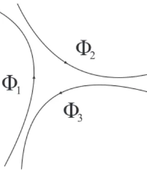
In order to understand better why this axiomatic approach makes sense to deal with open string field theory, we need to give a better look at the ⋆ product. First, let’s call attention to what is pointed out in [3]: we do not need to work with reparametrization invariant strings once we have imposed the conservation of the BRST charge, which is natural giving our identifications. Hence, the following construction will not be reparametrization invariant as we will be choosing a preferred point of the string, the mid-pointσ =π/2, remembering we are consideringσ∈[0,π].So, consider:
5
1. The ⋆−product will be associative if we interpret this operation as gluing two half-strings together as in Figure 2.1(a). We glue together the right hand piece of the string U, (π/2≤
σ ≤π), to the left hand piece of the string V, (0≤σ ≤π/2), remaining a string-like object composed by the left hand piece of U and right hand piece ofV. The resulting string state on U ⋆ V is the string fielda ⋆b;
2. Since we are considering a non-commutative operation,U ⋆ V andV ⋆ U are different. On the
other hand, the integration is defined as ´
a ⋆b = (−1)kakb´ b ⋆ a, i.e., it is "commutative"
ignoring the sign difference. That suggests us that the integration procedures glues the
remaining sides ofU andV. In(c),that would mean to sew together the left- and right-hand ends of the string U at its mid-point;
V
U W
U
V
0 0
ð/2
ð/2
ð
ð
U 0
ð/2
ð
U V
(a) (b) (d)
Figure 2.1.: (a) Gluing of two strings which have half of them coinciding in space-time. (b) Glu-ing three strGlu-ings shows qualitatively why associativity follows. (c) The integration operation sews together both halves of the string at its mid-point. (d) Multiplication followed by an integration, ´
(U ⋆ V).
Once the⋆-product and the integration operation is understood as above, we can consider to write the so called Witten vertex,
ˆ
Φ1⋆ ... ⋆Φn, (2.20)
whereΦi denotes a string field on theithstring Hilbert space. It is the3-string vertex that matters
for us, since it is for the cubic interaction term that we were able to generalize the gauge invariance. We represent this vertex below :
Ö
Ö
Ö
12
3
Figure 2.2.: 3-string vertex.
derivative operator, the algebraZ grading comes from the ghost number. It was already explained that the string field has ghost number+1. Besides, we consider that#gh(QB) = 1and#gh(⋆) = 0.
Now, we can understand why only the quadratic term and the 3−string vertex were considered
from the beginning. We know that the ghost number counts the number ofcghosts in the correlator minus the number of b ghosts. On the other hand, according to the Riemann-Roch theorem, we must have for each correlator
#cghost−#bghost= 3χ, (2.21)
where χis the Euler characteristic number for the surface considered. In the open string case, we are considering the disk6, which gives
χ= 1. Hence, the ghost number for each correlator is3,so that only the quadratic and cubic term were possible candidates from the beginning.
Finally, we can rewrite the action (2.11) for the open string interaction as
S =−
!ˆ
Φ⋆QBΦ+
2
3goΦ⋆Φ⋆Φ
"
, (2.22)
which is gauge invariant under
δΦ=QBǫ+go(Φ⋆ ǫ−ǫ ⋆Φ), (2.23)
where ǫ is a gauge parameter with ghost number 0 and go is the open string coupling constant.
Indeed, the action with which we will be working comes from redefining the string field asΦ→ αg′ oΦ
and changing the overall normalization such that S=− 1
g2
o
! 1
2α′ ˆ
Φ⋆QBΦ+
1 3
ˆ
Φ⋆Φ⋆Φ
"
. (2.24)
After considering the above construction, we can now state the correspondence between the nonabelian Chern-Simons theory in2 + 1- dim and the open string field theory in the table below:
Open String Field Theory Chern-Simons theory in differential forms
element string field differential k-form
degree (−1)#ghost (−1)k
multiplication ⋆−product ∧ (wedge product)
derivation QB exterior derivative d
integration ´ ´
on a k−dimensional manifold
2.5. Evaluation method
In the last section, we have justified why the relevant action to work the interactions in the string field theory framework is (2.24). However, we still do not know how to do calculations with it. Even though the quadratic term can be promptly associated with +Φ|QB|Φ%, the cubic term does
not have a ready translation.
There are more than one method to work out the interaction string field term. Here we will be considering a conformal field theory approach, in which conformal mappings and calculation of correlators in the disk will be relevant. The construction presented in [4] is very clear and we will follow it closely.
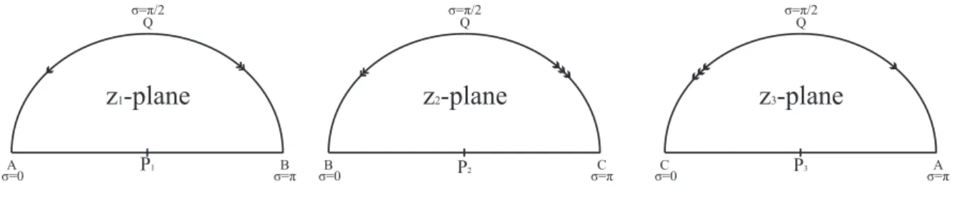
As it is explicit in appendix A, in the z−coordinate system anith string evolving fromt=−∞,
which corresponds to zi = 0 (Pi), propagates radially until it reaches an interaction point, which
6
we considered as t = 0, that is, |zi| = 1. Note that in the CFT framework, these states have
a corresponding vertex operator inserted at Pi. Since we are worried about the 3−string vertex,
the idea is to map the three upper half-disks associated with the strings to one unique disk on a conformal plane. Graphically, we have:
P1
A B
Q
z
1-plane
ó=0 s =ð
s =ð/2
P2
B C
Q
z
2-plane
ó=0 s =ð
s =ð/2
P3
C A
Q
z
3-plane
ó=0 s =ð
s =ð/2
Figure 2.3.: As we learned in the last section, the gluing process will take half of each string and sew together to form a new string-like object.
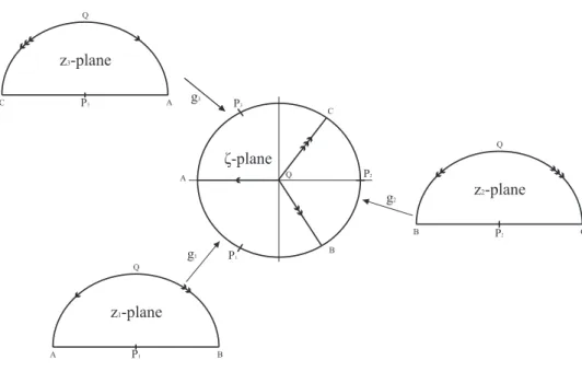
In other words, we will be mapping three half-disks with their own local coordinates zi′s to the interior of a unique disk with global coordinateζ.This map must satisfy these properties:
1. The common interaction pointQis mapped to the center ζ = 0 of the unit disk;
2. The real axes, which are the open string boundaries, are mapped to the boundary of the unit disk.
In order to implement this transformation, let’s consider the first string. The mapping z1 →ω=h(z1) =
1 +iz1
1−iz1
(2.25) satisfy the above properties. On the other hand, we are trying to construct a unit disk from three half disks, so we need to consider yet another transformation over ω so that the the z1−plane is
mapped to a region with an angle of120o. The second transformation is given by
ω→ζ =η(ω) =ω2/3. (2.26)
Following the same ideas for the second and third strings, we end up with three wedges of 120o
angle that can be combined and form a unit disk. The last point to be made is to take care of the sewing, that is, we need to sew together the right-hand piece of the first string with the left-hand piece of the second string and so on, as it was establish in the last section. This can be achieved through the following transformations
g1(z1) = e−
2πi
3
!1 +iz
1
1−iz1
"2/3
η◦h(z2) =g2(z2) =
!1 +iz
2
1−iz2
"2/3
(2.27)
g3(z3) = e
2πi
3
!1 +iz
3
1−iz3
"2/3
P1
A B
Q
z1-plane
P2
B C
Q
z2-plane
P3
C A
Q
z3-plane
?-plane
C
B
A Q
g3
g2
g1
P3
P1
P2
Figure 2.4.:3−string vertex.
Therefore, using those mappings we can give a representation for the interaction term as a
3−point correlator function, ˆ
Φ⋆Φ⋆Φ=+g1◦Φ(0)g2◦Φ(0)g3◦Φ(0)%, (2.28)
where it is defined on the global disk constructed above and evaluated in the combined matter and ghost CFT. Note thatgi◦Φ(0) is just the conformal transformation ofΦ(0)by gi,i.e.
gi◦Φ(0) = (gi′(0))hΦ(gi(0)), (2.29)
if theΦ is a primary operator (A.31) with conformal weighth.
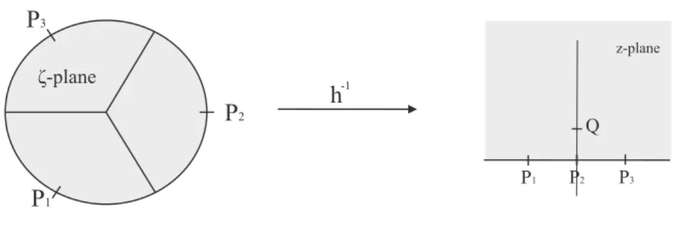
We can now go back to the upper half plane considering the inverse transformation of (2.25), that is,
z=h−1(ζ) =−iζ−1
ζ+ 1, (2.30)
so that the final expression for the3−point vertex is given by
ˆ
Φ⋆Φ⋆Φ = +
3
'
i=1
fi◦Φ(0)% (2.31)
fi(zi) = h−1◦gi(zi). (2.32)
P
3P
2P
1æ-plane
P3
P1 P2
z-plane
Q
Figure 2.5.: Coming back to the upper half plane.
The above construction can be generalized for the n−point vertex, which becomes ˆ
Φ⋆...⋆Φ=+f1◦Φ(0)...fn◦Φ(0)%, (2.33)
where
fj(zj) = h−1◦g(zj)
gj(zj) = e
2πi n (j−1)
(
1 +izj
1−izj
)n2
,1≤j≤n. (2.34)
Hence, for the quadratic term in (2.24) n= 2,so that
f1(z1) = h−1
!1 +iz
1
1−iz1
"
=z1=id(z1) (2.35)
f2(z2) = h−1
!
−1 +1 iz2 −iz2
"
=−1
z2 ≡ I
(z2) (2.36)
and ˆ
Φ⋆QBΦ=+I◦Φ(0)QBΦ(0)%. (2.37)
Finally, the string field theory action in terms of the CFT correlators is given by
S=− 1
g20 *
1
2α′+I◦Φ(0)QBΦ(0)%+
1 3+
3
'
i=1
fi◦Φ(0)%
+
In the last chapter we have constructed an action for the string field considering the axiomatic proposal from Witten’s generalization of the Chern-Simons theory. Besides, we have presented a CFT method to evaluate that action so that one is able to calculate, at least in principle, the full action for the spacetime fields.
Giving our interest in inflation, as we have already stated in the introduction, we will obtain an action for the tachyonic field in a perturbative way, which will be explained below. Then, we will consider its potential calculated in this framework in the last chapter as a candidate for producing an inflationary scenario.
Our basic references are again [3,4,5,6].
3.1. The gauge choice
The action for the bosonic open string theory (2.24) is gauge invariant under the transformation (2.23). Therefore, in order to proceed with our calculations, we will be considering the so called Feynman-Siegel gauge in the state formalism1,
b0|Φ%= 0, (3.1)
that is, there is no c0 mode in the string field. This is a good gauge choice because:
1. It can always be chosen, at least at the linearized level: let’s consider a state |Ψ% with
Ltoto |Ψ% = h|Ψ% not obeying (3.1). We can define a new state |Ψ˜%, which is a linearized
gauge transformation of the original state, as
|Ψ˜%=|Ψ% −1
hQB|Λ%
where|Λ%=b0|Ψ%. The new state satisfies the above gauge condition:
b0|Ψ˜% = b0|Ψ% −
1
hb0QBb0|Ψ%
= b0|Ψ% −
1
hb0{QB, b0}|Ψ%
= b0|Ψ% −
1
hb0L
tot
0 |Ψ%
= 0,
where we have used (B.26) in the third line. Note we have shown this property forh/= 0 and
that the|Ψ˜%and |Ψ%are physically equivalent because, as we have explained in the appendix
B,QB|Λ% is a closed state;
1
2. There are no residual gauge transformations preserving the gauge condition: suppose we have two states satisfying the gauge condition, b0|Ψi%, i = 1,2, and they are related by a gauge
transformation: |Ψ1%=|Ψ2%+QB|ξ%. Therefore,QB|ξ%is a residual gauge degree of freedom.
Then,
h(QB|ξ%) =L0tot(QB|ξ%) ={QB, b0}QB|ξ%=QBb0(QB|ξ%) = 0,
where we have used the nilpotency of QB. Hence, since h /= 0 from above, we see that
QB|ξ%= 0.
Besides, the usefulness of the Feynman-Siegel gauge can be appreciated in the quadratic piece of the action providing the canonical kinetic term for the states satisfying (3.1):
+Ψ1|QB|Ψ2% = +Ψ1|QB{b0, c0}|Ψ2%
= +Ψ1|QBb0c0|Ψ2%
= +Ψ1|{QB, b0}c0|Ψ2%
= +Ψ1|Ltot0 c0|Ψ2%
= +Ψ1|c0Ltot0 |Ψ2%,
where we used again (B.26) and [Ltot
0 , c0] = 0. As L0tot is roughly p2+m2, we have the familiar
kinetic terms.
3.2. Level truncation scheme
As we have defined in the last chapter, the string field has infinite spacetime fields in it. Hence, in order to work out the action (2.24) we have to developed some kind of truncation.
Let’s expand|Φ% in the momentum basis using the state formalism, so
|Φ% =
ˆ ddk
!
ϕ+Aµαµ−1+iαb−1c0+√i
2Bµα
µ
−2+
1
√
2Bµνα
µ
−1αν−1
+β0b−2c0+β1b−1c−1+iκµαµ−1b−1c0+...,c1|k%, (3.2)
where we have not considered a gauge condition yet. The expansion coefficients might appear to
be quite arbitrary, but they are adjusted so that the spacetime field terms recover their usual form in the end. Now, remembering from appendixA, we know that
Ltot0 =α′p2+
∞
-n=1
αµ−nαµn+
∞
-n=−∞
n◦c−nbn◦ −1, (3.3)
where ◦...◦ denotes annihilation-creation normal ordering. Then, we define thelevel of a state as the sum of the level numbers n of the creation operators acting on c1|k%,that is, the sum of the
second and third terms above. Therefore, the zero momentum tachyonic mode has level 0.
We can also define the level of each term in the action, which is naturally defined to be as the sum of the level of each field involved. Therefore, we understand the truncation to level N as keeping only those terms with level less than or equal to N. We shall denote “level (M, N) truncation” when the string field has terms with l≤M while the action has ones with l≤N.
Another important point to be made is that when a particular level truncation is chosen the gauge invariance breaks down because the action was invariant under the full gauge transformations, which involves all the infinite fields. Hence, in order to proceed with calculations, we shall impose our gauge choice before use the level truncation.
3.3. The potential
In this section we intend to obtain a formula for the tachyonic potential using the methods developed above and results from appendix A so that we can consider it as a candidate for producing an inflationary scenario. Since our objective here is academic, we will keep the calculations as simple as we can using the very first approximation that the level truncation scheme provides us. As we have talked above, the string field has an infinite number of spacetime fields which can be classified according to their level. In order to do calculations, we use the level truncation scheme as an approximation. For our purposes here, let’s consider the |Φ% up to l= 2. Besides, we work in the
Feynman-Siegel gauge, thus all the terms containingc0 are dropped. Therefore, (3.2) becomes
|Φ%=
ˆ ddk
.
ϕ(k) +Aµ(k)αµ−1+
i
√
2Bµ(k)α
µ
−2+
1
√
2Bµν(k)α
µ
−1αν−1+β1(k)b−1c−1
/
c1|k%. (3.4)
Using the vertex-operator map from section A.5, we can rewrite the string field in the operator formalism as
|Φ% =
ˆ ddk
.
ϕ(k)c(0) +√i
2α′Aµ(k)c∂X
µ(0)
− 1
2√α′Bµ(k)c∂
2Xµ(0)
− 1
2√2α′Bµν(k)c∂X
µ∂Xν(0)
−12β1(k)∂2c(0)
/
|k%, (3.5)
with |k% = eik·X(0)|0%. As one can check, the vertex operators of the last three terms above are
not primary operators (A.31) and they can complicate a lot the CFT method. Therefore, we will proceed with our calculations at the(1,3)truncation level.
The quadratic term in (2.24) is +I ◦Φ(0)QBΦ(0)%, then we have to consider the conformal
transformations of the vertex operators in the string field underI=−z−1 given by (A.31), so that 1. I ◦0ceik·X(ǫ)1=
=
.
∂z
!
−1z
"/−1+α′k2
z→ǫ
ceik·X !
−1ǫ
"
=
!1
ǫ2
"−1+α′k2 ceik·X
!
−1ǫ
"
; (3.6)
2. I ◦0c∂Xµeik·X(ǫ)1=
=
.
∂z
!
−1z
"/−1+α′k2+1
z→ǫ
c∂Xµeik·X !
−1ǫ
"
=
!1
ǫ2
"α′k2
c∂Xµeik·X !
−1ǫ
"
Note that we have to take the limit ǫ → 0 in the end. Then, using (B.24), the quadratic term
becomes
+I ◦Φ(0)QBΦ(0)% =
ˆ
ddkddq 2*!1
ǫ2
"−1+α′k2
ceik·X !
−1ǫ
" ϕ(k)+
i
√
2α′Aµ(k) !1
ǫ2
"α′k2
c∂Xµeik·X !
−1ǫ
"+˛ dz
2πi[cT
m(z) +bc∂c(z)]
×
.
ϕ(q)ceiq·X(ǫ) +√i
2α′Aν(q)c∂X
νeiq·X(ǫ)/3 ǫ→0
=
ˆ
ddkddq ˛
dz
2πi 2!
1
ǫ2
"−1+α′k2 ϕ(k)
.
ϕ(q)ceik·X !
−1ǫ
"
cTm(z)ceiq·X(ǫ)
+√i
2α′Aν(q)ce
ik·X!−1
ǫ "
cTm(z)c∂Xνeiq·X(ǫ) +ϕ(q)ceik·X !
−1
ǫ "
bc∂c(z)ceiq·X(ǫ)
+√i
2α′Aν(q)ce
ik·X!−1
ǫ "
bc∂c(z)c∂Xνeiq·X(ǫ)
/
+√i
2α′Aµ(k) !1
ǫ2
"α′k2
×
.
c∂Xµeik·X !
−1ǫ
"
cTm(z)ceiq·X(ǫ)ϕ(q) +√i
2α′Aν(q)c∂X
µeik·X!−1
ǫ "
cTmc∂Xνeiq·X(ǫ)
+ϕ(q)c∂Xµeik·X !
−1ǫ
"
bc∂c(z)ceiq·X(ǫ) +√i
2α′Aν(q)c∂X
µeik·X!−1
ǫ "
bc∂c(z)c∂Xνeiq·X(ǫ)
/3
ǫ→0 .
We have eight different terms above, but we will keep our attention to the ones involving only the
tachyonic field2
. Therefore, we are left with
+I ◦Φ(0)QBΦ(0)%ϕ =
ˆ
ddkddq
˛ dz
2πi
!1
ǫ2
"−1+α′k2
ϕ(k)ϕ(q)
45
ceik·X
!
−1ǫ
"
cTm(z)ceiq·X(ǫ)
3
+
5
ceik·X
!
−1
ǫ "
bc∂c(z)ceiq·X(ǫ)
36
. (3.8)
The detailed calculation is presented in appendixC. The final result is
+I ◦Φ(0)QBΦ(0)%ϕ = (2π)dα′
ˆ
ddk
!
k2− 1
α′ "
ϕ(−k)ϕ(k). (3.9)
Considering the Fourier-transformation to the position space,
ϕ(k) =
ˆ ddk
(2π)dϕ(x)e
−ik·x, (3.10)
the quadratic part of the tachyonic field becomes
Sϕ(2)= 1
g02
ˆ
ddx
!
−1
2∂µϕ∂
µϕ+ 1
2α′ϕ
2". (3.11)
2
Now, let’s calculate the cubic term. We will focus again on the terms of our interest, that is, involving only the scalar field. Even though just the main results are expressed below, we provide details in appendix C. From (2.31), we consider
fi◦Φ(0) =
ˆ ddk
.
ϕ(k)fi◦(ceik·X)(0) +
i
√
2α′Aµ(k)fi◦(c∂X
µeik·X)(0)/
=
ˆ
ddk78fi′(0)9α′k2−1ϕ(k)ceik·X(fi(0))
+ √i
2α′ 8
fi′(0)9α′k2Aµ(k)c∂Xµeik·X(f′(0))
6 . Then, we need to calculate the f′
isand their first derivatives. They are given by
w1 = − √
3
w2 = 0
w3 = √
3
w1′ = 8 3
w2′ = 2 3
w3′ = 8 3,
wherewi ≡fi(0).The3−point function has only one term involving only the tachyonic field, which
is
+ 3
'
i=1
fi◦Φ(0)% =
ˆ ddk
ˆ dpk
ˆ
ddqw1′α′k2−1w2′α′p2−1w3′α′q2−1ϕ(k)ϕ(p)ϕ(q)×
:
ceik·X(w1)ceip·X(w2)ceiq·X(w3)
;
= (2π)d
ˆ ddk
ˆ ddp
ˆ
ddqw1′α′k2−1w2′α′p2−1w3′α′q2−1ϕ(k)ϕ(p)ϕ(q)×
|w12|2α
′k·p+1
|w23|2α
′p·q+1
|w13|2α
′k·q+1
= 6√33
3
27(2π)
dˆ ddkˆ dpkˆ ddqδd(k+p+q)ϕ(k)ϕ(p)ϕ(q)F(k, p, q),(3.12)
where
F(k, p, q) = exp
. α′ln
! 4
3√3
"
(k2+p2+q2)
/ . Thus, theϕ3 term in the action is given by
Sϕ(3) =− 1 3g2
0
(
3√3
4
)3ˆ
ddxϕ˜(x)3, (3.13) where we have used the Fourier-transformation for the position space (3.10) and defined
˜
ϕ(x) = exp
!
−α′ln 4
3√3∂µ∂
µ"ϕ(x). (3.14)
Therefore, the tachyonic action3 is given by Sϕ=
1
g02 ˆ
ddx
−1
2∂µϕ∂
µϕ+ 1
2α′ϕ
2−1
3
(
3√3
4
)3
˜
ϕ3
. (3.15)
3
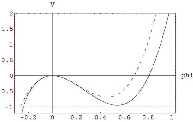
There are higher-order calculations in the literature, up to level (10,20) [36]. In order to see
how good is the approximations we have considered above, let’s write the effective potential for the (2,4)−level [4]:
V(2,4) = 6π
2ϕ2
256(288 + 581√3ϕ)2(432 + 786√3ϕ+ 97ϕ2)2 ×
×(−660451885056−4510794645504√3ϕ
−32068942626816ϕ2−25455338339328√3ϕ3+ 27487773823968ϕ4
+54206857131636√3ϕ5+ 24845285906980ϕ6+ 764722504035√3ϕ7). (3.16)
The graphic of the potential in the level we calculated, which was(0,0)after all the approximations,
and the level(2,4)is [4]
Figure 3.1.: The dashed line is the potential calculated here while the solid line is the potential for the(2,4)level.
and old approaches
Before we start to study inflation and its consequences, it is important to contextualize the sta-tus quo of cosmology by the end of 70′s, focusing in its properties and issues that preceded and motivated the inflationary scenario proposal. Some points of the discussion will be limited to qual-itative aspects, hence the reader that is not familiar with General Relativity or the basic aspects of Cosmology should first address the appendixD.
4.1. Historical Context
The cosmological standard model before the inflationary proposal by [15, 16, 17, 23] had some arguable problems related with initial-conditions. After the observation of the CMB (Comic Mi-crowave Background) radiation, which indicated that the universe was extremely homogeneous and isotropic at recombination1, the best model at time to describe the primordial universe until the CMB emission was provided by the expanding radiation-dominated FRW metric2.
On the other hand, we know that inhomogeneities are unstable gravitationally (if there is an accumulation of matter-energy at some point, this should grow with time because gravity is at-tractive). As a result, if the CMB pointed out a universe highly homogenous at the last-scattering surface, it was expected that the inhomogeneities were even smaller in the primordial universe. However, Rindler [18] had already noticed that an expanding radiation-dominated universe should have a particle horizon and, consequently, it would be composed of a lot of causally disconnected regions. Therefore, it is odd to imagine that these regions should present so similar physical proper-ties without any dynamical reason. This is essentially the recipe for the initial-condition problems we will talk quantitatively below.
4.2. A simple analogy
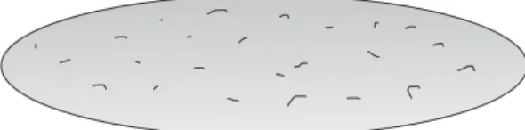
It is generally better when we can have some intuition about a complicated problem using ordinary physics. Hence, let’s consider the following situation: suppose we receive a photograph of a very soft material, showing the shape in the Figure4.1.
1
Footnote on page67.
2
Figure 4.1.: Note that the shape presented is very flat and regular, with only some small "inhomo-geneities" in its surface.
Knowing that it could be anything in the photo (it is a soft object after all), we could ask ourselves some natural questions: why such a regular object? Why is it so flat? Then, one may consider two different positions: the object was always just as above and that is it, or something
might have happened to make the object as in the figure. In this very simple case, one who has chosen the second alternative might wonder that a racket have hit the object, Figure4.2, letting it as above.
(a) (b) (c)
Figure 4.2.: (a) Very irregular object; (b) Ping-Pong racket hitting the material; (c) The material is deformed in a very regular form.
Well, what any of this has anything to do with the universe? Actually, it is pretty much the same physical intuition. Take the very irregular soft material as some initial state of the universe at a very early age, which was inhomogeneous. The photograph is representing the CMB, which tells us the universe was extremely homogeneous and isotropic, i.e., the analogous to the object soon after being hit. Besides, the questions posed above can be translated as: why the universe was very homogeneous and isotropic? Why was it so flat? And the answer for both situations could be a very short period of acceleration, that is, a racket hit causing a stretching acceleration on the object and a very short period of accelerated expansion of the universe, also known as inflation.
Therefore, inflation will be understood as a stage of accelerated expansion of the universe in the very early ages. It will be argued quantitatively and qualitatively that it can address some initial-condition problems once one has assumed that Quantum Gravity is not relevant3 after
tP l∼10−43s
and that inhomogeneities are not dissolved by expansion.
Before we continue, one should note that the problem to explain dynamically the initial-conditions of the universe, its kinematics, is essentially a philosophical one. When some of the others areas are
3
contemplated, coming from classical mechanics to quantum physics, we see that the dynamics is fundamentally concerned in predicting the future evolution of a system given the initial-conditions. Hence, it is not clear if cosmology should differ from this paradigm. On the other hand, once we
have a dynamical theory in which these conditions are naturally produced, we shall explore it and try to infer some other results in order to corroborate this scenario.
4.3. The initial-condition issues
In this section, we will follow some calculations from [10] with minor changes and present some insights coming from different references which are cited in the text.
4.3.1. Homogeneity, isotropy (horizon) problem
The homogeneous and isotropic wedge of the universe at the last-scattering surface is at least as large as the horizon scale: ctrec∼1021m(it is bigger if taking into account that it was expanding),
wheretrec is 380,000years.
Initially, this piece of the universe was much smaller, by a factor4 of ai
arec.Hence, the size of the
isotropic homogeneous region from which the universe at the last-scattering originated at t = ti
was of order
li ∼ctrec
ai
arec
. (4.1)
On the other hand, the causal region at that time was of orderlc ∼cti (in fact, it would be smaller
if we considered the expansion). Comparing both regions, li
lc ∼
trec
ti
ai
arec
. (4.2)
In order to estimate this ratio, we assume that the primordial radiation dominates atti ∼102×tP l
and use that a(t)∝t12 from Table D.1. Hence, li
lc ∼
10−1
@ trec
tP l
∼10−1 @
1013
10−43 ∼10
27. (4.3)
Thus, at ti the size of the homogeneous and isotropic universe exceeded the causality scale by
27 orders of magnitude! This means that in 1081 (volume ∼ l3) causally disconnected regions the energy density was distributed with a fractional variation not exceeding δρ/ρ ∼ 10−4. This unnatural fine-tunning energy distribution cannot be explained by causal physical processes given that no signals propagate faster than light.
Note also that if a∼tn,then a
t ∼a˙ and (4.2) becomes
li
lc ∼
˙
ai
˙
arec
, (4.4)
which implies that the homogeneity scale was always larger than the causality one if gravity was always attractive (hence decelerating the expansion). That’s why this problem is also calledhorizon problem.
An important point to be made that was emphasized by Guth [15] is that the horizon problem could be obviated by consideration of the full quantum gravitational theory if it has an unexpected behavior in the very early universe, which could compensate this huge scale difference between the causal connected regions and their homogeneity.
4
4.3.2. Flatness problem
One of the Friedmann equations from General Relativity is given by (D.32)
H2+ k
a2 =
8πρ
3 , (4.5)
where H(t) = aa˙((tt)) is the Hubble parameter, k is associated with the spatial curvature and ρ(t) is the energy density. We define the cosmological parameter,Ω(t), as
Ω(t) = ρ(t)
ρcr(t), (4.6)
where ρcr(t) = 3H2/8π is the critical energy (it is often used to refer to the current value of the energy density). Then (4.5) can be rewritten as
Ω(t)−1 = k
(Ha)2. Thus,
Ωi−1 = (Ωrec−1)
(Ha)2rec (Ha)2
i
= (Ωrec−1)
!a˙
rec
˙
ai
"2
≤10−54, (4.7)
where we have used (4.4) and Ωrec ≅15. Hence, the above relation tells us that the cosmological
parameter must be initially extremely close to unity, i.e., we had a flat universe by that time. That’s why we call this as the flatness problem. It was known at least since the end of70′s [19].
4.3.3. Initial perturbation problem
One might wonder how the primordial inhomogeneities that ended up forming the large structures of the universe were originated. An answer to this question is also expected and it turns out that inflation has something to say about it. In fact, inflation might not only be responsible for the large-scale homogeneity of the universe, but also for the small fluctuations in the primordial universe that were the seeds for the formation of the large-scale structures.
A qualitative understanding [12] is to imagine that the microscopic fluctuations in the energy density were created in the very early universe during a period of inflation. Then, they were stretched by the inflationary expansion to macroscopic scales, larger than the physical horizon at that time, leaving behind a perfectly homogeneous universe. These perturbations remained causally unaccessible until they re-enter the horizon at a later time during the FRW non-accelerated expansion, when the universe was about100,000years old, before recombination. Inside the horizon again, these perturbations could create the inhomogeneities we observe in the CMB spectrum that were the key for the large-structure formation.
This is all we will talk about cosmological perturbations. The interested reader can check [12,10] for more informations.
4.4. Inflation: qualitative aspects
In the last section we saw that the initial-condition problems are related to the fact thata˙i/a˙rec ≫1.
This condition can be avoided only if during some period of expansion gravity acted as a repulsive
5
In order to check this, we can use (4.7) withti→t0 =today andΩ0 =−0.001 !
+0,0062
−0,0065 "
from [14]. The
force, thus accelerating the expansion. In this situation, we can have a˙i/a˙rec <1 and it becomes
possible to have a large homogeneous universe coming from a single causally connected domain. This is a necessary but not suficient condition. Despite of general features of inflation that can be investigated, the specific model that provides this scenario will also play an important role, as we will be able to see studying the old, new and chaotic inflationary scenarios in the next sections and chapter.
Considering the above remarks, inflation is a stage of accelerated expansion of the universe when gravity acts as a repulsive force. The general picture of universe evolution in its early ages should be as the Figure4.3,
QG?
a
t tf
inflation
decelerated Friedmann expansion
Figure 4.3.: Representation of what the expansion of the universe would look like in the first ages, where tf ∼10−34−10−36s. QG stands for Quantum Gravity.
where tf comes essentially from requiring the generation of primordial fluctuations. We also note
that the curve is smooth at the connection between the end of inflation and the Friedmann expan-sion. This is important to guarantee that the homogeneity of the universe is not spoiled.
The idea of an accelerated expansion phase in the beginning of the universe is, in fact, better than stated above because it is even possible to relax the restriction of homogeneity on the initial conditions, i.e., if starting with a strongly inhomogeneous causal domain, inflation can produce a large homogeneous universe (intuitively, it is possible to think of a very irregular rubber material being suddenly stretched). A quantitative argument is given at [10], page 232. This is one of the aspects regarding chaotic inflation, as we will see in chapter5.
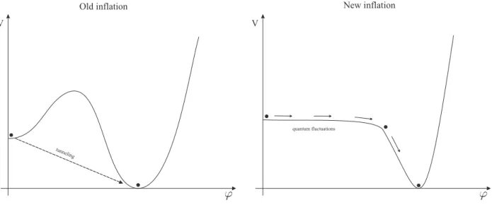
4.5. The old and new scenarios
Let’s now consider the initial proposals of an inflationary universe, first Guth’s and Sato’s [15,23], known as the old inflation, and then Linde’s [16] and Steinhardt and Albrecht’s [17], called new inflation.
4.5.1. The old inflation

![Figure 5.4.: From [22 ], we have f ≈ 10 19 GeV and m ≈ 10 16 GeV , so that in Planck units we consider f = 50 60 and m = 12201](https://thumb-eu.123doks.com/thumbv2/123dok_br/15760184.128217/45.892.257.658.542.855/figure-f-gev-m-gev-planck-units-consider.webp)
