Structural analysis of the timber structure of Ica Cathedral, Peru

(1)

| 2015

UNIVERSITAT POLITÈCNICA DE CATALUNYA

Maria Pia Ciocci

Structural Analysis of the Timber

Structure of Ica Cathedral, Peru

Maria Pia Ciocci

Str uctur al Anal ysis of t he T imber Str uctur e of Ica Cat hedr

(2)

Structural Analysis of the Timber

Structure of Ica Cathedral, Peru

(3)

Name: Maria Pia Ciocci

Email: mariapiaciocci@gmail.com

Title of the Msc Dissertation:

Structural Analysis of the Timber Structure of Ica Cathedral, Peru

Supervisor(s): Paulo B. Lourenço, Elisa Poletti

Year: 2015

I hereby declare that all information in this document has been obtained and presented in accordance with academic rules and ethical conduct. I also declare that, as required by these rules and conduct, I have fully cited and referenced all material and results that are not original to this work.

I hereby declare that the MSc Consortium responsible for the Advanced Masters in Structural Analysis of Monuments and Historical Constructions is allowed to store and make available electronically the present MSc Dissertation.

University: University of Minho

Date: 07 / 09 / 2015

Signature:

(4)

(5)

Acknowledgements

I would like to express my great appreciation to my supervisors.

My sincere gratitude to Prof. Paulo Lourenço for this exceptional challenge. His inspiring guidance and enthusiasm to discuss every single idea were essential in each step of this work.

I would like to acknowledge Elisa for her continuous help and patience.

I would like to profusely thank the European Commission for the financial support without which this fulfilling experience would not have been possible.

I am very grateful to everyone who ran this great SAHC marathon with me.

A special thanks to who discussed FEM while I was brushing my teeth, to who helped me day by day and to who made me feel at home.

Thanks to the special friend who has shared this entire journey with me, for all the discussions and for all the smiles shared.

A special thanks to who has encouraged me since the first day of this experience.

As usual, my deepest gratitude to my family and my friends who always supports me without any hesitation.

(6)

(7)

Abstract

The Cathedral of Ica, built in 1759 and damaged by the 2007 Pisco earthquake, is one of the most representative of the churches built in coastal cities of Peru. Declared as national monument in 1982, Ica Cathedral is part of the Seismic Retrofitting Project of the Getty Conservation Institute.

Two structural systems are present in Ica Cathedral. At the exterior, a massive and stable load– bearing masonry envelope surrounds the cathedral consisting of the fired brick front façade with two bell towers and thick mud brick lateral walls. On the other hand, the internal space of Ica Cathedral is divided by a series of pillars that support a complex vaulted roof framing system constructed with the quincha technique. In particular, the latter is the main object of this thesis.

The important influence of timber connections on the global behaviour of timber structures is investigated by modelling a timber frame wall, analytically and numerically. The architecture, the structural systems and recent damage of Ica Cathedral are presented in details with the construction of 3D–architectural models in AutoCAD. Performing linear elastic analyses on the model of the representative bay in SAP 2000 software, the compliance with the criteria specified by Eurocode is evaluated. Finally, the elastic behaviour of the complete timber structure is investigated by constructing a model in MIDAS FX+ for DIANA software.

The results obtained from this thesis represent a starting point for the further research on the numerical model of the combined timber and masonry structures of Ica Cathedral.

(8)

(9)

Resumo

A Catedral de Ica, construída em 1759 e danificada pelo terremoto de Pisco em 2007, é uma das mais representativas igrejas construídas nas cidades costeiras do Peru. Declarada como monumento nacional em 1982, a Catedral de Ica é parte do projeto Seismic Retrofitting Project do Getty Conservation Institute.

Dois sistemas estruturais estão presentes na Catedral de Ica. No exterior, uma massiva e estável alvenaria estrutural envolve a catedral, consistindo numa fachada frontal em tijolo com duas torres e as paredes laterais de elevada espessura compostas por alvenaria de adobe. Por outro lado, o espaço interno da catedral é dividido por uma série de pilares que suportam a estrutura da cobertura que é composta por um complexo sistema abobadado construído com a técnica de quincha. Em particular, este último é o principal objeto desta tese.

A importante influência das ligações de madeira no comportamento global das estruturas de madeira é investigada através da modelação de uma parede de estrutura de madeira, analiticamente e numericamente. A arquitetura, os sistemas estruturais e os danos recentes observados na catedral são apresentados em detalhe com modelos arquitetónicos 3D executados em AutoCAD. Foram realizadas análises elásticas lineares de um modelo representativo da estrutura através do software SAP 2000, avaliando a conformidade com os critérios especificados pelo Eurocode. Finalmente, o comportamento elástico de toda a estrutura de madeira é investigado através da construção de um modelo em MIDAS +FX para o software Diana.

Os resultados obtidos com esta tese representam um ponto de partida de um modelo combinado de madeira e alvenaria para a Catedral de Ica.

(10)

(11)

List of Figures

Figure 1. Geometry of the timber frame wall specimen. ... 5

Figure 2. Timber frame wall with lower (left) and higher (right) vertical load levels (Poletti, 2013). .... 8

Figure 3. Typical damage of the connections. ... 9

Figure 4. Axial and shear stiffness for the connection between the diagonals and the main frame. .. 13

Figure 5. Contact areas of the connections by contact. ... 14

Figure 6. Rotational stiffness for the half–lap connection. ... 16

Figure 7. Schematic of the numerical model. ... 17

Figure 8. Typical cell for each numerical model. ... 18

Figure 9. Linear elastic force–deformation for Link 1 in MOD 2. ... 19

Figure 10. Linear and nonlinear elastic force–deformation for Link 1 and Link 2 in MOD 3. ... 20

Figure 11. Deformed shape (left) and axial force diagram (right) of MOD 0. ... 22

Figure 12. Force–displacement for the half–lap connection. ... 24

Figure 13. Moment–rotation for the half–lap connection. ... 24

Figure 14. Parametric analysis on the capacity of the connection between the diagonals and the main frame. ... 26

Figure 15. Parametric analysis on the stiffness of the connection between the diagonals and the main frame. ... 26

Figure 16. Influence of shear stiffness in nonlinear analysis. ... 27

Figure 17. Influence of the shear stiffness. ... 28

Figure 18. Summary of the capacity curves obtained from the modelling of the timber frame wall. . 31

Figure 19. The front façade (left) (Cancino, et al., 2012) and the current condition of the internal space of Ica Cathedral (Image: https://www.flickr.com/people/thegetty/). ... 34

Figure 20. Satellite image (left) (2015 Google. Image 2015 Digital Globe) and the location of Ica Cathedral (right) (Garcia Bryce & Soto Medina, 2014). ... 35

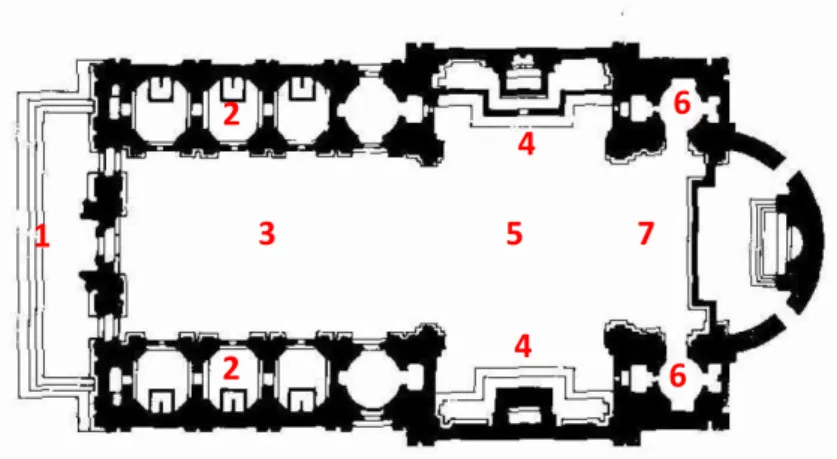
Figure 21. Schematic plan of the Church of Gesù in Rome: atrium (1), side aisles (2), main nave (3), arms of the transept (4), crossing of the transept (5), chapels (6) and altar (7). ... 36

Figure 22. Schematic of the plan of Ica Cathedral: atrium (1), main entrance (2), main nave (3), side aisles (4), crossing of the transept (5), arms of the transept altar (6), altar (7) and chapels (8). ... 37

(14)

vault (orange), main dome (dark blue), aisles’ domes (light blue), cross ribs vaults (green) and flat ceiling (white). ... 38

Figure 24. Pillars of Ica Cathedral: pillar of the crossing (green), nave pillar (red), pilaster (blue) and

pier (orange) (Cancino, et al., 2012). ... 40

Figure 25. (A) Pillar of the crossing (Image: Emilio Roldán Zamarrón for GCI), (B) Nave pillar, (C)

Pilaster with the pier behind. ... 40

Figure 26. Couples of wooden frameworks between nave pillars (red), nave pillar and pilaster (blue)

and pillar of the transept and pilaster (green). ... 41

Figure 27. Schematic of the horizontal elements of Ica Cathedral: longitudinal beam (blue),

transversal beam (red) and connection between timber and masonry structures (orange). ... 41

Figure 28. Schematic of the vaulted roof framing system of Ica Cathedral: principal arch (red),

secondary arch (orange), vertical and horizontal ribs of the main dome (blue), ribs of the aisle’s dome (green) and flat ceiling (purple). ... 42

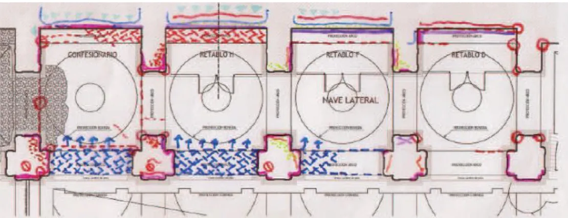
Figure 29. Graphic condition survey of the south side aisle: humidity (light blue arrows), vertical

cracks (red circles), horizontal crack (red line), partial collapse (red hatch pattern), out-of plane displacement (dark blue hatch pattern and dark blue arrows) (Cancino, et al., 2012). ... 43

Figure 30. Graphic condition survey of the main nave: termite damage (green line), partial collapse

(red hatch pattern), cracking (red line) (Cancino, et al., 2012). ... 44

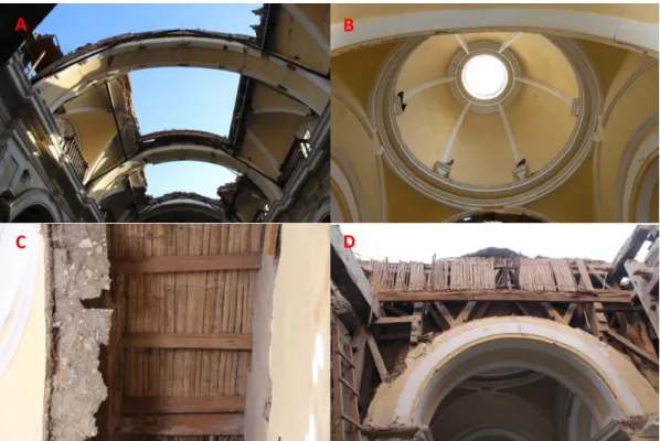
Figure 31. (A) Partial collapse of the barrel vaults (Image: Emilio Roldán Zamarrón for GCI), (B)

Mortise and tenon connections at the top of the lunette (Image: Emilio Roldán Zamarrón for GCI) (C) Corrosion of the nailed connection of the arches of the barrel vaults (Cancino, et al., 2012) (D) Detail of the lunette’s beam (Cancino, et al., 2012). ... 45

Figure 32. (A) and (B) Partial collapse of the main dome after the 2007 Pisco earthquake (Cancino, et

al., 2012), (C) and (D) Total collapse of the main dome actually. ... 45

Figure 33. The main parts of the representative bay: (A) Barrel vault with lunettes, (B) Aisles’ domes,

(C) Aisles’ joists and (D) Timber framework. ... 47

Figure 34. Survey of the nave pillar: (A) View of the nave pillar, (B) Connection between the posts and

the fire brick base and (C) Detail of the huarango trunk tree. ... 48

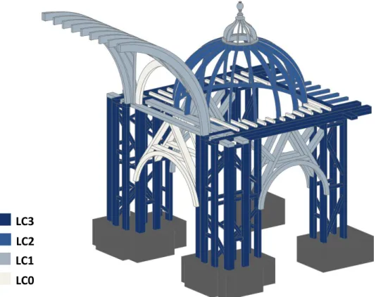
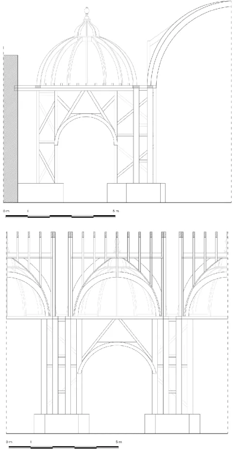
Figure 35. Mapping of the levels of confidence for the representative bay. ... 50 Figure 36. Characterization of the pilaster (top) and the nave pillar (bottom). ... 51 Figure 37. Ground plan (top) and roof plan (bottom) of the representative bay of the Ica Cathedral. 52

(15)

Cathedral. ... 53

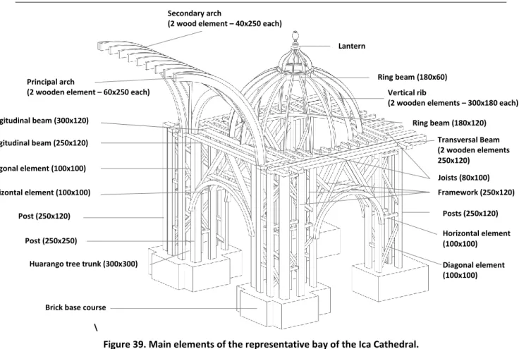
Figure 39. Main elements of the representative bay of the Ica Cathedral. Note that the dimensions are in mm. ... 54

Figure 40. Posts and horizontal elements of the central pillar (Image: Emilio Roldán Zamarrón for GCI). ... 56

Figure 41. Main elements of the representative bay of the Ica Cathedral. Note that the dimensions are in mm. ... 57

Figure 42. 3D architectural AutoCAD mode (left) and the discretized model in AutoCAD (right). ... 60

Figure 43. FE mesh in SAP 2000. ... 61

Figure 44. Assumptions on the covering layers on the timber structure (Garcia Bryce & Soto Medina, 2014). ... 65

Figure 45. Deformed shape of the structure under the load combination for ULS. ... 67

Figure 46. Distribution of axial forces in the structure under the load combination for ULS. ... 68

Figure 47. Sets of timber connections for parametric analyses performed on SB 1, SB 2 and SB 3. ... 69

Figure 48. Capacity curves obtained from parametric analysis on the connections of the representative bay. ... 70

Figure 49. Capacity curves obtained from parametric analysis on the connections of the barrel vault. ... 71

Figure 50. Factors used for the calculation of the effective lengths of column. ... 79

Figure 51. Beam at the top of the lunettes and its mortise and tenon connections... 87

Figure 52. Distribution of the stresses in the beam at the top of the lunettes. ... 89

Figure 53. Configuration of sectors used of the numerical model. ... 94

Figure 54. Numerical model of the complete timber structure of Ica Cathedral. ... 97

Figure 55. Vertical displacements of the timber structure of Ica Cathedral under self-weight. ... 99

Figure 56. Deformation under lateral loading ±YY direction. ... 102

Figure 57. Deformation under lateral loading –XX direction ... 102

Figure 58. Deformation under lateral loading ±YY direction ... 102

(16)

List of Tables

Table 1. Timber material properties (Poletti, 2013). ... 6

Table 2. Significant values for the envelope curves (Poletti, 2013). ... 10

Table 3. Axial and shear stiffness for the connection by contact. ... 14

Table 4. Axial and shear stiffness for the connection by contact. ... 15

Table 5. Rotational stiffness for the half–lap connection. ... 16

Table 6. Results of the numerical model MOD 2. ... 23

Table 7. Results of the linear elastic analysis on MOD 3. ... 24

Table 8. Parametric analysis on the connection between the diagonals and the main frame. ... 26

Table 9. Influence of shear stiffness in nonlinear analysis. ... 27

Table 10. Stiffness values obtained from the analytical model. ... 29

Table 11. Comparison between the models with rigid and hinged connection. ... 29

Table 12. Calibration of the axial stiffness in MOD 2 and MOD 3. ... 30

Table 13. Seismic events that have affected Ica Cathedral... 35

Table 14. Connections of the representative bay in Ica Cathedral. Note that the letters in the brackets refer to Figure 33. ... 47

Table 15. Distribution of the wood species throughout the representative bay. ... 48

Table 16. Approximate cross section dimensions of the posts of the nave pillar (Greco, et al., 2015). ... 49

Table 17. Possible connections of the transept in Ica Cathedral. ... 55

Table 18. Possible distribution of the wood species throughout the transept... 55

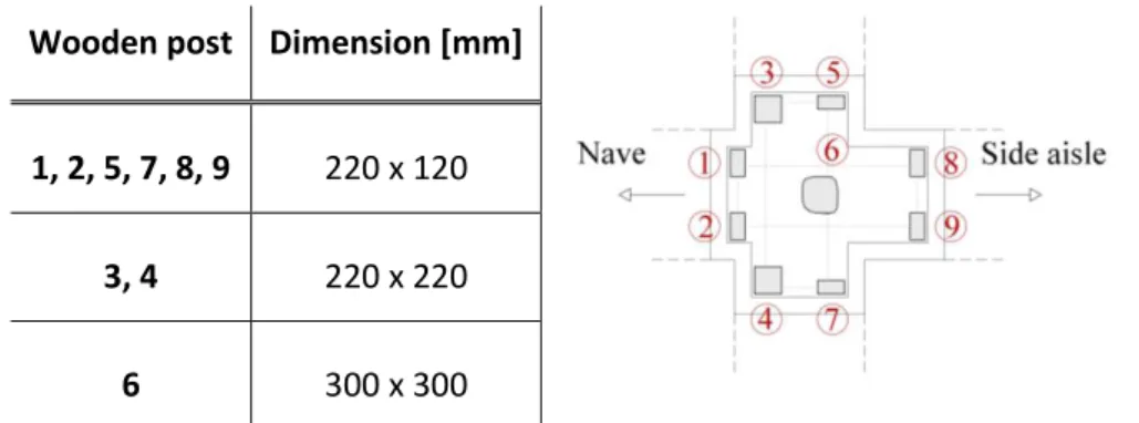
Table 19. Configuration and cross section dimensions of the posts of the central pillar (Greco, et al., 2015). ... 56

Table 20. Characterization of the horizontal connections of the central pillar (Greco, et al., 2015). .. 57

Table 21. Mean values of properties of the wood species by PUCP (GCI & PUCP, 2014). ... 62

Table 22. A summary of the geometrical and material properties for the model of the representative bay. ... 65

(17)

bay. ... 66

Table 25. Absolute maximum values of internal forces and displacements for different loading scenarios. ... 68

Table 26. Values of global structural stiffness obtained using a parametric analysis on timber connections. ... 70

Table 27. Values of stiffness obtained from parametric analysis on timber connections of the barrel vault. ... 71

Table 28. Values of stiffness obtained from parametric analysis on timber connections. ... 72

Table 29. Design values adopted for the different wood species. ... 75

Table 30. Values of for rectangular cross sections (Garbin, 2015). ... 77

Table 31. Verification for ULS of the beam at the top of the lunette according EC 5 (2004). ... 83

Table 32. Verification for ULS of the transversal beam according EC 5 (2004). ... 84

Table 33. Verification of a post of the pilaster with the criteria for ULS according EC 5(2004). ... 85

Table 34. Verification for SLS of deformations according EC5 (2004). ... 86

Table 35. Verification of the connections under the load combination for ULS. ... 88

Table 36. Verification of the beam at the top of the lunettes under the load combination for ULS. .. 89

Table 37. Verification of the connections under the load combination G+1.5E. ... 90

Table 38. Verification of the beam at the top of the lunettes under the load combination G+1.5E. .. 90

Table 39. A summary of the geometrical and material properties for Sector C. ... 96

Table 40. A summary of the geometrical and material properties for the model of sector A and D. .. 96

Table 41. Absolute maximum error considering different elements in DIANA. ... 98

Table 42. Values of stiffness considering different structural parts [g/m]. ... 101

(18)

(19)

Chapter 1

1. Introduction

Efficient restoration and conservation studies of architectural heritage cannot be carried out without a proper evaluation of the structural behaviour. The aim of this thesis is to investigate the complex and unique timber structure of Ica Cathedral in Peru.

In the interior, Ica Cathedral is divided by a series of pillars, pilasters and piers that support a complex roof framing system. These structural parts are essentially hollow structures constructed by applying the quincha technique. The technique of quincha, or bahareque, construction is common in Central America and the South American countries. Although in each country the process varies because of the types of local materials available, the fundamentals of the method are the same (Carbajal, et al., 2005): connected timber elements are covered with cane or small branches forming a single or double–stuffed mesh. The mesh is made of mud, earth, plaster (mixture of lime and water), or a combination of such materials. Timber elements made of different wood species (cedar, sapele and huarango) and connected by various timber connections (mainly, mortise and tenon and half–lap joints) are used to construct the hollow structures that are present in Ica Cathedral. Caña

chancada (wrap with flattened cane reeds) and caña brava (cane reeds) are the particular covering

layers used for these elements (Cancino, et al., 2012). This timber structure of Ica Cathedral represents an extraordinary example of the application of quincha technique. It should be mentioned

(20)

Erasmus Mundus Programme

that while many examples of timber frame walls constructed with quincha technique exist, its application to the curved roof framing system represents an exception that must be preserved. The main objective of this work is to assess the structural performance of the timber structure with a proper investigation of the architecture and the structural systems that are present in Ica Cathedral. The structural behaviour of the timber structure is studied considering different load configurations and assumptions for the modelling of the timber joints. The compliance of the criteria specified by the modern building standards, such as Eurocode, represents another task for a general evaluation of the performance of structures constructed with quincha technique. In particular, the nonlinear behaviour of the timber joints would be studied by applying the approach obtained from the preliminary study on the model of a timber frame wall. Parametric analyses are carried out to investigate the influence of the timber connections and to select the most critical joints to introduce the nonlinearity in the model. Finally, the numerical model of the complete timber structure is constructed in order to study the global structural response and to provide the starting point for the research on the numerical model of the combined timber and masonry structures of Ica Cathedral. In order to fulfil the objective of this thesis, the work is organized into the following six chapters:

 Chapter 1 introduces the motivation, the objectives and the organization of this thesis;

 Chapter 2 presents the analytical and numerical models of the timber frame wall in order to

simulate the experimental tests and investigate the modelling approaches for timber connections;

 Chapter 3 provides upgraded information concerning the architecture, the structural systems

and the recent damage present in Ica Cathedral with the help of 3D–architectural models of the representative bay and of the transept;

 Chapter 4 presents the results obtained from the linear analysis on a representative bay

performed in SAP 2000 software and the compliance with the criteria specified by Eurocode is carried out;

 Chapter 5 presents the results obtained from the linear analysis on the complete timber

structure performed in DIANA software;

(21)

Chapter 2

2. Modelling of a timber frame wall

2.1 Traditional carpentry joints

The complexity of timber structures depends mainly on the connections, which are often characteristic of a region, a period of time and even the carpenters' know-how. The conception and execution of joints have always been the most complex task to be carried out on timber structures. Traditional practice and empirical experience were the rules of thumb used to construct traditional carpentry connections in the past. Nowadays joints are usually verified and designed with simplified methods that assume either hinges or full moment transmitting connections, while the real semi– rigid behaviour of the structure is somewhere in–between (Palma & Cruz, 2007). The incorrect evaluation of strength and stiffness can lead to: (1) non-compliance of the connections with the safety factors imposed by codes; and (2) dangerous fragile behaviour in seismic conditions (Parisi & Piazza, 2008).

The structural assessment and morpho–chronology of traditional timber connections represent a great challenge for several reasons, as summarized by Descamps (2009):

 a huge variability of typologies due to their widespread use all over the world, as given by the overview in terms of geometry, efficiency and technology provided by Ercüment (2002);

(22)

 the use of a natural material, which leads to decay and a great variability in the same frame;

 the structural complexity of the global geometry and of the connections;

 the lack of technical data regarding cross sections, strength classes or joints (contact areas, nodes, cracks);

The carpentry joints of traditional timber construction usually work by contact pressure and friction depending on the cutting shape. When metal connectors are present, they are only used to safeguard the connection against the separation of parts during exceptional actions. For these reasons, the mechanical characteristics of traditional connections are difficult to understand, such as cyclic and post-elastic behaviour in seismic conditions (Parisi & Piazza, 2008).

In literature, engineering methods, which are typically used for the examination and repair of historic timber structures, were presented by Feio (2005). The structural behaviour and the realistic simulation of historical timber structures were discussed by Holzer & Köck (2009), while different authors studied more in detail selected configurations. As a first example, mortise and tenon joints were examined by Bulleit et al. (1999) and design considerations were presented by Schmidt & Daniels (1999). Pegged mortise and tenon joints were investigated by Miller & Schmidt (2004). Experimental and numerical investigations into the rounded dovetail connection and the skew joint can be found in Rautenstrauch et al. (2010) and Tannert et al. (2011). The load–displacement behaviour of halved joints in historical timber structures was examined by Kock & Holzer (2010). Experimental and numerical modelling were carried out for tapered tenon joints to back up the basic understanding of failure modes and strength by Koch et al. (2013). Some research on birdsmouth connections was carried out by Tomasi et al. (2007) and connections in timber roof trusses were investigated by Branco (2008) and Palma et al. (2012).

Different modern–type connections are also available and several research projects are devoted to developing and improving them, so that they comply with seismic principles and regulations. In this case, timber elements are kept within the elastic range and the seismic response highly relies on the post–elastic dissipation capabilities of the connections – if they are suitably designed (Parisi & Piazza, 2008). The situation in historical timber structures is significantly different:

m

ore research is needed for sufficient experimental and analytical evidence so that reliable models can be performed and useful recommendations can be provided for upgrading or strengthening interventions.

(23)

2.2 Experimental studies

An extensive experimental campaign on real scale specimens was carried out at the University of Minho in order to study the seismic performance of traditional half–timbered walls (Poletti, 2013). Based on the results obtained in this investigation for the timber frame wall without infill, numerical and analytical studies will be carried out in Section 3.2 and Section 0.

2.2.1 Geometry

A real scale specimen of a timber frame wall was constructed taking into account the common dimensions of existing buildings. The timber frame wall – that has a total width of 2.42 m and a total height of 2.36 m – was composed by four braced cells with the dimensions of 840 x 860 mm2. The top and the bottom beams of the main frame had a cross section of 160 x 120 mm2, while all the other elements were of 80 x 120 mm2. The geometry of the test specimen is shown in Figure 1.

Figure 1. Geometry of the timber frame wall specimen.

The timber joints of the wall can be divided as follows:

 Half–lap tee halving connection between the post and the beam of the main frame;

 Half–lap halving connection between the diagonal elements;

(24)

In all the connections, a modern nail with a square cross section is inserted. For all the half–lap connections, the nail has a side of 4 mm and a length of 10 cm. For the connection by contact, the nail has a side of 6 mm and a length of 15 cm.

It has to be mentioned that several clearances were present in the connections influencing the shear behaviour of the wall, such as a gap of about 2 mm in the half–lap joints.

2.2.2 Material properties

The timber used in the tests was Maritime Pine (Pinus pinaster). The material properties that were not derived from experimental tests were obtained using the probabilistic model code (Poletti, 2013). The material properties used for timber are shown in Table 1.

Table 1. Timber material properties (Poletti, 2013).

ft,0 15 MPa Gv 700 MPa  9 - ft,90 5 MPa  0.3 Gft,0 70 Nmm/mm2 E0 11000 MPa  590 kg/m3 Gft,90 50 Nmm/mm2 E90 5000 MPa  1 - Gfc,0 130 Nmm/mm2 fc,0 25 MPa h 1 - Gfc,90 70 Nmm/mm 2 fc,90 3 MPa  -1 - p 0.001 -

It should be mentioned that the timber used was already dry and drying fissures were present in the timber elements, influencing the onset of cracking propagation and failure in the wall during testing.

2.2.3 Test setup

The specimen was arranged on top of a steel profile that was connected to the three posts and the reaction floor. The top beam of the wall was confined by two steel plates connected through sufficiently stiff steel rods in such a way that cyclic displacements could be imposed to the top of the wall. A guide created by means of punctual steel rollers was provided in the top timber beam in order to avoid out–of–plane displacements. The bottom timber beam was connected to the steel profile in 6 points and was confined laterally in order to prevent any kind of movement of this element.

The application of the vertical load was done by means of vertical hydraulic actuators applied directly on the three posts of the wall. The horizontal displacement was applied to the top timber beam through a hydraulic servo–actuator. Further details on their set-up can be found in (Poletti, 2013).

(25)

The displacements were controlled by 16 linear voltage displacements transducers (LVDTs) placed in order to capture the global and local behaviour of the wall – particularly, the local opening of the connections.

The experimental campaign on the seismic behaviour of the timber frame wall was composed by:

 Preliminary monotonic tests in order to validate the prevention of the out–of–plane

movement of the wall and to calculate the displacement capacity of the wall;

 Quasi–static in–plane cyclic tests divided into the following steps:

 Pre–application of vertical load with two different levels of 25 kN and 50 kN on top

of each post of the wall;

 Cyclic application of a horizontal displacement history on the top timber beam.

Both the preliminary monotonic tests and the cyclic tests were carried out by adopting the procedure according to ISO 21581 (2010). In particular, an ultimate displacement of around 101 mm was obtained in the monotonic test considering a pre–compression load of 25 kN. This value will be used in order to perform the numerical analyses in Section 0.

2.2.4 Test results

The timber frame – tested as a cantilever – showed a shear resisting mechanism as presented by the force–displacement hysteresis diagrams, see Figure 2. Besides, the flat trend of the hysteretic curves – that was not only at the origin where the load was inverted – is associated with a severe pinching effect for the timber frame wall. The evolution of the vertical displacements pointed out that there was an uplift of the posts which conditioned the shape of the hysteretic loops – 13.8 mm and 17.5 mm for the lower and higher values of the load. However, the unloading branch of the various loops was quite regular.

In general, the experimental tests showed that when a higher pre–compression vertical load was applied, the load capacity and the stiffness were higher: an increase in the lateral resistance of 105% with a loss of ultimate displacement of only 3% was noticeable. In particular, in the wall with the lower pre–compression vertical load the failure occurred at an applied displacement of 30.4 mm, while for the higher pre–compression vertical load failure occurred at an applied displacement of 70.8 mm.

(26)

Figure 2. Timber frame wall with lower (left) and higher (right) vertical load levels (Poletti, 2013).

Regarding the main deformation features and failure modes of the timber frame walls, a significant deformation capacity was observed until failure. As the diagonal elements were able to move independently from the posts, they induced great damage and a high shear concentration on the central connection. Complete failure occurred in this connection in both cases. The cracking of the central connection promoted the elongation of the diagonals. This meant that they were detaching in one direction, while they were cutting the connections in the other one. In other words, when tensile forces were applied along the diagonals, the posts separated from them – in particular, this was more evident near the failure. After failure, the diagonals started opening with a higher rate and all the connections moved freely.

It is worth noting that stress redistribution between all the connections was noticeable when the failure of the central connection occurred under the pre–compression vertical load of 25 kN. This allowed the timber frame wall to regain strength even though the stiffness decreased and this was possible because of the low value of the displacement. In fact, the timber frame wall was not able to show the same behaviour when the applied displacement was of 70.8 mm.

The damage pattern of the timber frame wall was characterized by the significant bending experienced by the posts and the trend of pulling-out of the nails from the connections, see Figure 3. Regarding the half–lap connections, as previously mentioned, the damage was concentrated in the central connection that crushed due to the lateral compression applied by the diagonals. The redistribution of stresses that was observed after the failure of the central connection in the case of the lower pre–compression vertical load level led to the failure of the right connection after that of

-100 -75 -50 -25 0 25 50 75 100 -10 0 10 20 30 40 50 60 70 80 V ertical up lift [ mm] Horizontal displacement [mm] BR BL BM UTW25 -120 -80 -40 0 40 80 120 Loa d [ kN] -100 -75 -50 -25 0 25 50 75 100 -10 0 10 20 30 40 50 60 70 80 V ertical up lift [ mm] Horizontal displacement [mm] BR BL BM UTW50 -120 -80 -40 0 40 80 120 Loa d [ kN]

(27)

the central one. In general, the damage was more severe when the timber frame wall was subjected to the higher pre–compression vertical load level.

Finally, it is important to underline that the results obtained for the timber frame walls were significantly different from those obtained for half–timbered walls – that were considered in the same experimental campaign. The presence of the infill changed the response to cyclic actions showing a prevalent rocking behaviour with a higher value of uplift, an increase in terms of capacity load and stiffness, a less evident pinching effect and a more progressive damage and opening of the connections.

Figure 3. Typical damage of the connections.

2.2.5 Envelope curves and stiffness

The monotonic envelope curves – i.e. the curve connecting the points of the maximum load in the hysteresis plot in each displacement level (ISO 21581, 2010) – were defined for both cases. The envelope curves presented a low initial stiffness, low lateral strength and softening behaviour. The maximum load, the maximum displacement and the ultimate displacement are showed in

Table 2

. It can be seen that the variation between the initial cycle and the two stabilizing cycles was minimal. In general, the increase in the pre–compression vertical load led to higher values of maximum load and lower values of ultimate displacement.

In order to obtain the equivalent bilinear diagrams – perfectly elasto–plastic representations of the response of the timber frame wall specimens – the yield displacement was calculated by applying the approach provided by Tomaževic (1999). The failure load was considered as 80% of the maximum load and the yield displacement was calculated by considering the equivalent area.

(28)

Table 2. Significant values for the envelope curves (Poletti, 2013).

Fmax dmax du [kN] [mm] [mm]

WALL UTW25 UTW50 UTW25 UTW50 UTW25 UTW50

1st envelope curve P 55.73 102.06 27.44 63.89 89.89 88.71 N -42.11 -95.22 -23.65 -56.73 -84.2 -80.75 2nd envelope curve P 52.87 97.36 79.18 64.49 90.16 89.05 N -40.91 -91.62 -54.15 -56.82 -84.22 -81.20 3rd envelope curve P 52.02 94.65 79.17 64.58 90.15 89.09 N -39.57 -89.92 -54.24 -56.91 -84.27 -81.61 avg P 53.54 98.02 61.93 64.32 90.07 88.95 N -40.86 -92.25 -44.01 -56.82 -84.23 -81.19 C.O.V. [%] P 3.63 3.82 48.23 0.58 0.17 0.23 N 3.11 2.93 40.07 0.16 0.04 0.53

The initial stiffness and the secant stiffness of the timber frame walls were calculated for the initial cycle according to ISO 21581 (2010). In particular, the latter was considered as an initial nonlinear behaviour observed at a very small value of the lateral drift, which was likely due to the initial adjustment of the connections.

The lateral initial stiffness K1,in+ was calculated by applying the following formula

where:

 is the displacement value obtained in the envelope curve at 40% of the maximum load ;

 1 is the displacement value obtained in the envelope curve at 10% of the maximum

load .

On the other hand, the secant stiffness K1,+ was calculated by taking into account the origin and the

point corresponding to 40% of the maximum load. For the lower pre–compression load level, average values of 2.14 kN/mm and 2.60 kN/mm were obtained for the initial and secant stiffness, respectively. Higher values of the initial and secant stiffness – 3.16 kN/mm and 3.60 kN/mm respectively – were obtained when the higher pre–compression vertical load was considered. It was

K1,in+

1

(29)

noticeable that the vertical pre–compression influenced the lateral stiffness in agreement with previous results (Vasconcelos & Lourenço, 2009).

Further details regarding the degradation of the stiffness, the evaluation of ductility, energy dissipation and equivalent viscous damping can be found in (Poletti, 2013).

2.3 Analytical model

In order to derive an analytical model of the joints behaviour of the timber frame wall subjected to quasi–static in–plane cyclic tests described in

Section 2.2.3

, the component method is applied by

following the approach suggested by Drdácký et al. (1999), and Descamps (2009). The axial and shear stiffness are computed for the connection between the diagonal elements and the main frame, while the rotational stiffness is evaluated for the half–lap connections of the main frame.

2.3.1 Component method

When the structure is not statically determined, stiffness properties of the members and the joints are extremely important. The component method provides a quick and efficient technique used for the assessment of axial, shear and rotational stiffness of timber joints under combined loads. This is even more useful in the case of traditional carpentry connections for which the lack of background information does not allow for the investigation of the influence on the structural deformability, as previously explained.

A clear understanding of the behaviour of the connection under study is crucial right from the beginning in order to properly apply the component method and to proceed with (1) the identification of the components, (2) the evaluation of the mechanical properties for each component and (3) the assembling of the active components to form a mechanical spring model. The general approach of the component method consists of the following steps:

 Definition of a statically equivalent model;

 Identification of the –couple of surfaces in contact , that transmit the forces between timber elements according to the application of the load;

(30)

where is the compression force acting between the surfaces , and i, the respective

elastic stiffness.

 Calculation of the elastic stiffness of each –couple by considering the equivalent spring

constant of the stiffness i, acting in series as follows:

where i is the elastic stiffness for each surface , .

 Calculation of the elastic stiffness for each surface by means of the elastic soil mechanics

equation ( 4 ) giving settlements under a rectangular footing on a semi-rigid half-space,

where , are the dimensions of the contact area, is the modulus of elasticity according to the direction to the grain, is a coefficient depending on the ratio between , and the coefficient of Poisson – values to be found in Lambe & Whitman (1969) and Drdácký et al. (1999). The evaluation of the value of the modulus of elasticity is possible by using Hankinson’s relation,

where and are the parallel and perpendicular moduli of elasticity and is the grain

direction.

It is important to point out that the elastic definition of the stiffness given by ( 4

)

is obtained by assuming the deformation of an elastic half space. However, the contact areas of timber connections are rather small and proper boundary conditions of the free surface surrounding them should be taken into account. A cut factor ,E is proposed to enhance the component method by Descamps

(2009). In particular, the values of the cut factor are defined by numerical modelling depending on the grain slope and the slenderness of the contact area. Chang et al. (2006) provide another possible approach by considering an additional length effect.

i i , ( 2 ) ∑ i i, , _{( 3 )} i √ _{( 4 )} ( 5 )

(31)

The experimental tests pointed out that the behaviour of the timber frame wall was mainly influenced by two joints: (1) the connection between the diagonal elements and the main frame; (2) the half–lap connection between the elements of the main frame. As described in Section 2.2.1, both connections were nailed.

2.3.2 Evaluation of the axial and shear stiffness

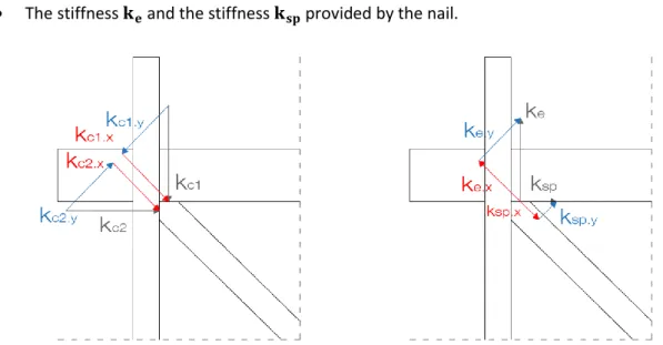
Following the procedure presented previously, the component method is applied to calculate the axial and shear stiffness of the connections between the diagonal elements and the main frame. As shown in Figure 4, the following stiffness are considered:

 The stiffness provided by the contact areas;

 The stiffness and the stiffness provided by the nail.

Figure 4. Axial and shear stiffness for the connection between the diagonals and the main frame.

Considering the stiffness by contact , two contact areas, 1 and , are identified for each

connection as shown in Figure 5. In turns, the compression stiffness is calculated for the –

couple of surfaces in contact , by considering their elastic stiffness, 1 and . Each elastic

stiffness was evaluated by applying ( 4 ) and considering the slope of grain of each timber element: = 1.66 106 kN/m2 (α = 45°) and = 9 105 kN/m2 are the moduli of elasticity considered for the

(32)

Finally, the axial stiffness and shear stiffness in compression are calculated considering the

projection of the elastic stiffness for the –couple of surfaces, and . The obtained values

are summarized in Table 3.

Figure 5. Contact areas of the connections by contact. Table 3. Axial and shear stiffness for the connection by contact.

A1 [m2] kc11 [kN/m] kc12 [kN/m] kc1 [kN/m] kc1.x [kN/m] kc1.y [kN/m] 6.84∙10–4 1.15∙105 6.20∙104 4.02∙104 2.85∙104 2.85∙104 A2 [m2] kc21 [kN/m] kc22 [kN/m] kc2 [kN/m] kc2.x [kN/m] kc2.y [kN/m] 6.84∙10–4 1.15∙105 6.20∙104 4.02∙104 2.85∙104 2.85∙104

As shown in Figure 4, two contributions are considered to estimate the stiffness of the nail: (1) the extraction stiffness and (2)the ultimate shear plane stiffness .The extraction stiffness can

be calculated by considering the axial strain of a linear elastic isotropic material, as follows

where = 210 GPa is the modulus of elasticity of steel, = 28.27 mm2 is the cross sectional area of the nail and n = 7 cm is the penetration length. In particular, the penetration length is calculated as

the length of the nail piercing the timber element excluding the possible gap present in the connection.

Concerning the ultimate shear plane stiffness , the formula provided by Eurocode 5 (2004) for

nails without pre–drilling is used:

n

(33)

where = 590 kg/m3 is the mean density of the wood and = 6 mm is the diameter of the nail. Hence, by considering the projections of the stiffness values found, the axial and the shear stiffness are calculated on the parallel and perpendicular directions. The values obtained are summarized in Table 4. However, the value calculated for the nail that results to be pushed–out from the connection seems to be rather high.

Table 4. Axial and shear stiffness for the connection by contact. [kN/m] [kN/m] [kN/m] [kN/m] [kN/m] [kN/m] 8.48 ∙ 104 6 ∙ 104 6 ∙ 104 1.34 ∙ 103 944 944

2.3.3 Evaluation of the rotational stiffness

The component method presented in Section 3.2.1 is applied to calculate the elastic rotational stiffness of the half–lap connections between the elements of the main frame. As shown in Figure 6, four contact areas are identified and the corresponding elastic stiffness values are calculated taking into account the slope of grain. If is the applied bending moment and is the relative rotation between the connected members, the rotational stiffness of the half–lap joints can be written as (Descamps & Guerlement, 2009):

where is the elastic stiffness of each –couple of surfaces and is the distance between the point of application of each stiffness and the instantaneous centre of rotation (ICR). In this case, the ICR is assumed to be fixed and located where the nail of the half–lap joint is placed. Enhancement of the ICR definition is provided by Descamps (2009) considering its movement during loading. The value of 477 kNm/rad can be assumed for the rotational stiffness . A summary of

the obtained results is shown in Table 5. [ 1 ] ( 7 ) ∑ ∑ ∑ ∑ ( 8 )

(34)

Table 5. Rotational stiffness for the half–lap connection. A1 [m2] k11 [kN/m] k12 [kN/m] k1 [kN/m] z1 [m] 9.60 ∙ 10–3 1.04 ∙ 106 7.84 ∙ 104 1.15 ∙ 104 0.05 A3 [m2] k31 [kN/m] k32 [kN/m] k3 [kN/m] z3 [m] 6.80 ∙ 10–4 5.18 ∙ 105 4.24 ∙ 104 3.92 ∙ 104 0.02

(35)

2.4 Numerical model

In order to simulate the mechanical behaviour that was observed for the pre–compression load of 25 kN in the experimental testsdescribed in Section 2.2, the timber frame wall is modelled by using

Frame and Link elements in SAP2000 structural and earthquake engineering software.The calibration of the model is performed by comparing the numerical and the experimental capacity curves. It should to be noted that only the positive values of the experimental diagram are taken into account. This is due to the fact that the load was applied only on one side during testing and this provoked an asymmetrical response.

2.4.1 Geometry and material properties

Timber is modelled as a linear elastic isotropic homogeneous material. According to the experimental results, the value of the modulus of elasticity is 1 ∙ 107 KN/m2 and the Poisson’s ratio is 0.3. Geometrically, the model consists of four cells that are assumed to have the same dimensions of 0.95 x 0.95 m2, as shown in Figure 7.

Figure 7. Schematic of the numerical model.

Figure 8 presents four different models that depend on the assumptions made for the timber

connections:

 MOD 0 : Rigid connection for each joint;

 MOD 1 : Hinged connection between the diagonal elements and the main frame;

(36)

 MOD 3 : Semi–rigid connections between (1) the diagonal elements and the main frame,

and (2) the elements of the main frame.

Figure 8. Typical cell for each numerical model.

It should be noted that the half-lap connections in the diagonals are not modelled, as it was observed during the experimental campaign that they have little influence on the behaviour of the wall (Poletti, 2013). Each element of the main frame is modelled as Frame element – a straight line connecting two points. In order to model the semi–rigid connection, Link element – two joint connecting link – is used with multi–linear elasticity property. Each link element is assumed to be composed of six separate springs, one for each deformational degree of freedom. The link element is assumed to have zero length. This is performed by setting the distance between the two connected joints as the value in the Auto Merge Tolerance. The Advanced local coordinate system is used to define the orientation of local 1 axis coincident with the longitudinal axis of the element that is connected to the link element. For the link element deformational degree of freedom (DOF), three options are available:

 Option unchecked: any contributing stiffness is kept to the direction specified for the link;

 Fixed option: the link does not experience any deformation in the direction specified;

 Nonlinear option: the link contributes the specified stiffness.

It is possible to fix either all or none of the link element deformational DOF. However, link elements with fixed element deformational DOFs should not be connected to constrained joints as these might result to be multiply–constrained. As it will be described in the following sections, the left corner of

(37)

the top beam needs to be restrained in order to apply a horizontal displacement. Moreover, the link elements that will be used are present at the same location. For this reason, it is necessary that all the element deformational DOFs are not fixed. Reasonable large stiffness values are considered in order to specify a stiff behaviour, as recommended by CSI (2014).

For each internal deformation – that does not affect the behaviour of any other – a multi–linear elastic force–deformation relationship can be specified. A multi–linear curve can be defined by a set of points respecting some restrictions given by CSI (2014) in order to describe a nonlinear elastic behaviour for the timber connections.

In this study, two link elements are considered: Link 1 and Link 2. Link 1 is located at each connection between the main frame and the diagonal elements in MOD 2 and MOD 3. In MOD 3, Link 2 is located at each beam–post connection. Because of the planar nature of the problem, only the axial

1, shear and pure bending stiffness are considered for the element deformational DOFs. While

the axial and the shear stiffness are specified for Link 1, the rotational one is defined for Link 2. Linear elastic force–deformation relationships are used for Link 1 in MOD 2 (Figure 9); linear and nonlinear elastic force–deformation ones are introduced for Link 1 and Link 2 in MOD 3 (Figure 10).

(38)

Figure 10. Linear and nonlinear elastic force–deformation for Link 1 and Link 2 in MOD 3.

2.4.2 Loading condition

In order to simulate the experimental tests described in Section 2.2, the following load conditions are considered for the model of the timber frame wall:

 Vertical load of 25 kN applied downwards at the three nodes intersecting the top beam and

the posts;

 Horizontal displacement of 0.10 m applied on the left corner of the top beam. 2.4.3 Restraints

For the full wall, as shown next, the three nodes of the bottom beam are restrained in the vertical and horizontal directions. Besides, the left corner of the top beam is restrained in the horizontal

(39)

direction in order to apply the prescribed displacement. In MOD 1, all the rotational DOFs of each diagonal element are released at one end in in order to model the connection as a hinge.

2.4.4 Structural analysis

In order to obtain the capacity curve of the structural system, the following two steps of a nonlinear static analysis are performed:

 Full load application of the dead and vertical loads;

 Displacement control of the applied horizontal displacement.

The capacity curve is constructed by considering the base shear and the applied horizontal displacement at each step of the nonlinear analysis. As expected, when no non–linearity is present in the model in terms of geometry, material, loading and boundary condition – such as in MOD 0, MOD 1 and MOD 2 – the results are the same of those obtained by performing a linear static analysis. Nonlinearity is only introduced in MOD 3, considering the capacity for both timber connections under study.

2.5 Calibration of the model

As explained in Section 2.2.5, the secant stiffness of the timber wall was calculated and a value of 2.60 ∙ 103 kN/m was obtained for the lower pre–compression load. In order to calibrate the numerical model, the following study was performed considering the four different models described in Section 2.4.1.

2.5.1 Model with rigid connections (MOD 0)

Firstly, MOD 0 is considered with rigid connections for all joints. By observing the deformed shape in

Figure 11, it is noted that the deformation is mostly due to the application of the horizontal

displacements. Moreover, all the nodes behave rigidly as expected. As observed in the axial forces diagram, the diagonal elements that are inclined along (against) the applied displacement are in tension (compression). The value of the stiffness of the timber frame wall is 39.94 ∙ 103 kN/m, which is much higher than the experimental value.

(40)

Figure 11. Deformed shape (left) and axial force diagram (right) of MOD 0.

2.5.2 Model with hinged connections of the diagonal elements (MOD 1)

In MOD 1, all the diagonal elements are released at one end in all the rotational DOFs. The value of the stiffness obtained is 39.87 ∙ 103 kN/m. As this is slightly lower than that obtained in MOD 0, the rotational stiffness between the diagonals and the main frame appears not to be significant, which is expected in timber structures due to the low bending stiffness and the almost rigid triangular configuration of the structure. By eliminating one of the diagonal elements for each cell of the wall, the stiffness of the structure is 22.17 ∙103_{kN/m, almost the half of the original value (MOD 1_BIS).} This is also expected because, elastically, all diagonals work similarly, independently of the connection being in tension or compression.

2.5.3 Model with semi–rigid connections of the diagonal elements (MOD 2)

In order to provide more flexibility in MOD 2, all the connections between the diagonal elements and the main frame are modelled as Link 1 described in Section 2.4.1. In particular,the axial and shear deformational DOFs of Link 1 are modelled with a linear elastic force–deformation relationship. Let 1 and 1+be the axial stiffness of Link 1 in compression and in tension, respectively (Figure 10). By assuming 1 1+ and applying the inverse fitting method, the stiffness of the structure reaches the experimental value when the stiffness of the connection results to be 1 1+ = 4.15 ∙ 103 kN/m. In particular, an almost linear relationship is observed between the stiffness of the connection and that of the structure. This confirms that the rotational stiffness of the connection between the diagonals and the main frame appears to be negligible. Assuming 1 = 4.15 ∙ 103 kN/m and 1+ = 0 kN/m - and vice versa – the value of the stiffness of the structure is halved. This is equivalent to

(41)

removing one diagonal element – and all its link elements – for each cell of the wall, as shown in MOD 2_O. Moreover, taking the value of the stiffness in compression as the double of the previous one and zero stiffness in tension, as shown in MOD 2_A, the value of the stiffness of the structure is slightly lower than the experimental one. The exact experimental value is reached by considering the stiffness in tension of the connection as 1+ 1 in MOD 2_B. Note that the shear stiffness does not seem to affect the result when linear elastic properties are applied, as shown by comparing MOD_2_A with MOD_2_C in Table 6.

Table 6. Results of the numerical model MOD 2.

MOD 2 MOD 2_0 MOD_2_A MOD 2_B MOD 2_C

LINK 1 1 1+ [KN/m] 1 [KN/m] 4.15∙103 4.15∙103 0 4.15∙103 0 8.50∙103 85 8.50∙103 0 8.50∙103 + [KN/m] [KN/m] ∞ ∞ ∞ ∞ ∞ ∞ ∞ ∞ 8.50∙103 8.50∙103 + [KNm/rad] [KNm/rad] 0 0 0 0 0 0 0 0 0 0 Global stiffness K [kN/m] 2.60∙103 1.65∙103 2.58∙103 2.60∙103 2.58∙103

2.5.4 Model with semi–rigid connections of the diagonal elements and elements of the main frame (MOD 3)

As previously explained, Link 1 and Link 2 are used in MOD 3: while the axial 1 and the shear

stiffness are specified for the former, the rotational one is defined for the latter. Initially, linear elastic force–deformation relationships are considered for the link elements. The results on in–plane cyclic tests on half-lap joints with a pre–compression vertical load of 25 kN obtained by Poletti (2013) are used to define the deformational DOF of Link 2. The average force–displacement diagram is calculated from the experimental curves and a tri–linear curve is assumed for the numerical model, as shown in Figure 12. The corresponding tri–linear moment–rotation diagram shown in Figure 13 is obtained. The mean values of the initial and the final rotational stiffness are calculated as in = 171

kNm/rad and in = 47 kNm/rad, respectively.

As the axial stiffness of Link 1 in tension is not influencing the structural behaviour significantly, it is assumed to be zero. By applying the inverse fitting method, the axial stiffness of the connection in compression is calculated as 10 ∙ 103 kN/m (MOD 3_A). By assuming the axial stiffness in tension of the connection as 1+ 1 (MOD 3_B), the value of the stiffness is 2.56 ∙ 103 kN/m, slightly lower than the experimental one. Finally, it is noticeable that the shear stiffness does not seem to

(42)

affect the result when linear elastic properties are applied (MOD 3_C). A summary of all the results is presented in Table 7.

Figure 12. Force–displacement for the half–lap connection.

Figure 13. Moment–rotation for the half–lap connection. Table 7. Results of the linear elastic analysis on MOD 3.

MOD 3_A MOD 3_B MOD 3_C

LINK 1 1 1+ [KN/m] 1 [KN/m] 0 10∙103 100 10∙103 0 10∙103 + [KN/m] [KN/m] ∞ ∞ ∞ ∞ 10∙103 10∙103 + = [KNm/rad] 0 0 0 LINK 2 1 1+ = 1 [KN/m] ∞ ∞ ∞ + = [KN/m] ∞ ∞ ∞ in + = in [kNm/rad] in + = in [kNm/rad] 171 47 171 47 171 47 Global Stiffness K [kN/m] 2.53∙103 2.56∙103 2.56∙103 in in

(43)

Subsequently, nonlinear elastic force–deformation relationships are introduced by considering the capacity of the two timber connections, as shown in Figure 10. The tri–linear moment–rotation diagram described previously is used to define the multi–linear curve for the deformational DOF of

Link 2. An initial linear behaviour followed by a linear softening is considered as the multi–linear

curve to define the axial and shear deformational DOFs of Link 1. The capacity of the connection is calculated by considering the compressive strength perpendicular to the grain and the contact

areas for each connection by applying ( 9 ). In particular, only one contact area is considered due to the presence of initial clearances and the development of damage during the experimental tests. Hence, also the yield displacement needs to be defined by applying ( 10 ).

The ultimate displacement is assumed to be the same of that of half–lap connections: when the failure occurs for the half–lap connection, the connection between the diagonal and the main frame no longer works. When the ultimate displacement is reached ( = 50 mm), the capacity of the connection between the diagonals and the main frame is assumed to be zero ( = 0 kN). This is assumed for both the axial and shear stiffness of Link 1.

Due to the absence of experimental tests, parametric analyses have been carried out to better understand the influence of the capacity and of the stiffness of the connection between the diagonals and the main frame on the timber frame wall, as shown in Table 8. Different compressive strength values perpendicular to the grain are considered as this value was not directly derived from experimental tests described in previous section and it can vary greatly. Hence, different capacity values are considered. As shown in Figure 14, changing the compressive strength perpendicular to the grain affects mostly the initial behaviour. For a fixed value of the connection stiffness, an

increase in the compressive strength leads to higher values of capacity and of yield displacement of the timber frame wall, as expected. As the displacement increases, the effect fades out. Considering the value of = 5 MPa (

Table 2) – that corresponds to a capacity value of 23.9 kN – C_1 reaches a capacity of less than 4kN.

The capacity value obtained considering C_5 ( = 6 MPa) can be assumed to approximate

reasonably well the experimental curve. On the other hand, changing the stiffness affects significantly the initial stiffness of the structure, while the capacity changes slightly, as shown in

⁄

( 9 ) ( 10 )

(44)

Figure 15. The value obtained previously by applying the inverse fitting method in the elastic analysis

is assumed as the initial stiffness of the connection between the diagonal and the main frame.

Table 8. Parametric analysis on the connection between the diagonals and the main frame.

CAPACITY STIFFNESS C_1 C_2 C_3 C_4 C_5 S_4 S_5 S_6 LINK 1 u1 1+[KN/m] 1 [KN/m] [KN] 0 10000 23.9 0 10000 25.7 0 10000 27.4 0 10000 29.1 0 10000 30.8 0 10000 30.8 0 20000 30.8 0 50000 30.8 u2 + = [KN/m] [KN] 10000 23.9 10000 25.7 10000 27.4 10000 29.1 10000 30.8 10000 30.8 20000 30.8 50000 30.8 r3 + = [KNm/rad] 0 0 0 0 0 0 0 0 LINK 2 u1 1+= 1 [KN/m] ∞ ∞ ∞ ∞ ∞ ∞ ∞ ∞ u2 + = [KN/m] ∞ ∞ ∞ ∞ ∞ ∞ ∞ ∞ r3 in + = in [kNm/rad] in + = in [kNm/rad] 171 47 171 47 171 47 171 47 171 47 171 47 171 47 171 47

Figure 14. Parametric analysis on the capacity of the connection between the diagonals and the main frame.

(45)

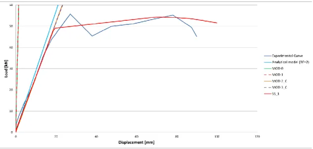
Differently from the results obtained using linear elastic analysis, the shear stiffness has influence on the nonlinear structural behaviour. While the compressive strength value perpendicular to the grain and the axial stiffness influence mainly the initial behaviour, the shear stiffness seems to affect mostly the nonlinear response of the timber frame wall, as shown in Table 9 and Figure 16. It should be noted that the curves obtained from MOD SS_1 and MOD SS_2 are very similar, while a marked softening is experienced by SS_3 – that corresponds to having only axial forces in the diagonal elements of the timber frame wall. The influence of the positive and negative shear stiffness is studied independently in SS_4 and SS_5.

Table 9. Influence of shear stiffness in nonlinear analysis.

SS_1 SS_2 SS_3 SS_4 SS_5 SS_6 SS_7 SS_8 LINK 1 u1 1+[KN/m] 1 [KN/m] [KN] 0 10000 30.8 0 10000 30.8 0 10000 30.8 0 10000 30.8 0 10000 30.8 0 10000 30.8 0 10000 30.8 0 10000 30.8 u2 + [kN/m] [kN] [kN/m] [kN] 10000 30.8 10000 30.8 ∞ ∞ ∞ ∞ 0 0 0 0 0 0 10000 30.8 10000 30.8 0 0 10000 15.4 10000 15.4 5000 30.8 5000 30.8 5000 15.4 5000 15.4 r3 + = [kNm/rad] 0 0 0 0 0 0 0 0 LINK 2 u1 1+= 1 [KN/m] ∞ ∞ ∞ ∞ ∞ ∞ ∞ ∞ u2 + = [kN/m] ∞ ∞ ∞ ∞ ∞ ∞ ∞ ∞ r3 in + = in [kNm/rad] in + = in [kNm/rad] 171 47 171 47 171 47 171 47 171 47 171 47 171 47 171 47

(46)

Figure 17. Influence of the shear stiffness.

2.6 Conclusion

In order to simulate the mechanical behaviour that was observed during the quasi–static in–plane cyclic tests carried out by Poletti (2013), analytical and numerical modelling of the timber wall were carried out.

Firstly, the analytical model of the timber joints was constructed by applying the component method. In particular, the axial and shear stiffness were computed for the connection between the diagonal elements and the main frame, while the rotational stiffness was evaluated for the half–lap connections of the main frame. Two main contributions to the stiffness were evaluated to obtain the axial and shear stiffness: the stiffness due to the contact areas between the wooden elements and the one provided by the nail. It should be noted that the evaluation of the axial stiffness in tension was a difficult task. While the shape of deformed nails confirmed the plane shear contribution – even though it was not so significant – not much information was available regarding their elongation. Hence, the evaluation of stiffness based on the elastic strain was performed and a very high value was obtained. Regarding the rotational stiffness of the half–lap joint, only the stiffness due to the contact areas between the corresponding wooden elements were considered. A summary of the obtained values is shown in Table 10.