SPATIAL VARIABILITY OF SOYBEAN YIELD THROUGH A REPARAMETERIZED T- STUDENT MODEL

Engineering

ISSN: 1809-4430 (on-line)

_________________________ 1

Centro de Ciências Exatas e Tecnológica, Universidade Estadual do Oeste do Paraná - UNIOESTE/ Cascavel - PR, Brasil. 3 _{Departamento de Estadística, Pontificia Universidad Católica de Chile/ Santiago, Chile.}

4

COMAT, Universidade Tecnológica Federal do Paraná/ UTFPR/ Toledo - PR, Brasil. Received in: 4-28-2016

SPATIAL VARIABILITY OF SOYBEAN YIELD THROUGH A REPARAMETERIZED T-STUDENT MODEL

Doi:http://dx.doi.org/10.1590/1809-4430-Eng.Agric.v37n4p760-770/2017

ROSANGELA C. SCHEMMER1, MIGUEL A. URIBE-OPAZO2*, MANUEL GALEA3, ROSANGELA A. B. ASSUMPÇÃO4

2*

Corresponding author. Centro de Ciências Exatas e Tecnológica, Universidade Estadual do Oeste do Paraná - UNIOESTE/ Cascavel - PR, Brasil. E-mail: miguel.opazo@unioeste.br

ABSTRACT: The t-Student distribution has been used to the spatial dependence modelling of soybean yield as an alternative to the normal distribution, being used for data with heavier tails or discrepant values. However, a usual Student t-distribution does not allow direct comparisons of geostatistical methods with a normal distribution. The aim of this study was to assess the soybean yield spatial variability through a reparameterized t-Student linear model, comparing the results with those of a Gaussian linear model. For parameter estimation, a complete maximum likelihood (CML) method was used through an expectation-maximization (EM) algorithm. The maps constructed with both reparameterized t-Student and normal distributions are dissimilar and present a kappa index (K) equivalent to 0.64. The reparameterized t-Student distribution is an alternative in studying data with discrepant values, showing the ability to decrease the influence of these points.

KEYWORDS: EM algorithm, spatial dependence, geostatistics, complete maximum likelihood.

INTRODUCTION

Geostatistics can assist in precision agriculture since its techniques allow constructing maps that determine the spatial dependence structure of yield associated with soil and plant attributes. Thus, it helps the producer to decide on the use of agricultural inputs in appropriate quantities and locations in order to increase yield, reduce losses, and maintain environmental quality. This technique is based on the regionalized variable theory proposed by Matheron, influenced by the observations made by Kriger. According to Vieira (2000), Kriger analyzed gold concentration data in South Africa and observed the impossibility of finding meaning in the variances without taking into account the distance between samples. Therefore, the values of a variable distributed in the space are correlated within a radius of spatial dependence.

This study aimed to assess the spatial variability of soybean yield by means of a reparameterized t-Student linear model, comparing the results with a Gaussian linear model. For estimating these model parameters, a complete maximum likelihood (CML) method was used through an expectation-maximization (EM) algorithm.

THEORETICAL FOUNDATION Reparameterized t-Student distribution

Much of the statistical inference involving continuous random variables is based on normal distribution. However, to obtain reasonable inferences, assuming normality, it is necessary to ensure conditions such as symmetry and a certain value of kurtosis. Among the symmetric models alternative to the normal distribution is the t-Student distribution, which presents as an additional parameter the degree of freedom v v



0



that allows kurtosis modeling. A priori, this parameter can be fixed. However, Lange et al. (1989) recommend fixing it at v4 for a small data set and its estimation for a large data set. This distribution has been widely used in the study with real data because it has tails longer than the normal distribution and allows the discrepant points present in the data set to be encompassed (Lange et al., 1989; Osorio et al., 2007). Galea et al. (2002) suggest the t-Student distribution as an alternative to the normal distribution due to the statistical inference based on the t-Student distribution to combine conceptual and computational simplicity with generality, in addition to being applicable in a great variety of situations. An important feature of t-Student distribution is that when the degree of freedom v increases, the t-Student distribution approaches to the normal probability distribution.

Lange et al. (1989) state that if a random vector Y



Y₁, ,Y_n



T has as probability density function multivariate t-Student with a location parameter μ, scale matrixV, and v0 degrees of freedom, Y t_n



μ1 V, ,v



is denoted. The expectation of the random vector Y is E

 

Y μ1, where 1 is a vector of 1’s of order n × 1, for v1, and the covariance matrix n × n of Y is

 

2

v v

Cov  

 V

Y Σ for v2. For values of v2, the covariance matrix Cov

 

Y is undefined.

Lange et al. (1989) suggest the reparametrization of t-Student distribution for allowing the direct comparison between parameter estimation of the mean vector and the covariance matrix with the model assuming normality. The authors also mention that an improvement of inference is observed when the degree of freedom presents the transformation v1 .





1, ,



T n

Y Y



Y is considered a random vector that has reparameterized t-Student distribution with shape parameter  fixed, in which 0 1 ,

2



  with covariance matrixΣ, mean vector

 

E Y μ1 if its probability density function is given by [eq. (1)]:

 

 

1

 

1₁ 

2 ₂

2 1 ,

n n

f_Y y K  Σ _ c   _   (1) where,

 

 

2

1 2 , 1 2 n n n c K              _{ }    _{ }   _{ }  

Which



2 



Yμ1



T Σ Y 11



μ



is the Mahalanobis distance, c( )

 





1 2





and 0 1 . 2



It is denoted by Y



_n



μ1, ,Σ





that the vector Y has n-variate reparameterized t-Student distribution.

Spatial linear model

For the study of spatial dependence,



Y s( ),_i s_iS



is considered a stochastic process of second-order stationary, where S 2 and 2 is a two-dimensional Euclidean space. Let



( ),1 , ( )



T n

Y s Y s



Y be a vector n × 1 of the response variable corresponding to spatial locations known in si with i= 1, …, n. The georeferenced variable Y s( )i can be written as:

Y s( )_i 



( )s_i e s( ),_i (2) being the deterministic term



( )s_i  x_iTβ, where xT_i 



x_i1, ,x_ip



is a vector 1 × p of explanatory variables at position s_i, β



₁, ,_p



Tis the vector p × 1 of unknown parameters to be estimated, and e s( )_i is a spatially correlated random component.

Equation (2) can be written in a matrix form as:

,

 

Y Xβ

ε

(3)

where X is a matrix n×p of columns with complete rank, with lines xTi and



( ),1 , ( )



,

T n

e s e s



ε

with i = 1, …, n. It is assumed that the random errors e s( )_i have zero mean, i.e. E e s



( )_i



0 and the variation between points in space is determined by some covariance function



( ), ( )_{i u}





Y( ), Y( )_{i u}





_i, _u



_iu

Cov e s e s Cov s s C s s 



for i, u = 1, …, n. The spatial modeling given in [eq. (3)] depends on the covariance matrix structure Σ _

 



_iu _, where



_iu=C s s



_i, _u



for i,u =

1, …, n, of the stochastic process Y. The covariance function C s s



_i, _u



is used in the study of spatial dependence of the stationary process and it is specified by a three-dimensional vector



1, 2, 3



T

  



φ of the form given in [eq. (4)] (Uribe-Opazo et al., 2012):

Σ₁I_n₂R (4) where₁is the parameter nugget effect





₁0 ,



₂ is the parameter sill





₂0 ,



R is a symmetric matrix n×n, whose elements are as a function of the parameter





₃ 0





R R

   

₃  _ r_iu _



with diagonal elements r_ii 1 and r_iu 



₂1C s s



_i, _u



for  ₂ 0and r_iu 0 for  ₂ 0, i ≠ u = 1, …, n, being r_iudependent on the Euclidian distance h_iu  s_is_u between the points s_iand s_u, and I_nis the identity matrix n × n. The parametric form of the covariance matrix Σ, represented in [eq. (4)], occurs for several stationary and isotropic processes, in which the covariance C s s



_i, _u



C h

 

_iu is defined by the covariance function C h

 

_iu 



₂r_iu. In the covariance functions C h

 

_iu , the variance of the stochastic process reparameterized t-Student Y is given by C

 

0  

 

_{1 2}.

On the assumption that Y



_n



Xβ Σ, ,





, where  represents the shape parameter, considered fixed and the unknown parameters of the model θ β φ



T, T



T, with



1, ,



T p

 



β

function defined by [eq. (5)]:

 

ˆ_{, max}





_,





_,

c c c c

l θ Y  l θ Y (5) being





_{ }

 

_{ }

 

2

1 1 1 1

, log(2 ) log log

2 2 2 2 2

1 1

log log log ,

2 2 2

c c n l c c       _{  }          _{ }       __{ }  _  _    

θ Y Σ

(6)

where



2 



Y X β Σ Y Xβ



T 1







, c( )

 





1 2





,



0 and 0  1₂.

Maximization of [eq. (6)] is obtained by using an iterative process. In this case, the EM (expectation and maximization) algorithm was applied, being the stopping criterion the relative error (RE), where RE ,

r ( r - 1) r

r

-

= θ θ 

θ with

5

10

 . To determine the shape parameter 

considered fixed, the criteria of cross-validation



VC

 





, presented by De Bastiani et al. (2015), and the trace criterion



T_r

 





, proposed by Kano et al. (1993), were applied. For the reparameterized t-Student model, cross-validation is given by [eq. (7)]:

2 1 ˆ ( ) ( ) 1 ( ) , 1 n

i i i

i ii

y s y s

VC n h    _{  }     _{ }      



 (7)

where y sˆ_i( )_i x_iTβˆ_i, with x_iT 



x_i1, ,x_ip



being the i-th line of the matrix X, is the prediction at the location s_i without considering the observation



y_i,x_iT



, βˆ_i is the maximum likelihood estimator for _i without considering the i-th observation and h_ii is the i-th diagonal element of the matrix Hat (





1

1 1

ˆ ˆ

T   T  

H X X Σ X X Σ ), also called a projection matrix. Trace criterion consists of calculating the trace of the asymptotic covariance matrix of the estimated mean



μ Xβˆ  ˆ



, as a criterion in choosing considering that the shape parameter is obtained by:













_

_

_

_

1

1

1 2 1 2 _ˆ

( ) , 1 T T r n T tr n            _{ }  _{    }  

  X X X Σ X

(8)

Where Σˆ 



ˆ₁I_n



ˆ₂Rˆ. For the two criteria, the best shape parameter  is determined by the lowest values of cross-validation



VC

 





and trace



Tr

 





. After choosing the estimation of , the best

 





 





*

1 1

2 *

1

,

r r

ii i i i i

r

i i i

N n n n

K

N n n

 

 

  

 









(9)

where N* is the total area, nii is the area belonging to class i of the model and reference maps, ni+ is

the area belonging to class i of the model map, n+i is the area belonging to class i of the reference

map, and r is the number of classes. According to Krippendorff (2004) classification, K is classified with low similarity if K < 0.67, medium similarity if 0.67 < K < 0.80, and high similarity if K > 0.80.

MATERIAL AND METHODS

Location and characteristics of the study area

Data on soybean yield, plant height, and pods per plant were collected from an experimental area of 47.95 ha located in Cascavel, the western region of Paraná, Brazil, with an approximate location of 24.83° S and 53.60° W, and an average altitude of 650 meters. The soil of this area is classified as a clayey Oxisol (Haplorthox) (EMBRAPA, 2011) and regional climate is a temperate super-humid climate type Cfa (Köeppen) with average annual temperature of 21 °C. All samples were georeferenced in the spatial coordinate system (UTM) by using a Trimble GPS25 (Global Positioning System) GEOEXPLORER 3 data receiver. Figure 1 shows the experimental area in a regular grid of 75 × 75 meters, totaling 83 observations for the 2006/2007 agricultural season.

FIGURE 1. Area location in the 2006/2007 agricultural season.

Statistical analyses were performed using the free software R, version 3.2.0 (R Core Team, 2016). The following packages were used: geoR (Ribeiro Junior & Diggle, 2016) for studying the spatial data, map construction by regression kriging interpolation, and comparison of thematic maps; matrixcalc (Novomestky, 2012) for trace calculation; e1071 (Meyer et al., 2015) for calculating the asymmetry and kurtosis; and classInt (Bivand, 2015) for choosing the class intervals for continuous numerical variables.

RESULTS AND DISCUSSION

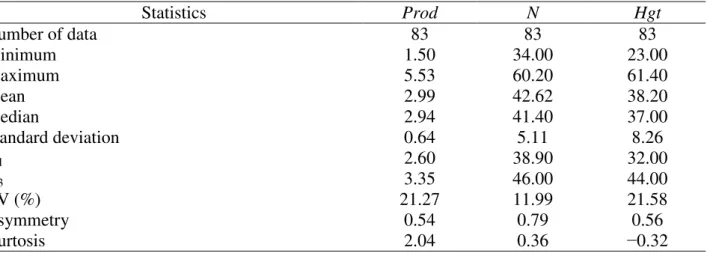
Table 1 shows the exploratory analysis of values found for the variables soybean yield (Prod) (t ha−1), average plant height (Hgt) (cm), and an average number of pods (N). The average soybean yield is 2.99 t ha−1, with a minimum value of 1.50 t ha−1 and a maximum value of 5.53 t ha−1. Moreover, 75% of the area presents a yield lower than or equal to 3.35 t ha−1. Soybean yield is classified as heterogeneous since the coefficient of variation (CV) is 21.27%.

TABLE 1. Descriptive statistics for the variable soybean yield (Prod), the covariates average plant height (Hgt) and an average number of pods (N).

Statistics Prod N Hgt

Number of data 83 83 83

Minimum 1.50 34.00 23.00

Maximum 5.53 60.20 61.40

Mean 2.99 42.62 38.20

Median 2.94 41.40 37.00

Standard deviation 0.64 5.11 8.26

Q1 2.60 38.90 32.00

Q3 3.35 46.00 44.00

CV (%) 21.27 11.99 21.58

Asymmetry 0.54 0.79 0.56

Kurtosis 2.04 0.36 −0.32

Q1: 1st quartile; Q3: 3rd quartile; CV: coefficient of variation.

The boxplot graph presented in Figure 2a detected a single discrepant point, which corresponds to the sample element 6, with coordinates (236325, 7250475), referring to the maximum yield value in the data set, being equivalent to 5.53 t ha−1. According to the Postplot graph shown in Figure 2b, observation 6 is in a region where the nearest neighbors have a soybean yield between 2.60 and 2.94 t ha−1.

In order to identify the spatial dependence structure of soybean yield as a function of the average plant height (Hgt) and an average number of pods per plant (N), the average soybean yield

 

si



in the position s_i  S 2 was considered as a spatial linear regression model given by:

1 2 3

( )s_i Hgt s( )_i N s( ),_i i 1, , ,n

     (10) where  1, 2, and 3 are the unknown parameters to be estimated.

Parameter estimation studies were performed by complete maximum likelihood (CML) using the EM algorithm of the spatial linear model defined in [eq. (10)] and parameters of the spatial dependence structure Σ given in [eq. (4)], considering the Matérn family with parameters



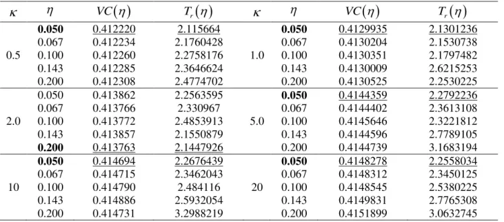
0.5, 1.0, 2.0, 5.0, 10 and 20 associated to shape parameters of the reparameterized t-Student   0.05, 0.067, 0.1, 0.143, and 0.2.

Table 2 shows the determination of the best shape parameter  of the reparameterized t-Student distribution associated to each shape parameter



of the Matérn family using the cross-validation criterion and trace defined by Equations (7) and (8). In bold is presented the choice of each parameter  for each



with the lowest values of cross-validation



VC

 





and trace

 



Tr 



.

TABLE2. Cross-validation and trace for the choice of the best shape parameter .



 VC

 

 T_r

 





 VC

 

 T_r

 



0.050 0.412220 2.115664 0.050 0.4129935 2.1301236

0.067 0.412234 2.1760428 0.067 0.4130204 2.1530738

0.5 0.100 0.412260 2.2758176 1.0 0.100 0.4130351 2.1797482

0.143 0.412285 2.3646624 0.143 0.4130009 2.6215253

0.200 0.412308 2.4774702 0.200 0.4130525 2.2530225

0.050 0.413862 2.2563595 0.050 0.4144359 2.2792236

0.067 0.413766 2.330967 0.067 0.4144402 2.3613108

2.0 0.100 0.413772 2.4853913 5.0 0.100 0.4145646 2.3221812

0.143 0.413857 2.1550879 0.143 0.4144596 2.7789105

0.200 0.413763 2.1447926 0.200 0.4144739 3.1683194

0.050 0.414694 2.2676439 0.050 0.4148278 2.2558034

0.067 0.414715 2.3462043 0.067 0.4148312 2.3450125

10 0.100 0.414790 2.484116 20 0.100 0.4148545 2.5380225

0.143 0.414886 2.5932054 0.143 0.4149831 2.7765308

0.200 0.414731 3.2988219 0.200 0.4151899 3.0632745

: shape parameter; VC

 

 : cross-validation; _Tr

 

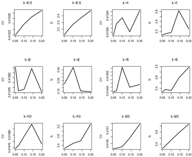
 : trace; : shape parameter of the Matérn family. In bold is the best shape parameter ; underlined is the lowest value of cross-validation and trace.

Figure 3 shows the cross-validation VC

 

 and trace T_r

 

 graphs for each



value of the Matérn family model related to those chosen in Table 3. For



0.5 and 20, VC

 

 and T_r

 



values increase as  value increases. For the other cases, when  values increase, VC

 

 and

 

r

FIGURE 3.Graphs of cross-validation VC

 

 and trace Tr

 

 .

Table 3 shows the results of parameter estimation and the respective standard deviations considering the  values for each



selected in Table 2. The lowest standard deviations of estimators correspond to the estimated values of  0.050 and 0.5, whose estimates are ˆ₁ = 0.993, ˆ₂ = 0.021, ˆ₃ = 0.030, ˆ₁ = 0.248, ˆ₂ = 0.121, and ˆ₃ = 112.8, with a practical range of approximately 338.0 m.

TABLE 3. Estimation of the parameters and  via EM algorithm for different and .



1

ˆ

 ˆ₂ ˆ₃ ˆ1 ˆ2 ˆ3

0.5 0.050 0.993 0.021 0.030 0.248 0.121 112.8

(0.7216) (0.0144) (0.0077) (0.1189) (0.8792) (0.0003)

1.0 0.050 0.978 0.022 0.030 0.270 0.087 96.88

(0.7319) (0.0146) (0.0080) (0.1141) (0.8905) (0.0003)

2.0 0.200 0.965 0.022 0.030 0.273 0.072 76.69

(0.7433) (0.0148) (0.0080) (0.3028) (1.6411) (0.0005)

5.0 0.050 0.959 0.022 0.031 0.300 0.072 49.09

(0.7478) (0.0149) (0.0080) (0.1214) (0.9141) (0.0002)

10 0.050 0.956 0.022 0.031 0.302 0.070 34.68

(0.7483) (0.0149) (0.0080) (0.1219) (0.9190) (0.0003)

20 0.050 0.956 0.022 0.031 0.303 0.069 24.39

(0.7489) (0.0148) (0.0080) (0.1223) (0.9216) (0.0005)

. ˆ

: estimated parameters of the spatial linear regression model; ˆ_.: estimated spatial parameters.

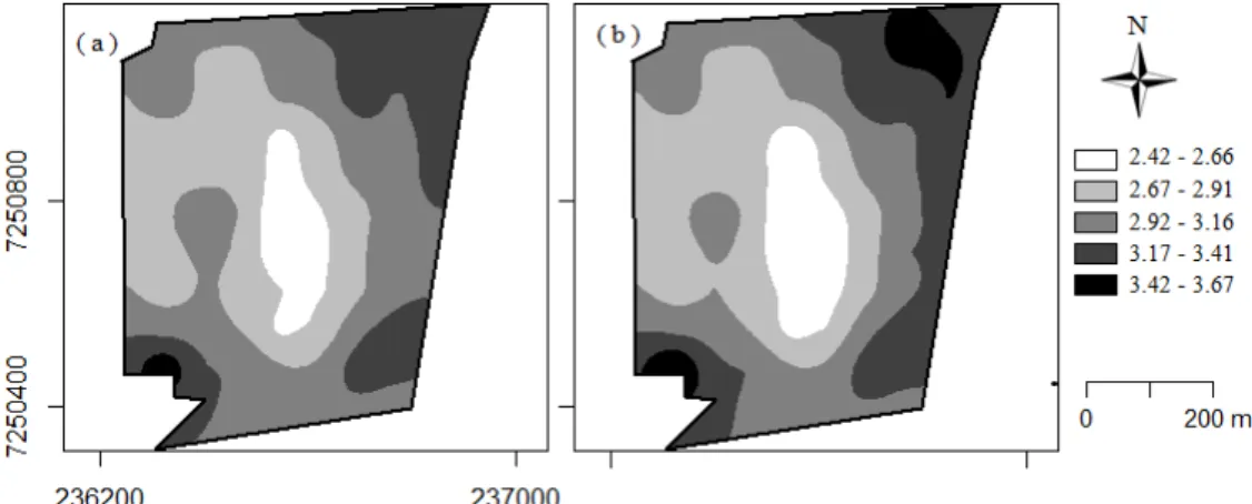
of the spatial linear regression model: ˆ₁ = 0.993, ˆ₂ = 0.021, ˆ₃ = 0.030, ˆ₁ = 0.248, ˆ₂ = 0.121, and ˆ₃ = 112.8, with a practical range of 328.0 m. Figure 4b shows the soybean yield map considering that the data have a normal distribution and shape parameter of the Matérn model

0.5



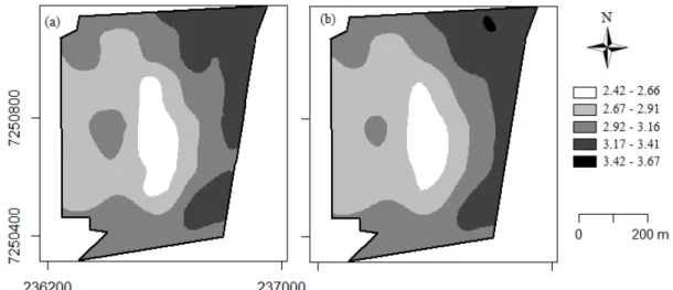
 with the following parameters estimated by the maximum likelihood of the spatial linear regression model: ˆ₁= 0.957, ˆ₂= 0.023, ˆ₃= 0.030, ˆ₁ = 0.298, ˆ₂ = 0.132, and ˆ₃ 133.4, with a practical range of 400.20 m.

An increase in area percentage was observed in the 1st, 2nd, and 5th classes of the map constructed with a normal distribution (Map 2) when compared to the map constructed with the reparameterized t-Student distribution (Map 1) (Figure 4 and Table 4). Consequently, the 3rd and 4th classes presented a reduction, with the 3rd class obtaining a greater reduction, equivalent to 6.08%, decreasing from 37.33 to 31.25% of the area.

FIGURE 4. (a) Map 1: soybean yield with reparameterized t-Student distribution with  0.050 and Matérn family model with shape parameter



0.5; (b) Map 2: soybean yield with normal distribution and Matérn family model with shape parameter



0.5.

TABLE 4. Area percentage at each map class of soybean yield constructed with the reparameterized t-Student distribution and normal distribution.

Class (t ha-1)

Map 1 % area

Map 2

% area Difference between maps (%)

2.42–2.66 8.07 10.33 2.26

2.67–2.91 30.68 30.80 0.12

2.92–3.16 37.33 31.25 6.08

3.17–3.41 23.25 23.20 0.05

3.42–3.67 0.67 4.31 3.64

Map 1 related to Figure 4a with the reparameterized t-Student distribution; Map 2 related to Figure 4b with the normal distribution.

For comparison between maps, the kappa accuracy index (K) was calculated. This index is considered an appropriate measure by Anderson et al. (2001) since it uses all elements of the error matrix constructed from omission errors and designation between maps (De Bastiani et al., 2012). The obtained value of K = 0.64 allows classifying it as a low similarity. Consequently, the maps constructed with reparameterized t-Student and normal distributions are dissimilar due to the influence of the discrepant point.

discrepant point in mapping is relevant.

FIGURE 5. (a) Map 1: soybean yield with reparameterized t-Student distribution with  0.050 and Matérn family model with shape parameter



0.5without point 6; (b) Map 2: soybean yield with normal distribution and Matérn family model with shape parameter



1.0 without point 6.

CONCLUSIONS

When applying the methodology proposed in this study for soybean yield data with the covariates average height and an average number of pods per plant, the parameters estimated by complete maximum likelihood using the reparameterized t-Student distribution presented differences in the estimates of parameters that define the spatial dependence structure when compared to those obtained from a normal distribution. Consequently, differences were observed in soybean yield maps obtained from the different methods. Thus, the use of reparameterized t-Student distribution is an alternative in studying data with discrepant values, showing the ability to decrease the influence of these points.

ACKNOWLEDGEMENTS

To the CNPq, CAPES, Araucária Foundation of the Paraná state and project FONDECYT 1150325 Chile, for the financial support to develop this research.

REFERENCES

Anderson J, Hardy E, Roach J, Witmer R (2001) A land use and land cover classification system for use with remote sensor data.. US Geological Survey Professional, Washington, DC, US Geological Survey Professional. 41p. (Technical Report Paper 964)

Assumpção RAB, Uribe-Opazo MA, Galea M (2011) Local influence for spatial analysis of soil physical

properties and soybean yield using student’s t-distribution. Revista Brasileira de Ciência do Solo 35(6):1917-1926. DOI: http://dx.doi.org/10.1590/S0100-06832011000600008

Assumpção RAB, Uribe-Opazo MA, Galea M (2014) Analysis of local influence in geostatistics using Students t-distribution. Journal of Applied Statistics 41(3):615-630. DOI:

http://dx.doi.org/10.1080/02664763.2014.909793

Bivand, R (2015) classInt: Choose Univariate Class Intervals. R package version 0.1-23. Available: https://cran.r-project.org/package=classInt.

De Bastiani F, Uribe-Opazo MA, Dalposso GH (2012) Comparison of maps of spatial variability of soil resistance to penetration constructed with and without covariables using a spatial linear model. Engenharia Agrícola 32(2):394-404. DOI:http://dx.doi.org/10.1590/S0100-69162012000200019

De Bastiani F, Cysneiros AHMA, Uribe-Opazo MA, Galea M (2015) Influence diagnostics in ellipitical spatial linear models. Test 24(2):322-340. DOI:http://dx.doi.org/10.1007/s11749-014-0409-z

Dempster A, Laird N, Rubin DB (1977) Maximum likehood estimation from incomplete data via the EM algorithm. Journal of the Royal Statistical Society 39(1):1-38.

EMBRAPA - Empresa Brasileira de Pesquisa Agropecuária (2011) Manual de métodos de análise de solo. Rio de Janeiro, Embrapa Solos, 2 ed. p212.

Galea M, Bonfarine H, Labra FV (2002) Influence diagnostics in structural erros-in-variables model under Student-t-distribution. Journal of Applied Statistics 29(8):1191-1204. DOI:

http://dx.doi.org/10.1080/0266476022000011265

Kano Y, Berkane M, Bentler P (1993) Statistical inference based on pseudo-maximum likelihood estimators in elliptical populations. Journal American Statistical Association 88(421):135-143. DOI: http://dx.doi.org/10.2307/2290706

Krippendorff K (2004) Content analysis: an introduction to its methodology. Beverly Hills, Sage Publications.

Lange KL, Little RJA, Taylor JMG (1989) Robust statistical modeling using the t distribution. Journal of the American Statistics 84(408):881-896. DOI:http://dx.doi.org/10.2307/2290063

Manghi RF, Paula GA, Cysneiros FJA (2016) On elliptical multilevel models. Journal of Applied Statistics 43(12):2150-2171. DOI:http://dx.doi.org/10.1080/02664763.2015.1134445

Matérn B (1986) Lecture notes in statistics. Springer, New York, p68-106.

Meyer D, Dimitriadou E, Hornik K, Weingessel A, Leisch F (2015) e1071: Misc Functions of the

Department of Statistics, Probability Theory Group (Formerly: E1071), TU Wien. R package version 1.6-7. Available: https://CRAN.R-project.org/package=e1071.

Michel PG, Kobiyama M (2015) Estimativa da profundidade do solo: parte 2- métodos matemáticos. Revista Brasileira de Geografia Física 8(4):1225-1243.

Nesi CN, Ribeiro A, Bonat WH, Ribeiro Jr PJ (2013) Verossimilhança na seleção de modelos para predição espacial. Revista Brasileira de Ciência do Solo 37(2):352-358.

DOI:http://dx.doi.org/10.1590/S0100-06832013000200006.

Novomestky F (2012) matrixcalc: Collection of functions for matrix calculations. R package version 1.0-3. Available: https://CRAN.R-project.org/package=matrixcalc.

Osorio F, Paula GA, Galea M (2007) Assessment of local influence in elliptical linear models with longitudinal structure. Computacional Statistics & Data Analysis Journal 51(9):4354-4368.

R Core Team. (2016) A language and environment for statistical computing. Vienna, Foundation for Statistical Computing.

Ribeiro Junior PJ, Diggle PJ (2016) geoR: Analysis of Geostatistical Data. R package version 1.7-5.1. Available: https://CRAN.R-project.org/package=geoR.

Uribe-Opazo MA, Borssoi JA, Galea M (2012) Influence Diagnostics in Gaussian Spatial Linear Models. Journal of Applied Statistics 39(3):615-630. DOI:http://dx.doi.org/10.1080/02664763.2011.607802 Vieira SR (2000) Geoestatística em estudos de variabilidade espacial do solo. Tópicos em Ciências do Solo. Revista Brasileira de Ciência do Solo 1:1-54.