AN ANALYSIS OF THE TIMES OF STOPPAGES OF EQUIPMENTS IN A FOOD INDUSTRY: A CASE STUDY
UMA ANÁLISE DOS TEMPOS DE PARADAS DE EQUIPAMENTOS EM UMA INDÚSTRIA DE ALIMENTOS: UM ESTUDO DE CASO
Marcos Alberto Claudio Pandolfi* E-mail: marcoscps2011@yahoo.com.br Denis Komninakis** E-mail: denis.komninakis@gmail.com
Cláudio Luis Piratelli* E-mail: clpiratelli@uniara.com.br
Vera Mariza Henriques de Miranda Costa** E-mail: verammcosta@uol.com.br Jorge Alberto Achcar** E-mail: achcar@fmrp.usp.br
*Faculdade de Tecnologia de Taquaritinga (FATEC), Taquaritinga, SP, Brazil.
**Universidade de Araraquara(UNIARA), Araraquara, SP, Brazil
Abstract: The main objective of this study is to analyze the data related to the times of stoppages of equipment due to several causes in a food industry in the fruit sector located in São Paulo State, Brazil. Several causes can affect the performance of such equipment as the industry sector where the equipment is used, the type of equipment, the period of operation and the harvest (year).The results of this analysis could be of great interest to managers of industry in terms of better planning on the use of machinery, detection of the risk factors for the use of machinery and minimization of maintenance shutdowns.
Keywords: Times of stoppages. Statistical modeling. Analysis of variance. Regression models.
Resumo: O principal objetivo deste estudo é analisar os dados relacionados aos tempos de paradas de equipamentos, por diversas causas, em uma indústria de alimentos no setor de frutas, localizada no estado de São Paulo, Brasil. Diversas causas podem afetar o desempenho de tais equipamentos, como o setor da indústria onde o equipamento é utilizado, o tipo de equipamento, o período de operação e a colheita (ano). Os resultados dessa análise podem ser de grande interesse para os gestores da indústria no setor, em termos de melhor planejamento sobre o uso de máquinas, detecção dos fatores de risco para o uso dessas máquinas e minimização de paradas para manutenção.
Palavras-chave: Tempos de parada. Modelagem estatística. Análise de variância. Modelos de regressão.
1 INTRODUCTION
The study of variations in the times of stoppages of equipment used in an industry are of great interest to the industrial engineers. The statistical modeling of these data is useful for diagnosis (performance indicators by means of the queuing theory), inference
or simulation, especially for decision making on investment, planning production, allocation of maintenance, among many others. The discovery of possible factors that act in these variations can be of great interest to engineers and industrial managers.
The main purpose of this study is to analyze a dataset related to the times of stoppages due to equipment failures in an industry of the food sector in São Paulo State, Brazil. For this analysis, initially it will be used an variance model considering data transformed to a logarithmic scale to verify possible differences in average times due to several categorical factors. In a second analysis of the data, it will be used a multiple linear regression model considering the transformed data to confirm which factors are most important in the variability of the times of stoppages and also to be used in forecasts. A third analysis will be considered using reliability modeling techniques assuming the data in the original scale.
The study of the reliability of components and systems and possible causes that can lead to large losses is of great interest for the industries to minimize costs. The analysis of data related to the times up to failures of different equipment for food industry can lead to better strategies for maintenance for the different types of equipment and possible discoveries of factors that lead to better performance of equipment, such as sector, season, type of equipment, models of equipment, work periods, temperature, among many other factors.
The study of maintenance and reliability of equipment has been extensively studied in the literature to optimize the industrial performance and minimize losses (ALMEIDA, 2007; KARDEC; NASCIF, 2001; DHILLON, 1999; MOUBRAY, 1997; ZHANG; JARDINE, 1998; CHRISTER et al., 1998; NAKAGAWA, 2005; BILLINTON; ALLAN, 1983; BLANCHARD; FABRYCKY, 1998; KELLY, 1984; VIVEROS et al. 2013; DÍAZ CONCEPCIÓN; CASTILLO SERPA; VILLAR LEDO, 2017).
Studies on the times up to failures and discoveries of factors that can increase these times are important for the industrial managers to make decisions that can mean significant gains for the industry (BRWON; KAHR; PETERSON, 1974; AL-NAJJAR, 1996).
Monitoring indicators are essential to measure and to verify the actual performance of the maintenance system. These indicators of reliability usually presented in the literature are: mean time to failure (MTTF) or mean time between failures (MTBF), mean time to repair (MTTR), and availability (A) (MENDES; RIBEIRO, 2015; ZADHOOSH; FATAHI, 2015). The MTTR, in this study denoted as stoppage times, includes required time for repairing failures troubleshooting, resolution downtime, repairs, and any tests that we need to ensure the elimination of the problem (TSAROUHAS; ARVANITOYANNIS; AMPATZIS, 2009).
The identification of appropriated probability distributions for the stoppage times is of great importance for better studies and consequently better inferences and predictions in industrial applications (MONTGOMERY; RUNGER, 2010).
There are two approaches to identify the distributions for the failure–repair data: 1) the empirical method, that derives the empirical distributions directly from the failure data, and does not require the estimation of the distribution’s parameters; 2) theoretical distributions method, that focuses on identifying the candidate theoretical distribution, estimating the parameters and performing a goodness-of-fit test (TSAROUHAS; ARVANITOYANNIS; AMPATZIS, 2009).
In this way, a popular statistical lifetime model given by the Weibull distribution (a theoretical method) has been much used in the analysis of medical lifetime data (ACHCAR; BROOKMEYER; HUNTER, 1985) or for industrial lifetimes (BABUY; JAYABALAN, 2009; NELSON, 2004; MEEKER; ESCOBAR, 1998) given its great flexibility of fit. Reliability studies are related to the quality and industrial productivity, and have been the goal of many researchers and industrial engineers, since the competitiveness of an industry is associated with better reliability (NELSON, 2004; BILLINTON; ALLAN, 1983).
Based on the literature (TURRIONI; MELLO, 2012; CAUCHICK MIGUEL, 2010; YIN, 2005; BERTRAND; FRANSOO, 2002), methodologically this work could be classified as applied, objective and of descriptive quantitative approach. Bertrand and Fransoo (2002) define the quantitative research in production engineering such as the
one where it is possible to model a problem that presents variables whose relationships are causal and quantitative.
In this sense, it becomes possible to quantify the behavior of the dependent variables in a specific field, enabling the researcher to make predictions. In general, the quantitative research uses mathematical modeling, statistical or computational (simulation) methods. In this paper, as research techniques, it will be used a bibliographic research and intensive direct observation, according to the classification of Lakatos and Marconi (2008) or the bibliographic research and case study, according to the classification of Gil (2008) and Yin (2005).
The article is organized as follows: in section 2, it is introduced the problem and a descriptive analysis of the data; In the section 3 it is introduced a statistical modeling for the stoppage times; In section 4 it is introduced a statistical analysis for the times of stoppages considering different statistical models; In section 5 it is introduced a discussion of the obtained results and some final considerations.
2 PRESENTATION OF THE PROBLEM AND DESCRIPTIVE ANALYSIS OF THE DATA
The studied food industry is located in the São Paulo State, southeast of Brazil and operates in the processing of tropical fruit for manufacture of concentrated juices. The main raw materials of the company are: mango, guava, pineapple, passion fruit and acerola, being the product obtained classified as a semi-industrialized, once the processed product will serve as the raw material for manufacturers of ready-to-drink juices, jams, jellies and others.
Strategically located with facilitating logistics for agricultural supplies, proximity of various suppliers, labor availability and flow of production, and designed for internal market or export, the plant that served as the basis for the study has an estimated processing capacity of 500 tons of fruit per day, available in a period of months ranging from October to March each year. The company has a staff of approximately 200 employees where 150 are directly linked to the production process.
One of the characteristics of the processing fruit industries is the seasonality in the supply of raw material, leading to a carefully planning of industrial operations to seek strategies to optimize the maximum use of the needed resources: labor, raw materials, machinery, some other inputs and time.
In the constant search for competitiveness, companies seek to eliminate waste, increasing productivity, with fewer resources, more quickly, and therefore at a lower cost. For this reason, efficiency indicators of industrial processes have been implemented to facilitate the identification of weak points in the production line and thus enabling the deployment of operational strategies and management to ensure the highest possible productivity.
Another remarkable characteristic of the processing fruit industry is that the production process is classified as a continuous process having a physical arrangement for each different product, which leads to a system with a high production volume and a low variety of products.
Therefore, it is essential to have a high performance in the availability of equipment with minimization due to the loss of time due to failures in machines since consequently maintenance interventions usually represent a waste that can not be recovered besides costs not foreseen in advance.
A macro overview of business processes can be seen in Figure 1, which represents the simplified flow chart of the fruit processing.
The equipment is positioned according to the sequence of operations and the related processes are interdependent to each other with low level of inventory in the process. In general, the automated process works without interruption. The new technology has substantially changing the productive processes manufacturing, both in order to allow more automation, with evident impact on productivity and consistency and reliability of the production, as in the challenge of traditional trade-off between efficiency and flexibility of the processes. In large-scale production, productive systems are organized in order to more easily standardize the productive resources (machines, men and materials) with new working methods and controls, contributing to a greater efficiency of the system, with a consequent reduction of costs.
The measurement of the stoppages and loss of time was monitored in the last step of the industrial process, the bottling stage, considered as the bottleneck of the production line.
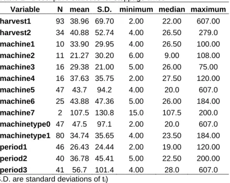
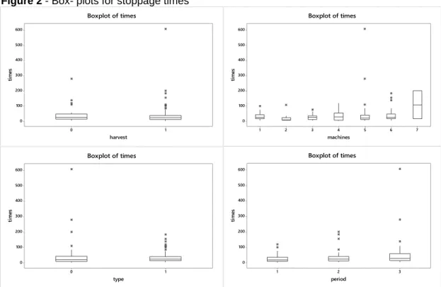
The company works with three production periods. The times of downtime due to equipment failures are classified into seven types: machines M1 (discharge of fruit), M2 (grinding), M3 (depulping), M4 (concentration), M5 (bottling), M6 (waste) and M7 (utilities).The times of downtime may be affected by some factors such as type of equipment (E for electrical machine, M for mechanical machine) and work period (1 (first), 2 (second), 3 (third)).The descriptive statistics of these data are presented in Table 1. Figure 2 shows the box-plots graphs of the mean time between daily arrivals obtained using the MINITAB® software version 14.
From the results in Table 1 and Figure 3, it is possible to infer that there is a great variability in the stoppage times due to failures and the industry has great interest in identifying the factors that affect this variability. This is also confirmed by the box-plots graphs in Figure 2, where we can observe that the distribution for the times of stoppage in the original scale has an asymmetrical form.
The application of descriptive statistics to the failure data is very effective for drawing conclusions with regard to the identification of most important failures (TSAROUHAS; ARVANITOYANNIS; AMPATZIS, 2009).
By these results, it is observed that the machines (equipment) and machine types have different average times due to breakage; this fact apparently also occurs for periods (the period 1 apparently has smaller times of equipment stoppages).
In Figure 3, it is presented the histograms for all stoppage times in the original scale and in the transformed scale (logarithmic scale). We observe better symmetry for the transformed data (an indication of approximate normality).
In Figure 4, it is presented the normal probability plot for the transformed data (logarithmic scale); from this graph we observe approximate normality for the transformed data (approximately linear relationship). In Figure 5, the box-plots of logarithms of the stoppage times are presented.
Table 1 - Descriptive statistics for stoppage times
Variable N mean S.D. minimum median maximum harvest1 93 38.96 69.70 2.00 22.00 607.00 harvest2 34 40.88 52.74 4.00 26.50 279.0 machine1 10 33.90 29.95 4.00 26.50 100.00 machine2 11 21.27 30.20 6.00 9.00 108.00 machine3 16 29.38 21.00 5.00 26.00 75.00 machine4 16 37.63 35.75 2.00 27.50 120.00 machine5 47 43.7 94.2 4.00 20.0 607.0 machine6 25 43.88 47.36 5.00 26.00 184.00 machine7 2 107.5 130.8 15.0 107.5 200.0 machinetype0 47 47.5 97.1 2.00 20.0 607.0 machinetype1 80 34.74 35.65 4.00 23.50 184.00 period1 46 26.43 24.44 2.00 19.00 120.00 period2 40 36.78 45.41 5.00 22.50 200.00 period3 41 56.7 101.4 4.00 28.0 607.0 (S.D. are standard deviations of ti)
Figure 2 - Box- plots for stoppage times 1 0 600 500 400 300 200 100 0 harvest tim es Boxplot of times 7 6 5 4 3 2 1 600 500 400 300 200 100 0 machines tim es Boxplot of times 1 0 600 500 400 300 200 100 0 type tim es Boxplot of times 3 2 1 600 500 400 300 200 100 0 period tim es Boxplot of times
Figure 3 - Histograms for the stoppage times in original and logarithm scales
600 500 400 300 200 100 0 -100 70 60 50 40 30 20 10 0 Mean 39,47 StDev 65,39 N 127 times Fr eq ue nc y Histogram of times 6 5 4 3 2 1 35 30 25 20 15 10 5 0 Mean 3,111 StDev 1,003 N 127 log(times) Fr eq ue nc y Histogram of log(times)
To optimize the operation of the production line, the aim is to proceed in improvements. The best way is to begin with the failures that have the most important negative impact on the smooth operation of the line (TSAROUHAS; ARVANITOYANNIS; AMPATZIS, 2009).
To find out which factors are significant in the stoppage times, we assume different statistical analyses for the stoppage data assuming different statistical models.
Figure 5 - Box- plots for logarithms of stoppage times
1 0 7 6 5 4 3 2 1 0 harvest lo g( tim es ) Boxplot of log(times) 7 6 5 4 3 2 1 7 6 5 4 3 2 1 0 machines lo g( tim es ) Boxplot of log(times) 1 0 7 6 5 4 3 2 1 0 type lo g( tim es ) Boxplot of log(times) 3 2 1 7 6 5 4 3 2 1 0 period lo g( tim es ) Boxplot of log(times)
3 STATISTICAL MODELING FOR THE STOPPAGE TIMES
For a first statistical analysis of the stoppage times of the food industry assuming the data transformed to a logarithm scale, we use ANOVA (analysis of variance) methods to compare means of the different groups. Analysis of variance (ANOVA) is in a simplified way a collection of statistical models in which the observed variance in a response variable is partitioned into components attributable to different sources of variation. In this way, ANOVA provides a statistical test of whether or not the means of
several groups are all equal, that is, a generalization of t-tests to more than two groups. Different approaches are presented in the literature for analysis of variance; the most common uses a linear model that relates the response to the treatments and blocks (BOX; HUNTER; HUNTER, 1978; MONTGOMERY, 2010). Using ANOVA with only one classification, the null hypothesis establishes that all groups are simply random samples of the same population. Rejection of the null hypothesis implies that different treatments or groups have different means. The normal-linear model based ANOVA analysis assumes independence, normality and homogeneity of the variances of the residuals.
As a second statistical analysis also considering the logarithms of the stoppage times, we use multiple linear regression models analysis. Regression analysis is used for prediction and forecasting in many scientific areas (DRAPER; SMITH, 1998; FOX, 1997; RAWLINGS; PANTULA; DICKEY, 1998). This approach provides concepts and methods for modeling and analyzing several variables by relating a dependent variable Yi ,i=1,…,n where n is the sample size with one or k fixed independent variables given in
a vector denoted as xi = (x1i,….,xki). Indeed, in the regression models there is
associated to the vector of independent variables, a vector of unknown regression parameters, denoted as β.
A general regression model is defined as,
Yi = f(xi, β) + εi (1)
where f(xi, β) is a specified function and the error term εi is a random variable assumed
to have a specified probability distribution. This random error includes all other factors which could influence the dependent variable Y not included in the regression model.
A particular regression model is a linear model, which is given by
Yi = β0 + β1 x1i +….+ βk x1i + εi (2)
for i=1,…,n where the vector of regression parameters is given by β = (β0 , β1 , ….βk)
and the error term εi is a random variable assumed to be normally distributed with mean
As a third statistical analysis, we use lifetime models considering the stoppage times in the original scale. Lifetime analysis is related to the statistical modeling dealing with failures of components or mechanical systems, where the random variable of interest is defined for continuous positive values. This methodology is also called reliability analysis in engineering applications. Different probability distributions could be used to analyze the lifetimes. One of the most popular models used to analyze lifetimes is the Weibull distribution (WEIBULL, 1951). Among the great advantages of the Weibull distribution we can point out its versatility and easiness of use. The distribution provides a good fit for a wide range/variety of data sets (LAWLESS, 1982). Other lifetime distributions commonly used to analyze lifetime data are: the exponential distribution that is a special case of the Weibull distribution, the log-normal distribution, the gamma distribution or the generalized gamma distribution (LAWLESS, 1982; MEEKER; ESCOBAR, 1998). We also can have the presence of some covariates affecting the lifetimes. In this direction, we could assume a Weibull parametric regression model affecting one or more parameters of the Weibull distribution.
The Weibull distribution with two parameters (WEIBULL, 1951; JOHNSON; KOTZ; BALAKRISHNAN, 1994; NELSON, 2004; COLOSIMO; GIOLO, 2006), has probability density function given by,
f(ti) = exp{ - ( )α} (3)
where ti>0 denotes the stoppage times of the machines. The parameters λ and denote
respectively, the scale and shape parameters. Different values of give different shapes for the distribution, that is, we have a great flexibility of fit for the times between stoppages.
The reliability function for time t* is given by,
Note that (4) represents the probability that the stopping times are greater than a fixed value t* (t*≥0).
Assuming a Weibull distribution with probability density function (3), we have,
R(t*) = exp{ - ( )α} (5)
The hazard function h(t) (or instantaneously failure rate) of the Weibull distribution (NELSON, 2004; MEEKER; ESCOBAR, 1998) is given from the relation h(t) = f(t)/R(t) by,
h(t) = αtα-1/λα 6)
Observe that if α=1, we have an exponential distribution, that is, the exponential distribution is a special case of the Weibull distribution. The hazard function h(t) given by (6) is strictly increasing for α> 1 (that is, the times of occurrence of events of interest are smaller in the terminology of industrial reliability), strictly decreasing for α< 1 (that is, the times of occurrence of events of interest are larger or last longer in the terminology of industrial reliability), and constant for α = 1. Thus, there is a great flexibility of fit for the data.
In presence of a vector of covariates denoted as xi= (x1i,….,xki), we assume a
Weibull regression model for the stoppage times defined by,
log(ti) = β0 + β1 x1i +….+βk x1i + σ*εi (7)
where ti are the stoppage times; β0, β1, …. βk are the regression parameters. The
parameter σ* is related to the shape parameter of the Weibull distribution (3) by the relationship σ* = 1/ α. The term εi in (7) is a random quantity with an extreme value
distribution (NELSON, 2004; LAWLESS, 1982)
also defined as an extreme value distribution of type I (minimum) or Gumbel distribution (GUMBEL, 1954)with a probability density function given by f(ε) = exp{ ε – exp(ε)}, - < ε < .
Also note that from model (7), the scale parameter λ defined in (3) is related with the covariates vector from the relationship,
λi = exp(β0 + β1 x1i +….+ βk x1i) (8)
that is, the regression model defined by (7) defines a regression model in the scale parameter (LAWLESS, 1982) assuming the same shape parameter.
4 STATISTICAL ANALYSIS FOR THE STOPPAGE TIMES
Initially we consider an analysis of variance model with a classification considering the qualitative variables machines, types of machines, harvest and periods for the transformed data (logarithm of stoppages) using the MINITAB® software.
In Table 2 we have those results.
Table 2 - Analysis of variance for the logarithms for stoppage times Source DF SS MS F p-value Harvest 1 0.57 0.57 0.57 0.453 Error 125 126.23 1.01 Total 126 126.8 Source DF SS MS F p-value Machine 6 6.98 1.163 1.17 0.33 Error 120 119.825 0.999 Total 126 126.805 Source DF SS MS F p-value Machinetype 1 0.2 0.2 0.2 0.654 Error 125 126.6 1.01 Total 126 126.8 Source DF SS MS F p-value Period 2 4.784 2.392 2.43 0.092 Error 124 122.021 0.984 Total 126 126.805
(D.F. are degrees of freedom; SS are sums of squares; MS are mean squares; F is the reference value for the Snedecor F-distribution).
Source: Authors
From the results of Table 2, it is observed that the period factor leads to some significant difference between the stoppage times (logarithmic scale) since the p-value is
equal to 0.092 (significance with a 10% significance level) .The other factors do not show significant differences between the levels of each factor.
As a second statistical data analysis, we consider a multiple linear regression model assuming independent errors with normal distribution N(0,𝜎2) with constant
variance 𝜎2.
The response variables are given by the logarithms of the stoppage times and the explanatory variables are given by: a “dummy” or categorical variable for the mechanical type of machine =1, 0= other part; a “dummy” or categorical variable for the harvest 1=1, 0=other part; a “dummy” or categorical variable for the machine M1=1, 0=other part; a “dummy” or categorical variable for the machine M2=1, 0=other part; a “dummy” or categorical variable for the machine M3=1, 0=other part; a “dummy” or categorical variable for the machine M4=1, 0=other part; a “dummy” or categorical variable for the machine M5=1, 0=other part; a “dummy” or categorical variable for the machine M6=1, 0=other part; a “dummy” or categorical variable for the period 1=1, 0=other part; a “dummy” or categorical variable for the period 2=1, 0=other part and the following multiple linear regression model (see (2)) fitted by the least squares estimation method (use of the software Minitab):
log(stoppage time) = 4.48 – 0.249(indicator harvest1) - 0.831(indicator machine M1) – 1.57(indicator machine M2) - 1.01(indicator machine M3) – 1.05(indicator machine M4) - 1.08(indicator machine M5) – 0.776 (indicator machine M6) - 0.497 (indicator period 1) – 0.207 (indicator period 2) + 0.118(mechanical machine) (9)
Table 3 - LSE for the regression coefficients assuming the multiple linear regression model for the stoppage time logarithms
predictor LSE SE T P-value
Constant 4.4795 0.7341 6.1 0 indicator harvest=1 -0.2491 0.2254 -1.11 0.271 indicator machine M1=1 -0.8309 0.8101 -1.03 0.307 indicator machine M2=1 -1.5687 0.8091 -1.94 0.055 indicator machine M3=1 -1.0108 0.7676 -1.32 0.19 indicator machine M4=1 -1.0545 0.7758 -1.36 0.177 indicator machine M5=1 -1.0846 0.7205 -1.51 0.135 indicator machine M6=1 -0.7763 0.7837 -0.99 0.324 indicator Period=1 -0.4969 0.2178 -2.28 0.024 indicator Period =2 -0.2067 0.2266 -0.91 0.364 indicator Mechanical machine type 0.1179 0.2492 0.47 0.637
(LSE are the least squares estimators; SE are the standard-errors of the estimators; T is the reference value of the Student-t distribution).
Source: Authors
In Table 3, we have the obtained estimates, the standard-errors of the least squares estimates (LSE), the obtained values for the t-Student distribution test and the p-values associated with each regression parameter.
From the results of Table 3, it is observed that the period factor leads to a significant difference between the stoppage times (logarithmic scale) since the p-value associated with the period 1 when compared with other periods is equal to 0.024 (significance with a 5% significance level equals), that is, the period 1 has smaller machines stoppage times since the regression coefficient associated with the variable "dummy" indicator of period 1 has negative signal. In the same way it is possible to detect some significance of the machine M2 since the observed p-value is equal to 0.055 (significance with a significance level close to 5%).
In Figure 6, we have the graphs of the residuals of the fitted regression model. It is observed that the assumptions for the validity of the inferences are verified (normality of the errors and constant variance).
Figure 6 - Plots of the residuals (multiple regression model)
As a third analysis, we assume a Weibull regression model (see (7)) for the stoppage times defined by,
log(ti) = β0 + β1 indicator harvest1i + β2 indicator machine M1i + β3 indicator machine M2i +
β4 indicator machine M3i + β5 indicator machine M4i + β6 indicator machine M5i +
β7 indicator machine M6i + β8 indicator period1i + β9 indicator period2i + β10 indicator
machine typei + σ*εi (10)
Where ti are the stoppage times and have an extreme value distribution (see (7)).
Also, note that the scale parameter λ defined in (3) are related with the covariates from the relationship,
λi = exp{ β0 + β1 indicator harvest1i + β2 indicator machine M1i + β3 indicator machine M2i +
β4 indicator machine M3i + β5 indicator machine M4i + β6 indicator machine M5i +
β7 indicator machine M6i + β8 indicator period1i + β9 indicator period2i + β10 indicator
machine typei } (11)
That is, the regression model defined by (10) defines a regression model in the scale parameter (LAWLESS, 1982), assuming the same shape parameter.
For the regression model (10), we estimate the regression parameters β0 , β1 , β2
, β3 , β4 , β5 , β6 , β7 , β8 , β9 , β10 and the parameter σ* using maximum likelihood
methods (MOOD; GRAYBILL; BOES, 1974). The maximum likelihood estimators for β0 ,
β1 , β2 , β3 , β4 , β5 , β6 , β7 , β8 , β9 , β10 and σ* are obtained by maximizing the
likelihood function
L(λ,α) = ) where f(εi ) = exp{ εi – exp(εi)}, i = 1,2,..,n and σ*εi = log(ti) -
[β0 + β1 indicator harvest1i + β2 indicator machine M1i + β3 indicator machine M2i + β4
indicator machine M3i + β5 indicator machine M4i + β6 indicator machine M5i +
β7 indicator machine M6i + β8 indicator period1i + β9 indicator period2i + β10 indicator
machine typei ]
In practice, in general, we maximize the logarithm of the likelihood function in the determination of the maximum likelihood estimators (MLE).
For the data analysis of the stoppage times, we assume the Weibull distribution with density (3) and the regression model (10). From the software MINITAB version 14, we obtained the maximum likelihood estimators (see Table 4).
Table 4 - MLE for the parameters of the Weibull regression model
Preditor MLE SE Z p-value 95% Confidence Interval lower upper intercept 539.032 0.748632 7.20 0.000 392.303 685.761 mechanicalmachine -0.316216 0.253245 -1.25 0.212 -0.812567 0.180135 harvest1 -0.102030 0.220270 -0.46 0.643 -0.533751 0.329690 machine M1 -0.870514 0.810378 -1.07 0.283 -245.882 0.717798 machine M2 -151.327 0.798775 -1.89 0.058 -307.884 0.052303 machine M3 -134.496 0.753896 -1.78 0.074 -282.257 0.132648 machine M4 -0.882387 0.775862 -1.14 0.255 -240.305 0.638275 machine M5 -114.163 0.721043 -1.58 0.113 -255.485 0.271590 machine M6 -0.717971 0.759869 -0.94 0.345 -220.729 0.771345 period 1 -0.794484 0.218147 -3.64 0.000 -122.204 -0.366924 period 2 -0.588971 0.232824 -2.53 0.011 -104.530 -0.132643 shape(a) 103.431 0.0667837 0.911364 117.385
From the results of Table 4, we also observe that the period factor leads to a significant difference between the stoppage times since the p-value associated with the period 1 when compared to the other periods is lower than 0.001 (significance with a 5% significance level) and the period 2 also indicates a significant difference (p-value equals to 0.011), that is, the periods 1 and 2 have smaller stoppage times of the machines.
In the same way it is possible to detect some significant difference between machines M2 and M3 since the observed p-values are respectively equal to 0.058 and 0.074 (significance at a 10% significance level).
Observe that the confidence interval for the shape parameter α includes the value 1, an indication that the exponential distribution also could be fitted to the data. From the results of Table 4, we see that the use of the Weibull distribution to analyze the data set (times until failure) in the original scale leads to greater sensitivity in the detection of significant effects than using a linear regression model for the transformed data (logarithm scale) with normal errors (that is, assuming a log-normal distribution for the original data).
5 DISCUSSION OF THE RESULTS OBTAINED AND CONCLUSIONS
The presented statistical analysis for the data from the Brazilian industry of the food sector can be of great interest in identifying the causes of the great variability in the stoppage times of different equipment used in the production line. Often these equipments are of great cost and the identification of possible factors that lead to the increase of these stoppage times, that is, less stopping occurrences in a fixed time period, can be of great industrial interest.
The use of different statistical modeling can lead to major gains in inferences and possible forecasts. This was observed in the case study using techniques of ANOVA (analysis of variance) and multiple regression models to the data transformed to a logarithm scale assuming normal errors with constant variance and Weibull regression models assuming the stoppage times in the original scale.
Using these different statistical models, it was possible to detect two main factors that affect the variability of the data: periods of the industry and machinery. In a future
study, it would also be possible to incorporate this in these models other factors such as seasons of the year, temperature, relative humidity of the air between several other factors.
It is important to emphasize that the statistical approach taken in this article can bring benefits for the various production systems.
REFERENCES
ACHCAR, J. A.; BROOKMEYER, R. S.; HUNTER, W. G. An application of Bayesian analysis to medical follow-up data. Statistics in Medicine, v.4, p.509-520, 1985.
https://doi.org/10.1002/sim.4780040411
ALMEIDA, M. T. Manutenção preditiva: confiabilidade e qualidade. Itajubá: Escola Federal de
Engenharia, 2007. Available in: www.mtaev.com.br/download/mnt1.pdf.
AL-NAJJAR, B. Total quality maintenance. An approach for continuous reduction in costs of quality products, J. of Quality in Maintenance Engineering, v. 2, n. 3, p. 4-20, 1996.
https://doi.org/10.1108/13552519610130413
BABUY, A. S.; JAYABALAN, V. WEIBULL Probability Model for Fracture Strength of Aluminium (1101) - Alumina Particle Reinforced Metal Matrix Composite. Journal of Material Science
Technology, v. 25, n. 3, p. 341-343, 2009.
BERTRAND, J. W. M.; FRANSOO, J. C. Operations management research methodologies using quantitative modeling. Journal of Operations & Production Management, v.22, 2, p.241-261,
2002.https://doi.org/10.1108/01443570210414338
BILLINTON, R.; ALLAN, R. N. Reliability evaluation of engineering systems: concepts and
techniques. Boston, Pitman Books Limited, 1983. https://doi.org/10.1007/978-1-4615-7728-7
BLANCHARD, B. S.; FABRYCKY, W. J. Systems engineering and analysis. 3rd ed. Upper Saddle River, NJ: Prentice-Hall, 1998.
BOX, G. E. P.; HUNTER, W. G.; HUNTER, J. S. Statistics for experimenters. New York: John Wiley & Sons, 1978.
BRWON, R.V.; KAHR, A.S.; PETERSON, C. Decision analysis for the manager. New York : Reinhardt & Winston, 1974.
CAUCHICK MIGUEL, P. A. Adoção do estudo de caso na engenharia de produção. In: CAUCHICK MIGUEL, P. A. (Org.) Metodologia de pesquisa em engenharia de produção e
gestão de operações. Rio de Janeiro: Elsevier, 2010, p. 129-143.
CHRISTER, A. H.; WANG, W.; SHARP, J.; BAKER, R. D. A case study of modelling preventative maintenance of a production plant using subjective data. Journal of the
COLOSIMO, E.; GIOLO, S. R. Análise de sobrevivência aplicada. Edgard Blucher, 2006. DHILLON, B. S. Engineering maintainability. Houston: Gulf Publishing Company, 1999.
https://doi.org/10.1016/B978-088415257-6/50004-1
DÍAZ CONCEPCIÓN, A.; CASTILLO SERPA, A. D.; VILLAR LEDO, L. Instrumento para evaluar el estado de la gestión de mantenimiento en plantas de bioproductos: un caso de estudio.
Ingeniare. Revista chilena de ingeniería, v.25, n.2, p.306-313, Jun.
2017.https://doi.org/10.4067/S0718-33052017000200306
DRAPER, N. R.; SMITH, H. Applied Regression Analysis, Wiley Series in Probability and
Statistics, 1998. https://doi.org/10.1002/9781118625590
FOX, J. Applied regression analysis: linear models and related methods. SAGE, 1997. GIL, A. C. Como elaborar projetos de pesquisa. 4. ed. São Paulo: Atlas, 2008.
GUMBEL, E. J. Statistical theory of extreme values and some practical applications, Applied
Mathematics, series 33, U.S. Department of Commerce: National Bureau of Standards, 1954. https://doi.org/10.4067/S0718-33052013000100011
JOHNSON, N. L.; KOTZ, S.; BALAKRISHNAN, N. Continuous univariate distributions, v. 1,
Wiley series in probability and mathematical statistics: applied probability and statistics (2nd Ed).
Wiley& Sons, 1994.
KARDEC, A.; NASCIF, J. Manutenção: função estratégica. 2ed. Rio de Janeiro: Qualitymark Ed., 2001.
KELLY, A. Maintenance planning and control: London: Butterworths, 1984.
LAKATOS, E. M.; MARCONI, M. A. Fundamentos de metodologia científica. 6. ed. São Paulo: Atlas, 2008.
LAWLESS, J. F. Statistical models and methods for lifetime data, Wiley series in probability and mathematical statistics, Wiley & Sons, 1982.
MEEKER, W. Q.; ESCOBAR, L. A. Statistical methods for reliability data, Wiley & Sons. 1998.
MENDES, A. A.; RIBEIRO, J.L.D. Study of the quantitative methods that support RCM operation. IEEE Conference: Reliability and Maintainability Symposium., 2015.
https://doi.org/10.1109/RAMS.2015.7105162
MONTGOMERY, D. C.; RUNGER, G. C. Applied statistics and probability for engineers, 5nd
Edition. Wiley & Sons, 2010.
MOOD, A. M.; GRAYBILL, F. A.; BOES, D. C. Introduction to the theory of statistics. Publisher: McGraw-Hill 1974.
MOUBRAY, J. Reliability-centered maintenance. New York, NY: Industrial Press, 1997. NAKAGAWA, T. Maintenance theory of reliability. London: Springer, p. 201-229, 2005. NELSON, W. Applied life data analysis. Wiley – Blackwell, 2004.
RAWLINGS, J. O.; PANTULA, S. G.; DICKEY, D. A. Applied Regression Analysis: a research
tool, second edition, Springer Verlag, 1998. https://doi.org/10.1007/b98890
TSAROUHAS, P. H.; ARVANITOYANNIS, I. S.; AMPATZIS, Z. D. A case study of investigating reliability and maintainability in a Greek juice bottling medium size enterprise (MSE). Journal of
Food Engineering, v. 95, n.3, p.479-488, 2009. https://doi.org/10.1016/j.jfoodeng.2009.06.011
TURRIONI, J. B.; MELLO, C. H. P. Metodologia de pesquisa em engenharia de produção: estratégias, métodos e técnicas para condução de pesquisas quantitativas e qualitativas. Itajubá: UNIFEI, 2012.
VIVEROS, P.; STEGMAIER, R.; KRISTJANPOLLER, F.; BARBERA, L.; CRESPO, A. Propuesta de un modelo de gestión de mantenimiento y sus principales herramientas de apoyo. Ingeniare.
Revista chilena de ingeniería, v. 21, n. 1, p. 125-138, Enero/Abril 2013.
WEIBULL, W. A statistical distribution function of wide applicability, Journal of Applied
Mechanics – ASMC, v. 18, n. 3, p. 293 – 297, 1951.
YIN, R. K. Estudo de caso: planejamento e métodos. Trad. D. Grassi. 3 ed. Porto Alegre: Bookman, 2005.
ZADHOOSH, M.; FATAHI, A. A. Simultaneous effect of RCM key indicators, related to
equipment lifecycle for maintenance strategies (in production systems). International Journal
of Engineering & Technology, v.4, n.3, p.439-445, 2015. https://doi.org/10.14419/ijet.v4i3.4006
ZHANG, F.; JARDINE, A.K.S. Optimal maintenance models with minimal repair, periodic overhaul and complete renewal, IIE Transactions, 30, 1109-1119, 1998.
https://doi.org/10.1080/07408179808966567
Artigo recebido em: 08/01/2019 e aceito para publicação em: 03/03/2020 DOI: http://dx.doi.org/10.14488/1676-1901.v20i1.3525