GBT-Based Buckling Analysis using the Exact Element Method

Proceedings of the 7th International Conference on Coupled Instabilities in Metal Structures Baltimore, Maryland, November 7-8, 2016

GBT-Based Buckling Analysis using the Exact Element Method

Rui Bebiano1_{, Moshe Eisenberger}2_{, Dinar Camotim}3_{, Rodrigo Gonçalves}4

Abstract

Generalised Beam Theory (GBT), intended to analyse the structural behaviour of prismatic thin-walled members and structural systems, expresses the member local and/or global deformed configuration as a combination of cross-section deformation modes multiplied by the corresponding longitudinal amplitude functions. The determination of the latter, usually the most computer-intensive step of the analysis, is almost always performed by means of GBT-based conventional 1D (beam) finite elements, using Hermite cubic polynomials as shape functions. This paper presents the formulation, implementation and application of a new GBT-based exact element, developed in the context of member (linear) buckling analyses. This exact element, originally proposed by Eisenberger (1990), approximates the modal longitudinal amplitude functions by means of power series, whose coefficients are obtained by means of a recursive formula – since the higher-order coefficients tend to vanish, the method has the potential to become exact (up to computer precision). The buckling load parameters are the solutions of the (highly) non-linear characteristic equation associated with the buckling eigenvalue problem. A few numerical illustrative examples are presented, focusing mainly on the comparison between the combined accuracy and computational effort associated with the determination of buckling solutions with the exact and standard GBT-based (finite) elements. This comparison provides evidence that the exact element leads to equally accurate results with less degrees of freedom and, moreover, without the need to define a (longitudinal) mesh  the relative efficiency of the exact element is higher when the buckling modes exhibit larger half-wave numbers.

1. Introduction

Generalised Beam Theory (GBT) is a one-dimensional thwalled bar theory that is able to capture in-plane and out-of-in-plane deformations of the member walls, namely local, distortional, shear and transverse extension deformations (e.g., [1-4])  in other words, it is a one-dimensional theory exhibiting the same capabilities as shell finite element models (but involving much smaller numbers of degrees of freedom). Moreover, GBT differs from other numerical techniques commonly used to analyse thin-walled members, such as the finite strip or shell finite element methods, in the fact that it involves unique modal decomposition features5 – to be more precise, it expresses the member displacement field as a combination of products involving pre-determined cross-section deformation modes (with clear structural meanings) and the corresponding longitudinal amplitude functions (the problem unknowns).

1 _{Postdoctoral Researcher, Instituto Superior Técnico} – _{Universidade de Lisboa, Portugal, <rui.a.bebiano@ist.utl.pt>} 2 _{Professor, Faculty of Civil and Environmental Engineering, Technion, Israel, <cvrmosh@tx.technion.ac.il>}

3 _{Professor, Instituto Superior Técnico – Universidade de Lisboa, Portugal, <dcamotim@ist.utl.pt>}

4 _{Assistant Professor, Faculdade de Ciências e Tecnologia, Universidade Nova de Lisboa, Portugal <rodrigo.goncalves@fct.unl.pt>} 5 _{It is worth noting that the so-called “constrained finite strip method”, developed a few years ago by Ádány and Schafer}

The performance of a GBT analysis involves two main steps, namely (i) a cross-section analysis, leading to the mechanical/mathematical definition of the cross-section deformation modes and associated modal mechanical properties, and (ii) a one-dimensional member analysis, consisting of solving the differential (static or dynamic) equilibrium equation system governing the structural problem under consideration. Recent progress concerning the cross-section analysis has made GBT applicable in the context of members exhibiting arbitrary flat-walled cross-sections [6-7] or circular/elliptical tubular cross-sections [8-10]. Concerning the member analysis, formulations/studies have been reported for various types of structural analysis, namely first-order [11, 12], buckling [3,13-16], vibration [17-19], post-buckling [20-22] and dynamic [23] analyses involving elastic members (mostly), frames and trusses. Recently, the second version of GBTUL [24], a GBT-based freeware code which performs linear buckling and vibration analyses of general thin-walled bars, has been released online [25].

The member analysis can be performed either analytically (e.g., for vibration analysis of simply supported members) or numerically, which has been usually done by means of conventional “GBT-based finite elements” (e.g., [26]), i.e., beam finite elements using cubic polynomials (Hermite or Lagrange) as shape functions to approximate the deformation modes longitudinal amplitude functions (the problem degrees of freedom are the displacements and/or derivatives of those functions at the finite element nodes). While uniform longitudinal discretisations involving 6-10 beam finite elements often provide sufficiently accurate solutions, in some buckling or vibration problems, characterised by solutions involving large longitudinal half-wave numbers (e.g., local or localized buckling problems), a much finer finite element mesh (and, therefore, a significantly higher computational effort) is required to achieve similarly accurate results. The aim of this work is to explore an alternative GBT-based approach that is intended to reduce the above computational effort, by drastically reducing the number of degrees of freedom associated with the problem solution. Moreover, unlike the standard GBT-based finite element approach, the proposed one does not require a priori knowledge about the number of half-waves involved in the sought buckling solution in order to obtain highly accurate results. Indeed, the use of the exact element automatically ensures high accuracy without the need of additional degrees of freedom, i.e., “exact” results will be obtained regardless of the buckling mode nature (local, distortional, global or “mixed”).

This work derives the formulation, presents the numerical implementation, illustrates the application and assesses the computational efficiency of a GBT-based exact (up to the computer accuracy) element intended to perform buckling analyses of prismatic thin-walled members6_{. This finite element is based on the} technique originally developed by Eisenberger (e.g., [28-30]) and already successfully employed to solve first-order [31-32], buckling [33-34] and vibration [35-36]) problems involving prismatic and tapered thin-walled members7_{. The exact element is employed to solve GBT fourth order differential equilibrium equation system and} associated boundary conditions, characterising the strong formulation of the buckling eigenvalue problem. Each deformation mode amplitude function is approximated by means of an infinite power series, whose coefficients are obtained by means of a systematic recursive procedure. After presenting the mathematical formulation of the exact element technique, its application to analyse the buckling behaviour of thin-walled columns (axially compressed members) is presented and discussed. The illustrative numerical examples concern thin-walled lipped channel columns with several support conditions and consist of the evaluation of their buckling loads and the determination of the associated buckling mode shapes. The accuracy and computational efficiency of the proposed exact element approach are assessed through the comparison with the buckling results obtained with the conventional GBT-based beam finite elements.

6 _{Although there have been some attempts to apply GBT to tapered members (e.g., [27]), the bulk of the research} work dealing with this methodology to perform numerical structural analysis concerns prismatic members. 7 _{It is worth noting that, in parallel with this study, the authors have also been working on the application of this}

2. GBT Fundamental Concepts

2.1 Differential Equilibrium Equations

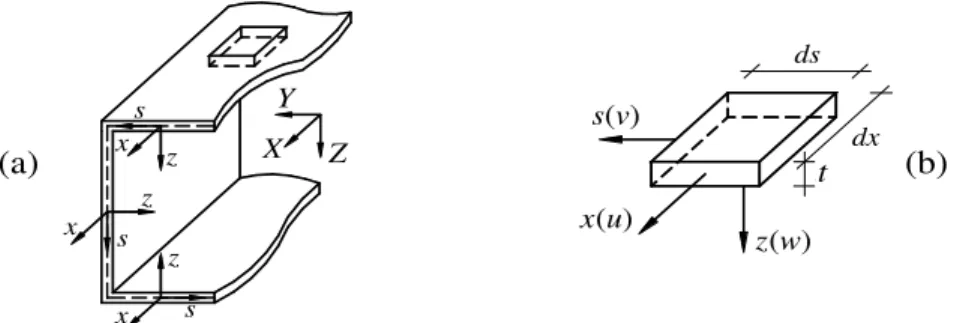
Consider the prismatic thin-walled member depicted in Figure 1(a), with a supposedly arbitrary cross-section and a global coordinate system _{𝑋 − 𝑌 − 𝑍}. Local coordinate systems _{𝑥 − 𝑠 − 𝑧} are adopted in each wall, as indicated in Fig. 1(b), where 𝑥(parallel to member longitudinal axis 𝑋) and 𝑠 define the wall mid-plane, and _𝑧 is measured along the wall thickness _𝑡. When expressed in this coordinate system, the displacement field components are termed _𝑈𝑥, _𝑈𝑠 and _𝑈𝑧.

x

x s s

z x

z z s

dx s(v)

x(u)

z(w) ds

X Y

Z

h

(a) _t (b)

Figure 1: (a) Prismatic thin-walled member with a supposedly arbitrary cross-section and global coordinate system, and (b) infinitesimal wall element with its local coordinate system and displacement components.

Adopting Kirchhoff’s hypothesis, which states that straight line segments/fibres normal to the mid-plane remain straight, inextensible and normal to the wall mid-plane after deformation (_{𝜀𝑧𝑧= 𝛾𝑥𝑧= 𝛾𝑧𝑥 = 𝛾𝑠𝑧 = 𝛾𝑧𝑠 = 0}), the displacement vector of an arbitrary point of the member, _{𝑈⃗⃗ (𝑥, 𝑠, 𝑧)}, is expressed as

𝑈⃗⃗ = {𝑈𝑈𝑥𝑠 𝑈𝑧

} = {𝑢 − 𝑧𝑤𝑣 − 𝑧𝑤,𝑥,𝑠

𝑤 } (1)

where (i) _{𝑢(𝑥, 𝑠)}, _{𝑣(𝑥, 𝑠)} and _{𝑤(𝑥, 𝑠)} are the mid-plane (_{𝑧 = 0}) displacement field components, and (ii) _(∙),𝑥=

𝜕 𝜕𝑥⁄ . The first terms of the in-plane displacement components (_𝑈𝑥 and _𝑈𝑠) stand for membrane displacements within the wall mid-plane, while the three remaining ones represent flexural displacements. In accordance with the classical thin-walled bar theory [38], the mid-plane displacement field can be conveniently expressed as (summation convention applies to subscript _𝑘)

𝑢(𝑥, 𝑠) = ∑𝑁𝑘=1𝑑 𝑢̅𝑘(𝑥, 𝑠)= 𝑢𝑘(𝑠)𝜑𝑘,𝑥(𝑥) (2a)

𝑣(𝑥, 𝑠) = ∑𝑁𝑘=1𝑑 𝑣̅𝑘(𝑥, 𝑠)= 𝑣𝑘(𝑠)𝜑𝑘(𝑥) (2b)

𝑤(𝑥, 𝑠) = ∑𝑁𝑘=1𝑑 𝑤̅𝑘(𝑥, 𝑠)= 𝑤𝑘(𝑠)𝜑𝑘(𝑥) (2c)

where (i) 𝑢_𝑘(𝑠), 𝑣_𝑘(𝑠) and 𝑤_𝑘(𝑠) are the mid-line functions defining cross-section deformation mode 𝑘 (or “GBT mode _𝑘”), (ii) _𝜑𝑘(𝑥) or _{𝜑𝑘,𝑥}(𝑥) are the amplitude functions describing their variation along the member length, (iii) _{𝑢̅𝑘(𝑥, 𝑠)}, _{𝑣̅𝑘(𝑥, 𝑠)} and _{𝑤̅𝑘(𝑥, 𝑠)} define the contribution of mode _𝑘 to the mid-plane displacement field and (iv) 1 ≤ 𝑘 ≤ 𝑁_𝑑, where 𝑁_𝑑 is the total number of deformation modes included in the analysis. Therefore, the member deformed configuration can be expressed as a sum of contributions from the 𝑁_𝑑 deformation modes  Eqs. (2a)-(2c) can also be written in matrix form as

𝑢 = 𝐮𝑇_𝛗

where (i) u, v and w are vectors containing the _𝑢𝑘(𝑠), _𝑣𝑘(𝑠) and _𝑤𝑘(𝑠) functions, respectively, and (ii) _𝛗 is a vector containing the corresponding amplitude functions _𝜑𝑘(𝑥) or _{𝜑𝑘,𝑥}(𝑥). Note that, for given deformation mode configurations, the longitudinal amplitude functions _𝜑𝑘(𝑥) fully define the member displacement field, comprising both the membrane and flexural components.

For a linear elastic material, following Hooke’s law for plane stress states, the member total strain energy is given by (_𝐿 is the member length)

𝑈 =₂1∫ (𝛗_𝐿 ,𝑥𝑥𝑇 𝐂𝛗,𝑥𝑥+ 𝛗,𝑥𝑇𝐃𝛗,𝑥+ 𝛗𝑇𝐁𝛗 + 𝛗𝑇,𝑥𝑥𝐄𝛗 + 𝛗𝑇𝐄𝑇𝛗,𝑥𝑥)𝑑𝑥 (4)

where _𝐂,_𝐁,_𝐃and_𝐄are (_{𝑁𝑑× 𝑁𝑑}) linear stiffness matrices, associated with (i) primary/secondary warping, (ii) transverse extension/flexure, (iii) plate shear distortion/torsion and (iv) membrane/flexural Poisson effects, respectively – their components are given by the expressions included in Appendix A.

The member is now considered subjected to a linear pre-buckling state, which is associated with a deformed configuration defined by the displacement components (see Eq. (3))

𝑢0_{= 𝐮}𝑇_𝛗 ,𝑥

0 _𝑣0_{= 𝐯}𝑇_𝛗0 _𝑤0_{= 𝐰}𝑇_𝛗0 ₍₅₎

where _𝛗0(𝑥), contains the amplitude functions quantifying the contributions of each of the _𝑁𝑑 GBT modes to that same deformed configuration. The pre-buckling stress field components – _𝜎𝑥𝑥0 (𝑥, 𝑠),

𝜎𝑠𝑠0(𝑥, 𝑠) and 𝜏𝑥𝑠0 (𝑥, 𝑠) − can then be expressed in a modal fashion, on the basis of 𝛗0(𝑥). The non-linear

(quadratic) term of the strain energy (_𝑈0) can be obtained by the work performed by those stresses on the corresponding quadratic components of strain [14], leading to

𝑈0₌1

2∫ ∑

(

𝛗,𝑥𝑇[𝐗𝑗σ−x𝜑𝑗,𝑥𝑥0 + 𝐗𝑗σ−xP𝜑𝑗0]𝛗,𝑥+ +𝛗𝑇_[𝐗

𝑗σ−sP𝜑𝑗,𝑥𝑥0 + 𝐗𝑗σ−s𝜑𝑗0]𝛗 + +𝛗𝑇_[𝐗

𝑗τ𝜑𝑗,𝑥0 ]𝛗,𝑥+ 𝛗𝑇,𝑥[(𝐗𝑗τ)𝑇𝜑𝑗,𝑥0 ] 𝛗) 𝑁𝑑

𝑗=1 𝑑𝑥

𝐿 (6)

where the three lines in the integrand involve geometrical stiffness terms associated with the _𝜎𝑥𝑥0 , _𝜎𝑠𝑠0 and

𝜏𝑥𝑠0 pre-buckling stress components, respectively. This means that 𝐗𝑗σ−x,𝐗𝑗σ−xP,𝐗𝑗σ−sP,𝐗𝑗σ−sand𝐗𝑗τ are

cross-section geometrical stiffness matrices associated with (i) normal longitudinal (_𝐗𝑗σ−x and_𝐗𝑗σ−xP), (ii) normal transverse (_𝐗𝑗σ−sP and_𝐗𝑗σ−s) and (iii) shear (_𝐗𝑗τ) pre-buckling stresses8_{– the analytical expressions} providing these matrices are included in Annex A.

To perform (linear) buckling analyses, the equilibrium equations can be obtained from the minimum total potential energy principle, which reads (_𝛿 stands for an infinitesimal variation)

𝛿(𝑈 + 𝑈0_{) = 0 ⇔}

⇔ ∫

(

𝛿𝛗,𝑥𝑥𝑇 𝐂𝛗,𝑥𝑥+ 𝛿𝛗,𝑥𝑇𝐃𝛗,𝑥+ 𝛿𝛗𝑇𝐁𝛗 + 𝛿𝛗,𝑥𝑥𝑇 𝐄𝛗 + 𝛿𝛗𝑇𝐄𝑇𝛗,𝑥𝑥+ +𝜆 ∑ {𝛿𝛗𝑁𝑗=1𝑑 𝑇,𝑥[𝐗𝑗σ−x𝜑𝑗,𝑥𝑥0 + 𝐗𝑗σ−xP𝜑𝑗0]𝛗,𝑥+

+𝛿𝛗𝑇_[𝐗

𝑗σ−sP𝜑𝑗,𝑥𝑥0 + 𝐗𝑗σ−s𝜑𝑗0]𝛗 + +𝛿𝛗𝑇_[𝐗

𝑗τ𝜑𝑗,𝑥0 ]𝛗,𝑥+ 𝛿𝛗,𝑥𝑇 [(𝐗𝑗τ)𝑇𝜑𝑗,𝑥0 ] 𝛗} )

𝑑𝑥 = 0

𝐿 (7)

where _𝜆 is the load parameter. Note that, at this stage, the _𝜑𝑗0(𝑥) functions (components of _𝛗0) have already been obtained by means of a (preliminary) pre-buckling analysis, performed for the loading under consideration. If the loadings cause only longitudinally uniform pre-buckling stress distribution (i.e.,

𝜎𝑥𝑥0 (𝑥, 𝑠) ≡ 𝜎(𝑠), 𝜎𝑠𝑠0 = 𝜏𝑥𝑠0 = 0), which is the case in this work, Eq. (7) becomes the weak form of

classical GBT of equilibrium equation (e.g., [1]),

⇔ ∫ (𝛿𝛗,𝑥𝑥

𝑇 _𝐂𝛗

,𝑥𝑥+ 𝛿𝛗,𝑥𝑇𝐃𝛗,𝑥+ 𝛿𝛗𝑇𝐁𝛗 + 𝛿𝛗,𝑥𝑥𝑇 𝐄𝛗 + 𝛿𝛗𝑇𝐄𝑇𝛗,𝑥𝑥+

+𝜆 ∑ {𝑊𝑁𝑗=1𝑑 𝑗𝛿𝛗,𝑥𝑇𝐗𝑗σ−x𝛗,𝑥} ) 𝑑𝑥 = 0

𝐿 (8)

where _𝑊𝑗 is the longitudinal normal stress resultant associated with mode _𝑗– in accordance with the typical GBT mode numbering criterion (see next section), only the first four terms (𝑗 = 1, … ,4) are usually considered: (i) _{𝑊1≡ 𝑁} (compressive axial force), (ii) _{𝑊2 ≡ 𝑀𝑌} (major-axis bending moment), (iii) _𝑊3≡

𝑀𝑍 (minor-axis bending moment) and (iii) 𝑊4≡ 𝑀𝜔 (torsion bi-moment). Carrying out integrations by

parts in _𝑥, and noting that _𝛿𝛗 is arbitrary, leads to the fourth-order differential equation system governing the linear eigenvalue buckling problem

𝐂𝛗,𝑥𝑥𝑥𝑥− 𝐃̃𝛗,𝑥𝑥+ 𝐁𝛗 − λ ∑ {𝑊𝑁𝑗=1𝑑 𝑗𝐗𝑗σ−x𝛗,𝑥𝑥}= 𝟎 (9)

where _𝐃̃ = 𝐃 + (𝐄 + 𝐄𝑇). In order to solve the above differential equation system, it is necessary to consider the corresponding boundary conditions

𝑾𝛿𝛗,𝑥|₀𝐿 with 𝑾 = 𝐂𝛗,𝑥𝑥+ 𝐄𝛗 (10a)

𝑾

̅̅̅𝛿𝛗|0𝐿 with 𝑾̅̅̅ = −𝐂𝛗,𝑥𝑥𝑥+ (𝐃 − 𝐄 − 𝜆𝑊𝑗𝐗𝑗σ−x)𝛗,𝑥 (10b)

where _𝑾 and _𝑾̅̅̅ stand for the cross-section resultants of the longitudinal and shear stresses, respectively. The determination of the components of the aforementioned tensors is made on the basis of the cross-section deformation modes, i.e., functions _𝑢𝑘(𝑠), _𝑣𝑘(𝑠) and _𝑤𝑘(𝑠), which are still unknown at this stage. These deformation modes are determined systematically, by means of a set of procedures termed “cross-section analysis”, which will be briefly described in the next section.

2.2 Cross-Section Analysis

As mentioned earlier, the first step of a GBT structural analysis is the determination of the cross-section deformation modes (i.e., functions _𝑢𝑘(𝑠), _𝑣𝑘(𝑠) and _𝑤𝑘(𝑠)) and the evaluation of the associated modal mechanical properties (the components of the tensors defined in Section 2.1), tasks that are performed through a systematic procedure termed Cross-Section Analysis. This work is based on a recently developed version of this procedure, applicable to arbitrary flat-walled members and described in detail in [6-7]  therefore, only a very brief overview is provided here.

It is necessary to begin by defining the cross-section nodal discretisation,which involves (i) natural internal nodes, (ii) natural end nodes and (iii) intermediate nodes [7]  while the first two sets of nodes are compulsory, the last one is optional and user-defined9_{. Three elementary deformation modes are associated} with each node, leading to a total of _{𝑁𝑑= 3 × 𝑁𝑛𝑜𝑑𝑒𝑠} elementary modes. Then, several linear stiffness matrices (_𝐂, _𝐁, _𝐃 and _𝐄) are calculated, on the basis of the above elementary modes, and subsequently used to perform a series of simultaneous diagonalisation operations. Such operations make it possible (i) to identify/separate deformation modes from different mechanical families and (ii) to arrange them, within

each family, according to a given hierarchy – one is led to a new set of (modal) “coordinates”: the _𝑁𝑑GBT deformation modes. The 3 main “mechanical families” involved are: (i) Vlasov modes, for which _{𝛾𝑥𝑠 = 𝜀𝑠𝑠=}

0, (ii) Shear modes, for which _{𝛾𝑥𝑠 ≠ 0; 𝜀𝑠𝑠= 0}, and (iii) Transverse Extension modes, for which _{𝜀𝑠𝑠 ≠ 0} each of these families can be further subdivided into several “deformation mode sub-families”.

For illustrative purposes, consider the lipped channel section displayed in Figure 2(a), which is discretised as shown in Figure 2(b). For the discretisation considered (involving 15 nodes), a total of 𝑁_𝑑 = 3 × 15 =

45 deformation modes are obtained  the in-plane or out-of-plane configurations of the most relevant ones are depicted in Figure 3. They comprise: (i) the four classical rigid-body (or “global”) modes (axial extension (1), major- and minor-axis bending (2-3) and torsion (4)), (ii) two distortional modes, associated with quasi-rigid body flange-lip motions (5-6), (iii) a sequence of local modes, involving transverse plate bending with increasing curvature (7-17), (iv) five global shear modes (18-22), consisting of the warping components of the Vlasov

modes 2-6, (v) a set of local shear modes, (23-31), (vi) five global transverse extension modes (32-36) and (vii)

the local transverse extension modes (37-45).

Depending on the particular problem under consideration, a selection of the GBT modes to be included in the structural analysis can be made, involving any sub-set of _𝑛𝑑 (_{1 ≤ 𝑛𝑑 ≤ 𝑁𝑑})  the solution is based exclusively on these selected modes. This Modal Selection capability makes it possible to (i) reduce the number of degrees of freedom involved in solving a problem and (ii) specify the nature of the deformation pattern(s) to be considered. In this work, only Vlasov modes are considered, as they suffice to accurately obtain buckling solutions of members acted by longitudinally uniform pre-buckling stresses.

3. GBT Member Analysis

After knowing the cross-section deformation modes and modal mechanical properties, it is possible to perform the Member Analysis, which provides the solution of the buckling problem under consideration, namely the set of _𝜑𝑘(𝑥) functions (_{1 ≤ 𝑘 ≤ 𝑛𝑑}) defining the member buckling mode shape.

In simply supported members, Eqs. (9) have an exact sinusoidal solution,

𝛗(𝑥) = 𝒂𝑠𝑖𝑛 (𝑛𝜋_𝐿 𝑥) (11)

where _𝒂 is a (_𝑛𝑑-dimension) vector containing the amplitudes of each modal amplitude function. This “analytical solution” is usually used because it minimises the number of degrees of freedom. For other support conditions a “numerical solution” must be used  this is usually done by discretising the member longitudinally into a mesh of conventional GBT-based finite elements.

3.1 GBT-based Conventional Finite Element

The variational statement expressed by Eq. (8) can be used to formulate and implement computationally a GBT-based beam conventional finite element. The main steps involved in these formulation and numerical implementation are described next:

(i) Approximate the longitudinal amplitude functions _{𝜑𝑘(𝑥)} (components of vector _𝛗(𝑥)) by means of linear combinations of cubic Hermite10 _{polynomials ℎ}

𝑖(𝜉), i.e.,

10 _{While Hermite polynomials could be used to approximate all the 𝜑}

(a) (b)

Figure 2: Lipped channel cross-section (a) geometry and (b) nodal discretization.

Figure 3: Lipped channel cross-section GBT deformation modes: (i) Vlasov modes (global (1-4), distortional (5-6) and local (7-17)), (ii) Shear modes (global (18-22) and local (23-31)) and (iii) Transverse Extension modes (isotropic (32)

and deviatoric (33-36) global, and local (37-45)). 𝑏𝑤= 100

𝑏𝑓= 60

𝑏𝑓= 60

𝑏𝑠= 10

(𝑡 = 2.0) 𝑚𝑚

𝑏𝑠= 10

𝛗(𝑥) = ℎ1(𝜉)𝒅1𝑒+ ℎ2(𝜉)𝒅2𝑒+ ℎ3(𝜉)𝒅3𝑒+ ℎ4(𝜉)𝒅4𝑒 (12)

where _{𝜉 = 𝑥 𝐿}⁄ _𝑒 (_𝐿𝑒 is the element length) and the polynomials read

ℎ1(𝜉) = 𝐿𝑒(𝜉3− 2𝜉2+ 𝜉) ℎ2(𝜉) = 2𝜉3− 3𝜉2+ 1 ₍₁₃₎

ℎ3(𝜉) = 𝐿𝑒(𝜉3− 𝜉2) ℎ4(𝜉) = −2𝜉3+ 3𝜉2

Vectors _𝒅𝑖𝑒 contain the element degrees of freedom, i.e., the nodal values and derivatives of the amplitude functions: _𝒅1𝑒_{≡ 𝛗,𝑥}(0), _𝒅2𝑒_{≡ 𝛗(0)}, _𝒅3𝑒_{≡ 𝛗,𝑥}(1) and _𝒅4𝑒_{≡ 𝛗(1)} – because there are _𝑛𝑑 amplitude functions, the element exhibits a total of _{4 × 𝑛𝑑} degrees of freedom.

(ii) Incorporate Eqs. (12)-(13) into Eq. (8) and carry out the corresponding integrations (over 𝐿_𝑒), in order to obtain the finite element linear and geometrical stiffness matrices

𝐊𝑒_{= 𝐂 ⊗ 𝐤} 22

𝑒 _{+ 𝐃 ⊗ 𝐤}

11𝑒 + 𝐁 ⊗ 𝐤00𝑒 + 𝐄 ⊗ 𝐤20𝑒 + 𝐄𝑇⊗ 𝐤02𝑒 (14)

𝐆𝑒_{= ∑ {𝑊}

𝑗𝐗𝑗σ−x} 𝑁𝑑

𝑗=1 ⊗ 𝐤11𝑒 (15)

where “⊗” denotes the tensor product and the 4 × 4 matrices _𝐤𝑖𝑗𝑒 (_𝑖 and _𝑗 are the orders of derivation of the two functions involved) are given by

𝐤00𝑒 =₄₂₀𝐿𝑒

[

4𝐿2𝑒 22𝐿𝑒 −3𝐿2𝑒 13𝐿𝑒

22𝐿𝑒 156 −13𝐿𝑒 54

−3𝐿2𝑒 −13𝐿𝑒 4𝐿2𝑒 −22𝐿𝑒

13𝐿𝑒 54 −22𝐿𝑒 156 ]

[

4𝐿2𝑒 3𝐿𝑒 −𝐿𝑒2 −3𝐿𝑒

3𝐿𝑒 36 3𝐿𝑒 −36

−𝐿2𝑒 3𝐿𝑒 4𝐿2𝑒 −3𝐿𝑒

−3𝐿𝑒 −36 −3𝐿𝑒 36 ]

(16a)

𝐤22𝑒 =_𝐿2_𝑒3

[

2𝐿2𝑒 3𝐿𝑒 𝐿2𝑒 −3𝐿𝑒

3𝐿𝑒 6 3𝐿𝑒 −6

𝐿2𝑒 3𝐿𝑒 2𝐿2𝑒 −3𝐿𝑒

−3𝐿𝑒 6 −3𝐿𝑒 6 ]

[

−4𝐿2𝑒 −33𝐿𝑒 𝐿2𝑒 3𝐿𝑒

−3𝐿𝑒 −36 −3𝐿𝑒 36

𝐿2𝑒 −3𝐿𝑒 −4𝐿2𝑒 33𝐿𝑒

3𝐿𝑒 36 3𝐿𝑒 −36]

𝐤02𝑒 = (𝐤20𝑒 )𝑇 (16b)

(iii) Take into account the member end support conditions, expressed in terms of the GBT modal degrees of freedom, and assemble the finite element matrices to obtain the (discretised) eigensystem

(𝐊 − λ𝐆)𝐚 = 𝟎 (17)

where 𝑲, and 𝑮 denote the member overall linear and geometrical stiffness matrices, and 𝐚 (eigenvector) provides the buckling mode configuration expressed in terms of the finite element degrees of freedom. An upper bound on the system dimension is _{2𝑛𝑑(𝑛𝑓𝑒+ 1)}, where _𝑛𝑓𝑒 is the number of finite elements. 3.2 GBT-Based Exact Element Approach

The implementation of the exact element is now presented. It involves two main steps: (i) expressing the modal amplitude functions as power series and finding their coefficients, and (ii) deriving the exact elementary non-linear stiffness matrix.

3.2.1 Expression of 𝝋(𝑥) as a power series

As a first step, GBT differential equilibrium equations system are normalized using _{𝑥 = 𝜉𝐿} and, therefore, Eqs. (9) can be written as

𝛗,𝜉𝜉𝜉𝜉− 𝐃𝛗,𝜉𝜉+ 𝐁𝛗 + λ𝐗𝛗,𝜉𝜉= 𝟎 (18)

𝐃 = 𝐿2_𝐂−1_{𝐃̃ (19a)}

𝐁 = 𝐿4_𝐂−1_{𝐁 (19b)}

𝐗 = 𝐿2_𝐂−1_{∑ {𝑊} 𝑗𝐗𝑗σ−x} 𝑁𝑑

𝑗=1 (19c)

It should be noted that matrix _𝐂 is always invertible in the modal space under consideration, since the conventional Vlasov modes always involve non-null primary and/or secondary warping stiffness. In addition, the above calculations need to be performed only once, because the matrices are constant throughout the process. Then, _𝛗(𝜉) (solution of the problem) can be written as a power series

𝛗(𝜉) = ∑

𝒇

𝜉

where {𝒇_{0, … , 𝒇∞}} are the coefficient vectors (_𝑛𝑑-dimension), and the substitution of Eq. (20) into Eq. (18) yields

∑(𝑛 + 4)!_𝑛! 𝒇𝑛+4 ∞

𝑛=0

𝜉𝑛_{− 𝐃 ∑}(𝑛 + 2)!

𝑛! 𝒇𝑛+2

∞

𝑛=0

𝜉𝑛_{+ 𝐁 ∑ 𝒇} 𝑛 ∞

𝑛=0

𝜉𝑛₊

+𝜆𝐗 ∑(𝑛 + 2)!_𝑛! 𝒇𝑛+2 ∞

𝑛=0

𝜉𝑛 _{= 𝟎}

(21)

This equation is satisfied for any value of _𝜉 if and only if all the terms with the same power _𝑛 are equal to zero, i.e.,

(𝑛+4)!

𝑛!

𝒇

−

(𝑛+2)!

𝑛!

𝐃𝒇

+ 𝐁𝒇

+ 𝜆𝐗

(𝑛+2)!

𝑛!

𝒇

= 𝟎

which constitutes a linear homogeneous recursive formula: each term is dependent on the four preceding ones for each of the _𝑛𝑑 deformation modes. Finally, Eq. (22) can be simplified to read

𝒇

= 𝑎

𝐃̅

𝒇

− 𝑏

𝐁𝒇

where _𝐃̅_𝜆 is a non-linear stiffness matrix given by

𝐃̅

= 𝐃 − 𝜆𝐗

and _𝑎𝑛 and _𝑏𝑛 are series given by

𝑎

=

𝑏

=

(25)

By assigning values to (i) parameter11_{𝜆, and (ii) the first four coefficients {𝒇}

0, … , 𝒇3}, Eq. (22) makes it

possible to find the remaining coefficients in the series, _{{𝒇4, … , 𝒇∞}}, and therefore, obtain an exact solution to the differential equilibrium equation system – one that, in general, does not verify the member boundary conditions (Eqs. 9(a)-(b)). On the other hand, it is not practical to adopt coefficients {𝒇₀, … , 𝒇₃} as the element degrees of freedom (they do not have an obvious physical meaning)  instead, it is preferable to adopt the degrees of freedom of the conventional finite element, (nodal values and derivatives of the modal amplitude functions): _𝒅1𝑒 _{≡ 𝛗,𝑥}(0), _𝒅2𝑒_{≡ 𝛗(0)}, _𝒅3𝑒_{≡ 𝛗,𝑥}(1), _𝒅4𝑒_{≡ 𝛗(1)}, which leads to (see Eq. (12)),

𝛗(𝑥) = 𝐄1(𝜉)𝒅1𝑒+ 𝐄2(𝜉)𝒅2𝑒+ 𝐄3(𝜉)𝒅3𝑒+ 𝐄4(𝜉)𝒅4𝑒 (26)

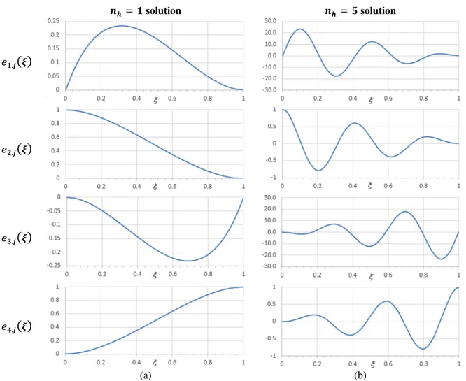
where the four _𝐄𝑖(_{𝑛𝑑× 𝑛𝑑}) matrices contain the exact shape functions associated with the four types of degrees of freedom. A striking difference with respect to Eq. (12) is the fact that the shape functions must now be expressed by matrices, whose components are interpreted as follows:

(i) The diagonal components, 𝐸_𝑖(𝜉) _𝑗𝑗 = 𝑒_𝑖.𝑗(𝜉), are directly associated with the imposed displacements – thus, _{𝑒𝑖.𝑗}(𝜉) is the shape function of the _𝑗-th mode stemming from imposing a unit value on its own _𝑖-th degree of freedom (displacement or derivative). Figures 4(a)-(b) show the 4 basic function types (_{𝑖 = 1, … ,4}) for two solutions: one involving a single half-wave (_{𝑛ℎ= 1}, see Fig. 4(a)) and the other involving five half-waves (_{𝑛ℎ= 5}, see Fig. 4(b)).

𝒏𝒉= 𝟏 solution 𝒏𝒉= 𝟓 solution

𝒆𝟏.𝒋

(𝝃)

𝒆𝟐.𝒋

(𝝃)

𝒆𝟑.𝒋

(𝝃)

𝒆𝟒.𝒋

(𝝃)

(a) (b)

Figure 4: Exact finite element shape functions associated with the 4 degrees of freedom of a given deformation mode _𝑗– solutions involving (a) a single half-wave (_{𝑛ℎ= 1}) and (b) five half-waves (_{𝑛ℎ = 5}).

Hence, this exact finite element involves the same _{4 × 𝑛𝑑} degrees of freedom as the conventional one. However, it also has _{4 × 𝑛𝑑}2 exact shape functions (the components of the four _𝐄𝑖(𝜉) matrices), which must be determined. In the next section, the systematic procedure adopted to determine these functions is addressed. 3.2.2 Power Series and Boundary Values/Derivatives

Before addressing the determination of the exact finite element shape functions and non-linear stiffness matrix, it is useful to investigate the mathematical relations between the power series terms and the values of the amplitude functions _𝛗(𝜉), and their derivatives, at the element ends/nodes (_{𝜉 = 0}, ₁). From Eq. (20) it follows that

𝛗(0) = ∑ 𝒇𝑛𝜉𝑛 ∞

𝑛=0 |

𝜉=0

= 𝒇0 (27)

𝛗(1) = ∑ 𝒇𝑛𝜉𝑛 ∞

𝑛=0 |

𝜉=1

= ∑ 𝒇𝑛 ∞

𝑛=0

(28)

As shown by Eq. (27), the value of the amplitude function at _{𝜉 = 0} is equal to a single coefficient of the series (𝛗(0) ≡ 𝒇₀), a statement that can be extended to its derivatives – i.e., for the 𝑚-th order derivative, one has

𝛗(𝑚)(0) = 𝑚! 𝒇𝑚 (29)

On the other hand, Eq. (28) shows that the value of the amplitude function at _{𝜉 = 1} is given as a sum involving all the terms of the series. However, since a linear fourth-order series is involved, all the terms depend, in this particular case, exclusively on the first four terms (_𝒇0 to _𝒇3) and, therefore, _𝛗(1) can be more conveniently expressed as

𝛗(1) = 𝐀00𝒇0+ 𝐀01𝒇1+ 𝐀02𝒇2+ 𝐀03𝒇3 (30)

where the (_{𝑛𝑑× 𝑛𝑑}) matrices _𝐀0_𝑘can be obtained by means of

[𝐀0𝑘]_𝑖𝑗 = ∑∞𝑛=0[𝒇̃𝑛]_𝑖 (31)

in which ∙ _𝑖𝑗 stands for the _{(𝑖, 𝑗)} tensorial component and _𝒇̃𝑛 are the coefficients of an auxiliary power series obtained by using Eq. (22), with its first four terms (_𝒇̃0 to _𝒇̃3) being given by

[𝒇̃𝑙]_𝑗= 𝛿𝑘𝑙 (32)

where _𝛿𝑘𝑙 is the Kronecker delta (_{𝑘, 𝑙 = 0,1,2,3}). Then, for a given power series with coefficients

{𝒇0, … , 𝒇∞}, Eq. (30) makes it possible to obtain the end displacement as a function of only the first four

of them ({𝒇₀, … , 𝒇₃}). Note that the superscript “0” appearing in the above matrices indicates that the expression provides the end value of the _𝛗(𝜉) function – for the _𝑚-th order derivative, Eqs. (30)-(31) become

𝛗(𝑚)(1) = 𝐀𝑚0𝒇0+ 𝐀𝑚1𝒇1+ 𝐀𝑚2𝒇2+ 𝐀𝑚3𝒇3 (33)

while Eq. (32) still applies to provide _{{𝒇̃0, … , 𝒇̃3}}. Although the determination of the 16 matrices _𝐀𝑚_𝑘 (_{𝑘, 𝑚 = 0,1,2,3}) is indispensable to carry out the procedure addressed in the next section, it can be performed beforehand and independently of it.

3.2.3 Derivation of the Exact Element Shape Functions and Non-Linear Stiffness Matrix

For a GBT buckling analysis involving _𝑛𝑑 deformation modes, the exact element non-linear stiffness matrix has dimension _{4𝑛𝑑× 4𝑛𝑑}, since the differential equilibrium equations include fourth-order derivatives. Its entries are theboundarytermvalues,namely_𝑾𝑖(0), _𝑾̅̅̅_𝑖(0), _𝑾𝑖(1)and_𝑾̅̅̅_𝑖(1) (_{1 ≤ 𝑖 ≤ 𝑛𝑑},seeEqs. (10(a)-(b)), which are evaluated on the basis of the _{4 × 𝑛𝑑} shape functions associated with the element degrees of freedom (amplitude function values and derivatives at the ends/nodes). This procedure involves the following steps:

(i) ForaGBTmode _𝑗, a unitarydisplacementorderivativeis imposed to each of its degrees of freedom – in order to obtain the ensuing shape functions as power series, the first four coefficient vectors {𝒇_{0, … , 𝒇3}} must be determined. While the first two (_𝒇0 and 𝒇₁) can be readily obtained from the boundary conditions (see Table 1), the remaining two (_𝒇2 and 𝒇₃) must be evaluated by solving the _{2 × 𝑛𝑑} linear system

{𝐀2 0_𝒇

2+ 𝐀03𝒇3= 𝝋(1) − 𝐀00𝒇0− 𝐀01𝒇1 𝐀12𝒇2+ 𝐀13𝒇3= 𝝋,𝜉(1) − 𝐀11𝒇1

(35)

where _𝝋(1) and _𝝋,𝜉(1) are the values and derivatives of the shape functions at the end node, which can be straightforwardly obtained from the boundary conditions (see Table 1). The set of four coefficient vectors _{{𝒇0, … , 𝒇3}} obtained, as described above, for the _𝑖-th degree of freedom of mode

𝑗 make it possible to determine the 𝑗-th column of matrix 𝐄_𝑖(𝜉) – repeating the procedure for all modes leads to the complete definition of the matrices appearing in Eq. (26).

Table 1: Vectors _𝒇0, _𝒇1, _𝝋(1) and _𝝋,𝜉(1) for the various shape functions (vector {𝟏} has unit components).

𝒇₀ 𝒇₁ 𝝋(1) 𝝋_,𝜉

(1)

𝑒1.𝑗

(𝜉)

{𝟏}

𝑒2.𝑗

(𝜉)

{𝟏}

𝑒3.𝑗

(𝜉)

{𝟏}

𝑒4.𝑗

(𝜉)

{𝟏}

𝐄

(𝜉)

(ii) The boundary forces (_𝑾𝑖(0), _𝑾̅̅̅_𝑖(0), _𝑾𝑖(1), _𝑾̅̅̅_𝑖(1)) are determined using Eqs. (10(a)-(b)) on the basis of the shape functions, namely their first 4 coefficients. For terms involving higher-order derivatives (_{𝑚 = 2,3}), Eq. (33) can be employed.

4. Illustrative Examples

The application and performance of the exact GBT-based finite element just presented are now considered. The numerical illustrative examples presented and discussed in the next subsections concern cold-formed steel lipped channel columns with the cross-section dimensions given in Figure 2(a) and material properties _{𝐸 = 210𝐺𝑃𝑎} and _{𝜈 = 0.3} since the loading consists of uniform axial compression _𝑁, one has _{∑ {𝑊}𝑁𝑑 _𝑗𝐗𝑗σ−x_}

𝑗=1 ≡ 𝑁𝐗1σ−x. The buckling behaviour of such columns is assessed by means of GBT analyses

employing either “analytical solutions” (“AS”), conventional based finite elements (“CE”) or exact GBT-based elements (“EE”), with the objective of comparing the three sets of results – note that the first two sets of results are obtained by means of program GBTUL [24], while the last one stems from a FORTRAN code written specifically to implement the “EE” approach.

4.1 Simply Supported Columns  Validation

In order to validate the numerical implementation of the exact finite element, the buckling behaviour of simply supported12 _{columns is first considered. Figure 5(a) depicts (i) a curve 𝜆 − 𝐿 providing the variation of} the column critical buckling load with its length, obtained though GBT “analytical solutions”13 _{and (ii) eight buckling} loads, obtained with exact (“EE”) GBT-based elements and identified by circles. The fact that the two sets of buckling loads values virtually coincide (differences below 0.05%), irrespective of column length and nature of the buckling mode, provides clear evidence that the GBT exact element was adequately implemented. As expected, a similar buckling load coincidence takes place when only fractions of the whole deformation mode

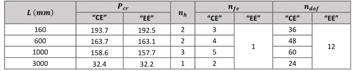
Table 2: Comparison between similarly accurate “CE” and “EE” analyses: critical buckling loads (_𝑃𝑐𝑟) and numbers of finite elements (_𝑛𝑓𝑒) and degrees of freedom (_{𝑛𝑑𝑜𝑓}) required to obtain them.

𝑳 (𝒎𝒎) _“CE” 𝑷𝒄𝒓 _“EE” 𝒏𝒉 _“CE” 𝒏𝒇𝒆 _{“EE” “CE”} 𝒏𝒅𝒐𝒇 _“EE”

160 193.7 192.5 2 3

1

36

12

600 163.7 163.1 2 4 48

1000 158.6 157.7 3 5 60

3000 32.4 32.2 1 2 24

12 _{In the GBT modal terminology, “simply supported” means that the deformation mode amplitude functions have null nodal} values, while the corresponding derivatives are kept as degrees of freedom  i.e., _{𝛗(0) = 𝛗(1) = 0}.

(a)

(b)

(c)

(a)

(b)

(c)

(d)

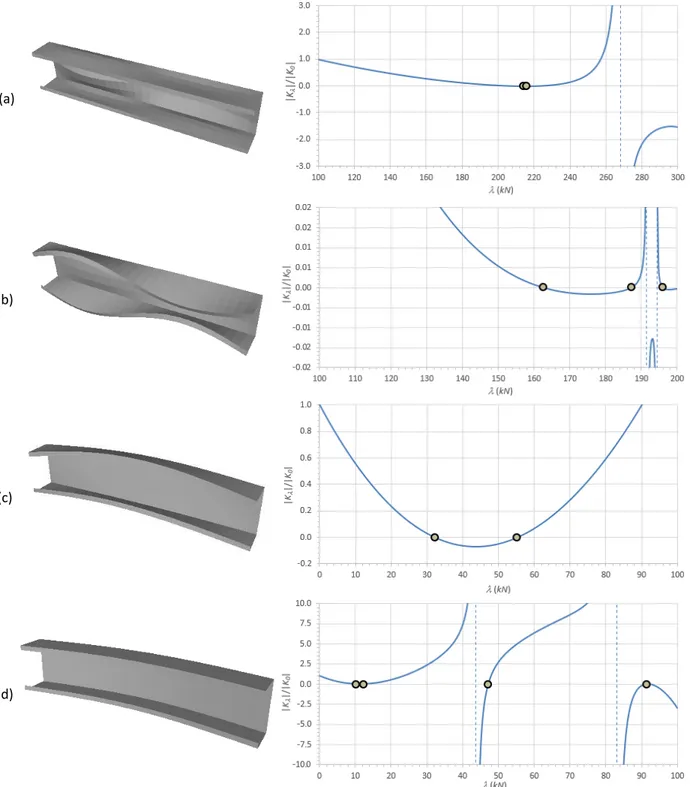
Figure 6: Lipped channel critical buckling mode fundamental shapes (depicted to the same longitudinal scale) and |𝐊𝜆| |𝐊⁄ 0| vs. 𝜆 curves (indicating the first roots in the interval shown): (a) 𝐿 = 120𝑚𝑚, (b) 𝐿 = 600𝑚𝑚, (c) 𝐿 =

4000𝑚𝑚 and (d) _{𝐿 = 7000𝑚𝑚} columns.

5(c) displays the modal participation diagram, which shows the variation of the critical buckling mode nature with the column length. It can be observed that the column critical buckling mode is (i) local (mode

7 prevails  see Fig. 6(a)), for _{𝐿 ≤ 200𝑚𝑚}, (ii) distortional (mode 5 prevails  see Fig. 6(b)), for _{200 < 𝐿 <}

1200𝑚𝑚, (iii) flexural-torsional (modes 2 and 4 see Fig. 6(c)) or (iv) flexural (mode 3 see Fig. 6(d)), for _{𝐿 ≥}

6000𝑚𝑚. The modal participation diagram agrees with Figure 5(b), in the sense that a few deformation modes suffice to obtain exact results in certain length ranges.

Finally, Figures 6(a)-(d) show the buckling mode shapes mentioned in the previous paragraph and also curves depicting the variation of the normalised non-linear stiffness matrix determinant (|𝐊_𝜆| |𝐊⁄ ₀|) with the load parameter for 4 column lengths: _{𝐿 = 120𝑚𝑚}, _{𝐿 = 600𝑚𝑚}, _{𝐿 = 4000𝑚𝑚} and _{𝐿 = 7000𝑚𝑚}, showing the first roots, providing the lower buckling load values and mode shapes of each column.

Next, in order to make a first assessment of the degree of freedom economy associated with the use of the “exact element” approach, with respect to the “conventional element” one, the columns having lengths 𝐿 = {160, 600, 1000, 3000} 𝑚𝑚 are also analysed by means of the “CE” approach, discretising the columns into 2 to 5 finite elements, which are the lowest numbers required to achieve virtually exact results (i.e., _𝑃𝑐𝑟 differences below _1%). In both cases, the GBT analyses include modes {𝟐, 𝟒, 𝟓, 𝟔, 𝟕, 𝟗}. Table 2 shows a comparison between the results obtained with the “CE” and “EE” approaches, as well as the numbers of degrees of freedom involved in performing the two sets of GBT buckling analyses. Note that a single exact element involves

𝑛𝑑𝑜𝑓= 12 degrees of freedom14, while equally accurate analyses using conventional finite elements require

between 24 and 60 degrees of freedom, depending on the number of half-waves exhibited by buckling mode (_𝑛ℎ): obviously, a higher _𝑛ℎ requires a finer “CE” mesh (i.e., more degrees of freedom) to provide results as accurate as those obtained with a single “EE”.

4.2 Columns with Other Support Conditions

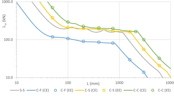
Figure 7 provides _{𝜆 − 𝐿} curves for columns other than simply supported, namely exhibiting the following end support conditions: (i) clamped-free15 (“C-F” _ cantilever), (ii) clamped-simply supported (“C-S”) _{and (iii)} clamped-clamped (“C-C”). They were obtained by means of the “CE” approach, including the same set of deformation modes considered earlier ({𝟐, 𝟒, 𝟓, 𝟔, 𝟕, 𝟗}) and discretising the columns into the minimum numbers of conventional finite elements required to obtain “exact” buckling results.

The circles identify again the buckling loads determined with the “EE” approach  note that it was necessary to consider two exact finite elements in the C-C columns, due to the fact that a single finite element would have all its degrees of freedom fully constrained. It is observed that, once more, there is a virtual coincidence between the buckling loads provided by the “CE” and “EE” approaches – all the differences are below 0.02%. For _{𝐿 =}

{160, 600, 1000, 3000} 𝑚𝑚, Table 3 presents and compares the critical buckling loads _𝑃𝑐𝑟 provided by both methods and the numbers of finite elements and degrees of freedom required to obtain them. It is observed that, in order to achieve similar accuracy, the numbers of degrees of freedom required by the “CE” approach is 2 to 10 times larger than those associated with the use of the exact element method.

14 _{To be completely fair, it should be recalled that, unlike its conventional finite element counterpart, the exact element} approach requires the a priori preliminary definition of the exact shape functions, i.e., the determination of the power series coefficients (Eq. (23)). The maximum number of coefficients (i.e., the power series order) that was necessary to obtain accurate buckling loads, up to the machine precision, was found to be usually in the 40-60 range  however, it can be over 100 is some (rare) cases.

4.3 Conventional vs. Exact Elements: Comparison

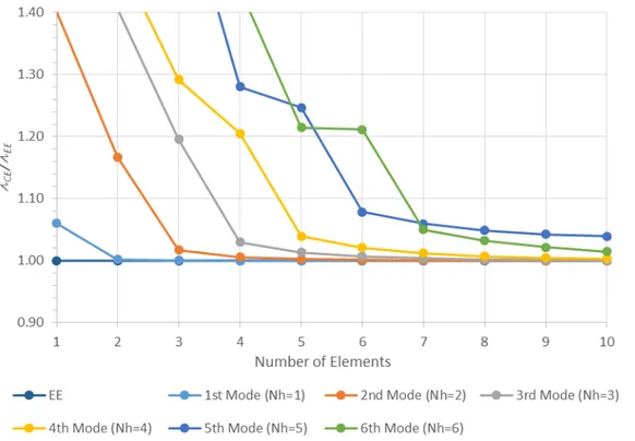
The performances of the exact and conventional (finite) elements are now compared. Figure 8 shows the variation of the buckling load ratio _{𝜆𝐶𝐸⁄𝜆𝐸𝐸} concerning a simply supported column with length _{𝐿 = 400𝑚𝑚} and buckling in pure symmetric distortional modes (i.e., only mode 5 is included in the GBT analyses)

exhibiting between one and six half-waves (𝑁_ℎ= 1, … ,6). In other words, they are the first six buckling modes of the above column when it is “restrained” to exhibit only symmetric distortional deformations. Naturally, the exact element approach provides the same buckling load regardless of the numbers of elements and buckling mode half-waves. Conversely, the buckling loads obtained by means of the conventional finite element approach decrease as the number of finite elements increases, for every buckling mode half-wave number  in general, exact buckling loads are reached when 2-3 conventional finite elements are considered per buckling mode half-wave. Therefore, the “degree of freedom economy” associated with the use of the “EE” approach, with respect to the “CE” one, increases with the buckling mode half-wave number16_.

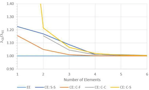
Similarly, Figure 9 plots _𝜆𝐶𝐸⁄_𝜆𝐸𝐸 against the number of finite elements, for _{𝐿 = 1000𝑚𝑚} columns with the four different end support conditions dealt with in this work (S-S, C-F, C-C and C-S). It can be observed that the accuracy of the solution provided by the conventional finite element approach increases differently with the number of finite elements for the various columns (and the associated buckling mode natures). For instance, using a single conventional finite element leads to a strong overestimation of the C-S column buckling load (_{𝜆𝐶𝐸⁄𝜆𝐸𝐸 ≈ 6})  indeed, it is necessary to consider 5 finite elements to obtain a virtually exact solution (error below 1%). As for the C-C column, which requires 2 exact elements to obtain the solution, it ends up being the one requiring the highest number of conventional finite elements to achieve accuracy  in the cantilevered column, 3 conventional finite elements are sufficient to attain that same goal.

Another advantage of the exact element approach stems from the fact that the modal amplitude functions, as well as their derivatives, are provided (approximated) by single analytical expressions along the whole column/member length  instead of approximations by means of piecewise cubic (or of a lesser order)

Figure 7: _{𝜆 − 𝐿} curves for S-S, C-F, C-S and C-C columns.

16_{Recall that, as stated in footnote 9, a “fair comparison” must also consider the number of coefficients involved in the exact} shape functions  this number tends to increase as the support conditions become “more restrained”.

10.0 100.0 1000.0

10 100 1000 10000

lcr

(kN

)

L (mm)

Table 3: Comparison between the “CE” and “EE” analyses for C-F, C-C and C-S columns: critical buckling loads (_𝑃𝑐𝑟) and numbers of finite elements (_𝑛𝑓𝑒) and degrees of freedom (_{𝑛𝑑𝑜𝑓}) required to obtain them.

𝑳 (𝒎𝒎) _“CE” 𝑷𝒄𝒓 _{“EE” “CE”} 𝒏𝒇𝒆 _{“EE” “CE”} 𝒏𝒅𝒐𝒇 _“EE”

C-F

160 94.8 94.3 2

1

24

12

600 82.1 81.7 4 48

1000 59.4 59.4 3 36

3000 13.8 13.8 3 36

C-C

160 244.3 242.5 5

2

48

12

600 198.3 197.7 7 72

1000 184.9 183.9 6 60

3000 100.6 99.8 3 24

C-S

160 197.6 196.6 4

1

42

6

600 180.8 179.7 4 42

1000 165.8 164.6 5 54

3000 55.6 55.4 6 66

polynomials associated with the conventional finite element approach. In order to illustrate the above assertion, Figure 10 shows, for the column under consideration, the mode 5 amplitude functions (𝜑(𝑥)) and their second derivatives (_{𝜑,𝑥𝑥}(𝑥)), required to determine the longitudinal stress distributions, concerning the “pure” distortional buckling modes with 1, 3 and 5 half-waves. The results presented were obtained using (i) 1 exact element and (ii) 3 conventional finite elements – since the latter adopt cubic polynomials as approximation functions, the corresponding _{𝜑,𝑥𝑥}(𝑥) functions are piecewise linear.

Figure 9: Variation of _{𝜆𝐶𝐸⁄𝜆𝐸𝐸} with the number of conventional and exact finite elements for the critical buckling mode of a _{𝐿 = 1000𝑚𝑚} column for different support conditions: S-S, C-F, C-C and C-S.

𝝋(𝒙) 𝝋,𝒙𝒙(𝒙)

(a)

(b)

(c)

The plots on the left hand side conform what is well known: the 3 conventional elements provide quite good approximations of the exact (sinusoidal17_{) amplitude functions  although the quality of the} approximation decreases with _𝑁ℎ, it is fairly good even for _{𝑁ℎ= 5}. Conversely, the exact second derivatives of the above amplitude functions are approximated (linearly) in a much poorer fashion, regardless of the

𝑁ℎ value – for 𝑁ℎ= 3 and 𝑁ℎ= 5, the maximum values are significantly under- and overestimated,

respectively. This level of approximation can only be improved by increasing significantly the number of (conventional) finite elements. Since, as mentioned before, the longitudinal stress distributions associated with a given buckling mode, are proportional to _{𝜑,𝑥𝑥}(𝑥), accurate (multi-linear) representations of the stress field can only be achieved by adopting a very fine conventional finite element mesh  on the contrary, a single exact element leads to an excellent (smooth) approximation of both _{𝜑,𝑥𝑥(𝑥)} and the stress field.

4.4 Exact Element Limitations

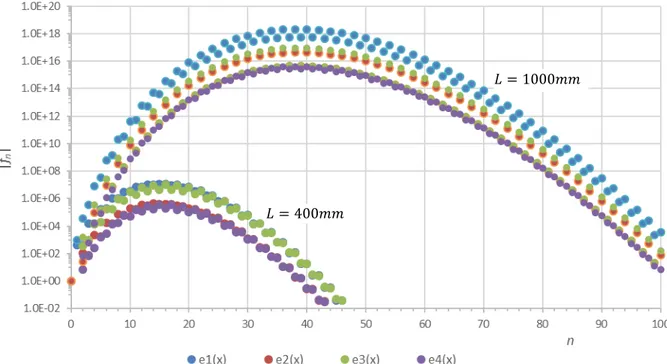
It was found that the solution of buckling problems by means of the exact element approach may become numerically unstable for long columns (𝐿 > 800𝑚𝑚) buckling in local modes (e.g., modes {7,9}. This is due to the large half-wave numbers involved, which leads to polynomials with very high orders, and also to the fact that local modes exhibit very small warping stiffness (in comparison with those of global or distortional modes). The above two features are responsible for the fact that the recursive formula (Eq. (22)), which is based on the inversion of matrix _𝐂 (Eqs. (18a-c)), provides series of coefficients with reversing signs (_{𝑠𝑔𝑛(𝑓𝑛}) = −𝑠𝑔𝑛(𝑓_𝑛−1)) and very high values (prior to the vanishing of the corresponding absolute values). Figure 11 illustrates this assertion, by showing the absolute values of the coefficients defining the four exact element shape functions (plots _|𝑓𝑛|vs.𝑛) for simply supported columns with (i) _{𝐿 = 400𝑚𝑚} and (ii) _{𝐿 = 1000𝑚𝑚},whichare “forced” to buckle in mode

7. It is observed that, for the _{𝐿 = 1000𝑚𝑚} column, it is

Figure 11: Absolute values of the series coefficients defining the 4 exact element shape functions for the analysis of S-S columns with (i) _{𝐿 = 400𝑚𝑚} and (ii) _{𝐿 = 1000𝑚𝑚}and “forced” to buckle in mode 7𝜆 = 159.9 𝑘𝑁.

17The polynomial approximations provided by the exact element approach are virtual “exact”, although, naturally, the number of coefficients that have to be considered grows fast with the number of buckling mode half-waves.

𝐿 = 400𝑚𝑚

necessary to calculate coefficients of orders higher than 100 (_{𝑛 > 100}), which can exhibit absolute values above 1018 _(|𝑓

𝑛| > 1018)  these values are many more and much higher than those concerning the 𝐿 = 400𝑚𝑚

column (_{𝑛 < 50, |𝑓𝑛| < 10}8). This fact leads to a very error-prone situation, due to the inaccuracy of the stiffness matrix and an unstable (oscillating) determinant curve. This difficulty could possibly be circumvented either (i) by neglecting the warping stiffness all together (𝐂 ≈ 𝟎), which would lead to an alternative (second-order) form of the recursive formula and should not entail significant errors, or (ii) by considering more than one exact element.

6. Conclusion

This paper presented the formulation, implementation and application of an exact GBT-based beam element intended for the buckling analysis of thin-walled members, namely columns. This element, which is “exact” up to machine precision, approximates the modal longitudinal amplitude functions by means of power series whose coefficients are provide by a fourth-order recursive formula. The buckling loads, and corresponding mode shapes, are obtained by finding the roots of the determinant of the ensuing non-linear stiffness matrix (which is a function of the load parameter _𝜆).

The performance quality of the exact element was investigated by means of a few illustrative numerical examples concerning lipped channel columns, which validated the implementation carried out and also compared the results obtained by means of the proposed approach with those provided by the conventional GBT-based finite element approach, which uses cubic Hermite polynomials as shape functions. This comparison showed that the exact element approach provides virtually “exact” results, thus validating its implementation, while minimising the number of degrees of freedom involved in the analysis and eliminating the need for a longitudinal mesh  the increased efficiency of the exact element approach, with respect to its conventional finite element counterpart, is naturally higher for columns buckling in modes exhibiting large half-wave numbers. On the other hand, it was also found that, in long columns buckling locally, numerical instabilities may prevent the proposed approach to provide accurate results  however, it seems that this difficulty can be fairly easily circumvented.

Annex A

The components of the GBT cross-section linear and geometrical stiffness matrices read

𝐶

= ∫

𝑢

𝑢

𝑑𝑠

+ ∫

𝐸𝑡3

12(1−𝜈2₎

𝑤

𝑤

𝑑𝑠

𝑆 (36a)

𝐵

= ∫

𝑣

𝑣

𝑑𝑠

+ ∫

𝐸𝑡3

12(1−𝜈2₎

𝑤

𝑤

𝑑𝑠

𝑆 (36b)

𝐷

= ∫ 𝐺𝑡(𝑢

+ 𝑣

)(𝑢

+ 𝑣

)𝑑𝑠

+ ∫

3

3

𝑤

𝑤

𝑑𝑠

𝑆 (36c)

𝐸

= ∫

𝑢

𝑣

𝑑𝑠

+ ∫

𝜈𝐸𝑡3

12(1−𝜈2₎

𝑤

𝑤

𝑑𝑠

𝑆 (36d)

𝑋

= ∫

𝑢

(𝑣

𝑣

+ 𝑤

𝑤

)𝑑𝑠

(36e)

𝑋

_{= ∫}

1−𝜈2

𝑣

(𝑣

𝑣

+ 𝑤

𝑤

)𝑑𝑠

𝑆 (36f)

𝑋

= ∫

𝑢

𝑤

𝑤

𝑑𝑠

(36g)

𝑋

= ∫ 𝐺𝑡(𝑢

+ 𝑣

)(𝑣

𝑣

+ 𝑤

𝑤

)𝑑𝑠

where _𝐸, _𝐺, _𝜈 and _𝜌are the material Young’s modulus, shear modulus, Poisson’s ratio and volumetric mass, indexes _𝑖, _𝑗, _𝑘 span the deformation mode set (1, … , 𝑁_𝑑) and _𝑆 stands for the cross-section mid-line domain. The first and second terms of Eqs. (36a)-(36i) are associated with membrane and bending properties, respectively.

Acknowledgments

The first author gratefully acknowledges the financial support of FCT – Fundação para a Ciência e Tecnologia (Portugal), through scholarship nº SFRH/BPD/98111/2013.

References

[1] Schardt R (1989). Verallgemeinerte Technische Biegetheorie, Springer-Verlag, Berlin. (German)

[2] Camotim D, Basaglia C, Bebiano R, Gonçalves R, Silvestre N (2010). Latest developments in the GBT analysis of thin- walled steel structures, Proceedings of International Colloquium on Stability and Ductility of Steel Structures Stability (SDSS Rio 2010  Rio de Janeiro, 8-10/9), E. Batista, P. Vellasco, L. Lima (eds.), COPPE/Federal University of Rio de Janeiro, 33-58.

[3] Camotim D, Basaglia C, Silvestre N (2010). GBT buckling analysis of thin-walled steel frames: a state-of-the-art report”, Thin-Walled Structures, 48(10-11), 726-743.

[4] Camotim D, Basaglia C (2013). Buckling analysis of thin-walled structures using Generalised Beam Theory (GBT): state-of-the-art report, Steel Construction, 6(2), 117-131.

[5] Ádány S, Schafer BW (2008). A full modal decomposition of thin-walled, single-branched open cross-section members via the constrained finite strip method, Journal of Constructional Steel Research, 64(1), 12-29.

[6] Gonçalves R, Bebiano R, Camotim D (2014). On the shear deformation modes in the framework of Generalized Beam Theory, Thin-Walled Structures, 84(November), 325-334.

[7] Bebiano R, Gonçalves R, Camotim D (2015), A cross-section analysis procedure developed to rationalize and automate the performance of GBT-based structural analyses, Thin-Walled Structures, 92(July), 29-47.

[8] Silvestre N (2007), Generalised beam theory to analyse the buckling behaviour of circular cylindrical shells and tubes, Thin-Walled Structures, 45(2), 185-192.

[9] Basaglia C, Camotim D, Silvestre N (2015). Buckling and vibration analysis of cold-formed steel CHS members and frames using Generalized Beam Theory, International Journal of Structural Stability and Dynamics, 15(8), 1540021:1-25.

[10] Silvestre N (2008), Buckling behavior of elliptical cylindrical shells and tubes under compression, International Journal of Solids and Structures, 45(16), 4427-4447.

[11] Gonçalves R, Dinis PB, Camotim D (2009). GBT formulation to analyse the first-order and buckling behaviour of thin-walled members with arbitrary cross-sections, Thin-Walled Structures, 47(5), 583-600.

[12] Gonçalves R, Camotim D (2010). Steel-concrete composite bridge analysis using Generalised Beam Theory, Steel and Composite Structures, 10(3), 223-243.

[13] Camotim D, Silvestre N, Basaglia C, Bebiano R (2008). GBT-based buckling analysis of thin-walled members with non-standard support conditions, Thin-Walled Structures, 46(7-9), 800-815.

[14] Basaglia C, Camotim D (2013). Enhanced Generalised Beam Theory buckling formulation to handle transverse load application effects, International Journal of Solids and Structures, 50(3-4), 531-547.

[16] Gonçalves R, Camotim D (2013). Elastic buckling of uniformly compressed thin-walled regular polygonal tubes, Thin-Walled Structures, 71(October), 35-45.

[17] Camotim D, Silvestre N, Bebiano R (2007). GBT local and global vibration analysis of thin-walled members, Analysis and Design of Plated Structures – Volume 2: Dynamics, NE Shanmugam and CM Wang (eds.), Woodhead Publishing Ltd. (Cambridge), 36-76.

[18] Bebiano R, Silvestre N, Camotim D (2008). Local and global vibration of thin-walled members subjected to compression and non-uniform bending, Journal of Sound and Vibration, 315(3), 509-535.

[19] Gonçalves R, Peres N, Bebiano R, Camotim D (2015). Global-local-distortional vibration of thin-walled rectangular multi-cell beams, International Journal of Structural Stability and Dynamics, 15(8), 1540022:1-20.

[20] Silvestre N, Camotim D (2003). Non-linear Generalised Beam Theory for cold-formed steel members, International Journal of Structural Stability and Dynamics, 3(4), 461-490.

[21] Basaglia C, Camotim D, Silvestre N (2011). Non-linear GBT formulation for open-section thin-walledmemberswith arbitrarysupportconditions, Computers and Structures, 89(21-22), 1906-1919.

[22] Basaglia C, Camotim D, Silvestre N (2013). Post-buckling analysis of thin-walled steel frames using Generalised Beam Theory (GBT), Thin-Walled Structures, 62(January), 229-242.

[23] Bebiano R, Camotim D, Silvestre N (2013). Dynamic analysis of thin-walled members using Generalised Beam Theory (GBT), Thin-Walled Structures, 72(November), 188-205.

[24] Bebiano R, Camotim D, Gonçalves R (2015). GBTUL 2.0 a freeware computer code for the buckling and vibration analysis of thin-walled members, submitted for publication.

[25] Bebiano R, Camotim D, Gonçalves R, Silvestre N (2014). GBTUL 2.0 – Buckling and Vibration of Thin-Walled Members, preliminary version available at http://www.civil.ist.utl.pt/gbt/.

[26] Camotim D, Silvestre N, Basaglia C, Bebiano R (2008). GBT-based buckling analysis of thin-walled members with non-standard support conditions, Thin-Walled Structures, 46(7-9), 800-815.

[27] Nedelcu M (2010). GBT formulation to analyse the behaviour of thin-walled members with variable cross-section, Thin-Walled Structures, 48(8), 629-638.

[28] Eisenberger M (1990). Exact static and dynamic stiffness matrices for general variable cross-section members, AAIA Journal, 28(6), 1105-1109.

[29] Eisenberger M (1990). An exact element method, Intern. Journal for Numerical Methods in Engineering, 30(2), 363-370.

[30] Eisenberger M (1994). Derivation of shape functions for an exact 4-D.O.F. Timoshenko beam element, Communications in Numerical Methods in Engineering, 10(9), 673-681.

[31] Eisenberger M (1991). Exact solution for general variable cross-section members, Computers and Structures, 41(4), 765-772.

[32] Eisenberger M (1991). Non-uniform torsional analysis of variable and open cross-section bars, Thin-Walled Structures, 21(2), 93-105.

[33] Eisenberger M (1991). Buckling loads for variable cross-section members with variable axial forces, International Journal of Solids and Structures, 27(2), 135-143.

[34] Eisenberger M, Alexandrov A (2003). Buckling loads of variable thickness thin isotropic plates, Thin-Walled Structures, 41(9), 871-889.

[35] Eisenberger M (1991). Exact longitudinal vibration frequencies of a variable cross-section rod, Applied Acoustics, 34(2), 123-130.

[37] Bebiano R, Eisenberger M, Camotim D, Gonçalves R (2016). Generalised Beam Theory vibration analysis using the Exact Finite Element Method, submitted for publication.

[38] Vlasov VZ (1959). Thin-Walled Elastic Bars, Fizgmatiz (Moscow). (Russian  English translation: Israel Program for Scientific Translation, Jerusalem, 1961)