Andrey R. Da Silva
[email protected] EAC-Engenharia Acústica – UFSM Departamento de Estruturas e Construção Civil 97105-900 Santa Maria, RS, BrazilPaulo Henrique Mareze
[email protected] LVA-Laboratório de Vibrações e Acústica – UFSC Departamento de Engenharia Mecânica 88040-970 Florianópolis, SC, BrazilArcanjo Lenzi
[email protected] LVA-Laboratório de Vibrações e Acústica – UFSC Departamento de Engenharia Mecânica 88040-970 Florianópolis, SC, BrazilApproximate Expressions for the
Reflection Coefficient of Ducts
Terminated by Circular Flanges
Estimating the magnitude of the pressure reflection coefficient |R| and the end correction l at the open end of ducts is a critical procedure when designing or predicting the acoustic behavior of acoustical systems, such as exhausts, tailpipes, mufflers, loudspeaker enclosures and so on. For cylindrical ducts and plane waves, exact intricate solutions exist for two distinct open-end boundary conditions, namely for a thin-walled unflanged pipe and for a pipe terminated by an infinite flange. This work provides simple approximate expressions for |R| and l of cylindrical pipes terminated by circular flanges with finite radii. The expressions are obtained from a polynomial fit performed over the numerical results provided by a Boundary Element model, and is valid for Helmholtz numbers in the range 0 ≤ ka ≤ 3.0, as well as for 0 ≤ a/b ≤ 1, where a and b are the pipe and flange radii, respectively. When compared with the exact solutions for both the unflanged and the infinite-flanged pipe, the approximate formulae provide a maximum error of ~2% at the upper frequency limit (ka →3.0).
Keywords: reflection coefficient, cylindrical ducts, flange, boundary element model
Introduction1
The assessment of the complex reflection coefficient at the open end of ducts is an important procedure in order to predict the acoustical behaviour of these systems in terms of their resonance frequencies and their capability of radiating sound.
For cylindrical ducts and normal acoustic modes, exact solutions have been proposed for a thin unflanged pipe situation (Levine and Schwinger, 1948), as well as for a pipe terminated by an infinite flange (Nomura et al., 1960). These analytical solutions are relatively intricate and require numerical solution. Based on these limitations, approximate formulae for the unflanged pipe situation have been developed by Causs´e et al. (1984) and Silva et al. (2009b). For pipes terminated by an infinite flange, approximate expressions have been proposed by Norris and Sheng (1989) and Silva et al. (2009b).
Nevertheless, in day-to-day circumstances, cylindrical tubes are terminated by an intermediate boundary condition, that is, a pipe terminated by a circular flange of finite radius, for which exact solutions do not exist. An approximate formula for such situation has been proposed by Ando (1969). In spite of being an approximation, Ando’s solution depends on an intricate numerical computation, which precludes its application in a practical basis. Having that in mind, Dalmont et al. (2001) proposed a simple fit formula based on the results obtained numerically for the length correction as a function of the ratio between pipe and flange radii /. Unfortunately, the solutions proposed by these authors are only valid for the low-frequency limit.
The objective of this work is twofold. First, to investigate the behaviour of in cylindrical tubes terminated by circular flanges of different sizes. The investigations are carried out with a numerical model based on the Boundary Element Method. The second objective is to derive simple approximate expressions for the magnitude of the reflection coefficient || and the length correction , as functions of both the Helmholtz number ka and the ratio between pipe and flange radii /. The approximate formulae derived in this work are valid for 0 ≤≤ 3.0 and for
0 ≤/≤ 1. The behaviour of the reflection coefficient in the presence of a non-stagnant mean flow is not addressed in this
Paper received 11 May 2011. Paper accepted 31 January 2012 Technical Editor: Paulo Varoto
study and can be found elsewhere (Silva et al., 2009a; Allam and Abom, 2006; Munt, 1990).
This paper is structured as follows. Section II presents the formulation for the reflection coefficient inside the pipe. Section III provides a brief description of the Boundary Element Method, discusses the numerical model used in this work, and presents its validation based on the comparison between numerical results and those obtained with the exact analytical solutions for the unflanged pipe (Levine and Schwinger, 1948) and for the pipe terminated by an infinite flange (Nomura et al., 1960). Section IV discusses the results obtained through the numerical model and proposes a simplified formula for || and / based on a polynomial surface fit. Finally, the conclusions and remarks are presented in Section V.
Nomenclature
= internal area of the pipe‘s cross section, m2 = pipe radius, m
= flange radius, m = speed of sound, m/s
=/2 = frequency, Hz
(,) = free-space Green’s function
, = coefficients of the fit formula for |R| and l
= complex unity √(-1) = wave number, m-1
= Helmholtz number, dimensionless = distance between two axial points, m = end correction, m
= unity normal vector pointing inwards from the surface = sound pressure calculated outside the surface
domain, Pa
= sound pressure calculated inside the surface
domain, Pa
= complex sound pressure, Pa
ା
and ି
= reflected and incident wave components, Pa = pressure reflection coefficient, dimensionless
|| = magnitude of the pressure reflection coefficient, dimensionless
= volume velocity, m3/s = input function
= acoustic particle velocity, m/s = acoustic impedance, Rayls
= characteristic acoustic impedance, Rayls
= rotational frequency, rad/s
Greek Symbols
∆P = pressure drop, Pa
∆T = mean temperature difference, K µ = air dynamic viscosity, kg/(m s) ρ = air density, kg/m3
= boundary element surface
Subscripts
0 = relative to fluid, air e = relative to external, outside i = relative to inside
log = relative to logarithmic
Reflection Coefficient ࡾ
When plane sound waves propagate away from an acoustic source inside a duct, part of the acoustic wave will be radiated to the external domain and part will be reflected back inside the duct at the open end.
Figure 1. Scheme of the reflection of sound at the open end of a duct.
The acoustic pressure at any point along the coordinate x inside the duct is given by
=ାexp−+ିexp. (1)
where =/ is the wavenumber, is the complex unity and is the speed of sound. The ratio between the reflected pressure wave component, ି and the incident pressure wave component
ା
, both measured at the open end, is a complex parameter known as the pressure reflection coefficient , given by
=
ି
ା, (2)
where is the rotational frequency. The reflection coefficient can be also expressed in terms of acoustic impedance as
=
/− 1
/+ 1
, (3)
where Z is the acoustic impedance at the duct’s open end, defined as the ratio between the complex acoustic pressure =ା+ି and the complex volume velocity =/, being the duct’s cross-section area and v the acoustic particle velocity. =/ is the characteristic impedance inside the cylinder, is
the undisturbed density of the fluid and is the speed of sound. A more intuitive way to gather the physical meaning of is to express it in the polar form by
= −|| 2, (4)
where || is the magnitude of the reflection coefficient and is the end correction.
In the absence of a mean flow, the frequency-dependent magnitude of the reflection coefficient || assumes values between zero and the unity, depending on the boundary condition at the open end of the duct (flanged or unflanged). Hence, values of || close to one imply that most of the sound produced by the acoustic source stays inside the duct rather than being radiated to the outer domain. An opposite scenario happens when || approaches to zero. The frequency-dependent end correction is an additional length downstream from the open end, through which the incident wave must propagate before it is partially reflected back inside the duct as a reflected wave. The end correction is a consequence of the inertia caused by acoustic load of the stagnant air surrounding the duct’s open end.
Numerical Procedures
Boundary element method
A brief description of the boundary element method (BEM) for determining the pressure and acoustic particle velocity within and acoustic domain is here provided. The reader may find more thorough description of the method in several works (Fahy and Walker, 2004; Chandler and Langdon, 1991). For the determination of the radiation impedance at the open end of an open tube, the problem is essentially divided into two parts, each representing the internal and external acoustic domains. The internal domain is represented by the following integral expression
=
∫
Γ!, "
"# − ""# ,$ %Γ
∫
Γ "
"# &41' %Γ
. (5)
Likewise, the sound pressure at any point of the external surface can be obtained by the solution of the following integral equation
=
∫
Γ!, "
"# − ""# ,$ %Γ
∫
Γ "
"# &41' %Γ
. (6)
Here and in the following, is the sound pressure calculated for a single frequency in any point on the boundary surface Γ. The sub-indexes and indicate whether is internally or externally located on the surface, respectively, and # is the unity vector pointing inwards from Γ. (,) = (−/4) is the free space Green’s function, and is the distance between the two points and within the internal domain.
The solutions for Eqs. (5) and (6) can be reached by dividing the boundary surface Γ into several discrete segments called elements. Each element leads to a simplified integral equation, which can be resolved by Gauss integration with polynomial approximation for the Green’s function .
BEM model
The BEM model consisted of cylindrical tube of length
ratio /, where is the radius of the pipe and b is the radius of the circular flange. The analysis was conducted for / =
0, 0.2, 0.4, 0.6, 0.8 and 1. For the model terminated by infinite flange (/ = 0), an adapted Green function was used in Eq. (6) to take into account the effect of the infinite baffle, without the necessity of meshing it. This technique has been already verified by Selamet et al. (2001). Figure 2 depicts the BEM model for
/ = 0.6.
Figure 2. Mesh for the BEM model of a circular pipe terminated by a finite thin flange (/ = .).
Due to computational limitations, the analyses were conducted up to a maximum Helmholtz number = 3.0, where =/ is the real wavenumber and the speed of sound. This value is inferior to the first cut off frequency for cylindrical ducts ( = 3.83), bellow which only plane waves propagate.
The mesh refinement applied to the model was 63 elements per wavelength at the frequency corresponding to = 3.0. This refinement criterion was observed to be crucial at the frequency range of analysis, in order to maintain the model inaccuracy inferior to 0.3% (da Silva, 2008).
The model was resolved using the commercial code LMS-Sysnoise 5.6, based on the solutions of Eqs. (5) and (6). The model is excited at forty equally spaced frequencies between 0 ≤ ≤ 3.0 by prescribing a unitary particle velocity at the tube’s closed end. The reflection coefficient cannot be directly measured at the end of the pipe due to the fact that the plane wave front becomes distorted as it approaches the output, as described by Dalmont et al. (Dalmont et al., 2001). Therefore, for each frequency step, the reflection coefficient at the open end is indirectly computed using the following expression:
ௗ=
tan(arctan∆ /−∆)− 1
tan(arctan∆ /−∆)+ 1
, (7)
where ∆= ( )/( ), is the frequency, and and are,
respectively, the pressure and the acoustic particle velocity obtained inside the pipe at a distance ∆= 8 from the open end.
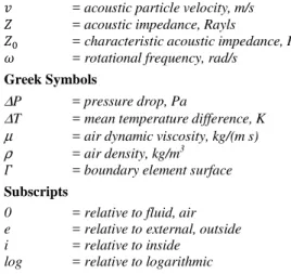
Model validation
The boundary element model described in the previous section was validated in terms of complex reflection coefficient for both situations including the unflanged case and the pipe terminated by an infinite flange. The validation was conducted by comparing the numerical results with the exact analytical solutions for an unflanged pipe (Levine and Schwinger, 1948) and for a pipe terminated by an infinite flange (Nomura et al., 1960). The comparison between the numerical and the exact analytical solutions for both the magnitude of
the reflection coefficient || and the dimensionless end correction /
are presented in Figs. 3(a) and 3(b), respectively.
Figure 3(a)
Figure 3(b)
Figure 3. Comparison between numerical and exact analytical solutions for an unflanged pipe and a pipe terminated by an infinite flange: (a) Magnitude of the reflection coefficient; and (b) dimensionless end correction.
The results depicted in both Figs. 3(a) and 3(b) show that a very good agreement between numerical results and theory can be achieved when the mesh refinement of the model is greater than forty elements per wavelength. Nevertheless, a slight discrepancy of ~0.2% is observed in the dimensionless end correction (Fig. 3(b)) at high frequencies, namely for > 2.5. This discrepancy is attributed to a non-sufficient mesh refinement, particularly at the open end region. For lower Helmholtz regions, as well as for the entire range of Helmholtz numbers in Fig. 3(a), the discrepancy is negligible.
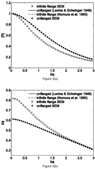
Results
Figure 4(a)
Figure 4(b)
Figure 4. Reflection coefficient as a function of / and : (a) magnitude of the reflection coefficient; and (b) dimensionless end correction.
Interestingly, the results illustrated in Fig. 4(a) show that, for pipes terminated by finite circular flanges, the behavior of
|| for a given 0 is not monotonic along / . This implies that, for certain values of 0, the corresponding magnitude of the reflection coefficient || may not lie between the curves representing the two extreme cases, as shown in Fig. 3(a).
The same non-monotonic behavior along / is observed for the dimensionless end correction / depicted in Fig. 4(b). This behavior becomes more evident when / is plotted against the ratio between pipe and flange radii / , as shown in Fig. 5.
The same figure shows that the numerical results for 0 are in very good agreement with the fit formula proposed by Dalmont et al. (2001) for the low frequency limit. Another interesting feature of Fig. 5 is that it shows that the non-monotonic behavior of / does not only appear along the / axis, but also along . This behavior seems to be critical in the region / ~ 0.4. This essentially means that, for a finite-flanged pipe with / ~ 0.4, the length correction / may significantly increase as → 0.8.
Figure 5. Dimensionless end correction as function of the ratio between pipe and flange radii / for different values of .
The numerical results presented in terms of surfaces (Figs. 4(a) and 4(b)) were used to derive approximate formulae for both || and
/ based on a least square polynomial fit scheme that minimizes the error e by
∗
, 8
where is the i-th element of an input vector , having an arbitrary integer number of elements , being 1. ∗ is the i-th element of a vector given by the polynomial ∗, whose coefficients are found in order to minimize the error . The resulting polynomial ∗ is approximated from the input vectors of || and / obtained numerically as functions of the Helmholtz number and the ratio between duct and flange radii / , and is given by
∗, /
, / ,
9
where the coefficients , are given for both || and / in Table 1 for the range of 0 3.0 and 0 / 1.
Naturally, the choice of the polynomial order in Eq. (9) will determine the goodness of the fit for the approximate formula. On the other hand, increasing the polynomial order implies in a higher number of polynomial coefficients, which may restrict the applicability of the fit formula. Thus, a tradeoff was established so as to provide simplicity of the fit formula and a reasonable goodness of fit. The result was a polynomial
∗
of order 10 (Eq. (9)), resulting on twenty one coefficients presented on Table 1.
Figure 6(a)
Figure 6(b)
Figure 6(c)
Figure 6(d)
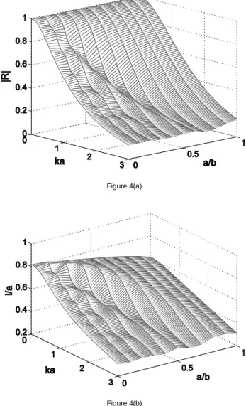
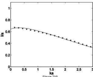
Figure 6. Comparison between approximate formula and numerical results for ||. (—) Approximate formula; (* * *) numerical results. The results are obtained for four different values of /: (a) 0.2; (b) 0.4; (c) 0.6; and (d) 0.8.
Replacing the coefficients from Table1 in Eq. (9) will lead to the fit formulas for both the magnitude of the reflection coefficient || and the end correction . Figures 6 and 7 present comparisons between numerical data and the values obtained by the fit formula (Eq. (9)) with the coefficients provided in Table 1. The results depicted in Figure 6 show a good agreement between fit formula and numerical data for the magnitude of the reflection coefficient
||. The maximum deviation from the numerical results is found at / = 0.4 and ~1, and corresponds to 4% (Fig. 7(b)).
Figure 7 shows the numerical and fit formula results for the dimensionless end correction l. Similarly to |R|, the maximum deviation between numerical and fit results is observed at a/b = 0.4 and ka = 0.7, corresponding to 2%. The deviations in both |R| and l are attributed to the inability of the polynomial to capture the non-monotonic behavior of these curves, particularly for / = 0.4.
As previously discussed, the deviations could be minimized by increasing the order of the polynomial (Eq. (9)).
However, increasing the accuracy of the fit formula by 1% would require an increase of the polynomial order by eight. That would imply in a significant increase of the number of coefficients, which in turn compromises the simplicity of the fit formula.
Conclusions
This paper investigates the behavior of the magnitude of the reflection coefficient || and the dimensionless end correction / at the open end of cylindrical pipes terminated by finite circular flanges in the absence of a mean flow. Moreover, the paper presented an approximate formula for both || and / based on a polynomial fit. The results from a numerical model of a pipe based on the boundary elements method have shown that || and / have a non-monotonic behavior in the regions between 0 ≤ / ≤ 1
and 0 ≤ ≤ 3.0. In the case of ||, the non-monotonic behavior is more significant at high frequencies, namely > 2 and within
0.2 ≤ / ≤ 0.5.
formulae for || and l/a were derived by a polynomial fit of the numerical results.
The fit formula agrees well with the numerical results, provided that 0 ≤ ≤ 3.0 and 0 ≤ /≤ 1. In the case of the magnitude of the reflection coefficient, the maximum deviation from the numerical results is equal to 4% at / = 0.4 and ~1. Similarly, in the case of / the maximum deviation from the numerical results is found at / = 0.4, corresponding to 2% at ~0.4.
Figure 7(a)
Figure 7(b)
Figure 7(c)
Figure 7(d)
Figure 7. Comparison between approximate formula and numerical results for /. (—) Approximate formula; (* * *) numerical results. The results are obtained for four different values of /: (a) 0.2; (b) 0.4; (c) 0.6; and (d) 0.8.
Acknowledgements
The authors would like to thank Dr. Gary Scavone for sharing the computational facilities from CAML, McGill University. Authors 1 and 2 would like to thank CNPq for supporting their research. All authors are thankful for the helpful suggestions provided by the reviewers of this paper.
References
Allam, S. and Abom, M., 2006, “Investigation of damping and radiation using full plane wave decomposition in ducts”, Journal of Sound and Vibration, 292, pp. 519-534.
Ando, Y., 1969, “On the sound radiation from semi-infinite circular pipe of certain wall thickness”, Acustica, 22, pp. 219-225.
Causs´e, R., Kergomard, J., and Lurton, X., 1984, “Input impedances of brass instruments - comparison between experiment and numerical models”,
J. Acoust. Soc. Am., 74, pp. 241-254.
Chandler, S. and Langdon, S., 1991, “Boundary Element Methods in Acoustics”, Computational Mechanics Publications, Boston.
Da Silva, A.R., 2008, “Numerical studies of aeroacoustic aspects of wind instruments”, Ph.D. thesis, McGill University.
Dalmont, J.P., Nederveen, C.J., and Joly, N., 2001, “Radiation impedance of tubes with different flanges: Numerical and experimental investigations”, Journal of Sound and Vibration, 244, pp. 505-534.
Fahy, F. and Walker, J., 2004, “Advanced Applications in Acoustics, Noise and Vibration”, Spoon Press, London.
Levine, H. and Schwinger, J., 1948, “On the radiation of sound from an unflanged circular pipe”, Physical Review, 73, pp. 383-406.
Munt, R.M., 1990, “Acoustic transmission properties of a jet pipe with subsonic jet flow: I. the cold jet reflection coefficient”, Journal of Sound and Vibration, 142, pp. 413-436.
Nomura, Y., Yamamura, I., and Inawashiro, S., 1960, “On the acoustic radiation from a flanged circular pipe”, Journal of the Physical Society of Japan, 15, pp. 510-517.
Norris, A.N. and Sheng, I.C., 1989, “Acoustic radiation from a circular pipe with an infinite flange”, Journal of Sound and Vibration, 135, pp. 85-93.
Selamet, A., Ji, Z.L., and Kach, R.A., 2001, “Wave reflections from duct terminations”, J. Acoust. Soc. Am., 109.
Silva, A.R. d., Scavone, G.P., and Lefebvre, A., 2009a, “Sound reflection at the open end of axi symmetric ducts issuing a subsonic mean flow: A numerical study”, Journal of Sound and Vibration, 327, pp. 507-528.