ORIGINAL ARTICLE
Improved tree height estimation of secondary forests
in the Brazilian Amazon
Henrique Luis Godinho CASSOL1,*, Yosio Edemir SHIMABUKURO 1, João Manuel de Brito CARREIRAS 2,
Elisabete Caria MORAES 1
1 Instituto Nacional de Pesquisas Espaciais - INPE, Divisão de Sensoriamento Remoto, São José dos Campos, SP, Brasil 2 University of Sheffield, National Centre for Earth Observation (NCEO), Sheffield, UK
* Corresponding author: [email protected]
ABSTRACT
This paper presents a novel approach for estimating the height of individual trees in secondary forests at two study sites: Manaus (central Amazon) and Santarém (eastern Amazon) in the Brazilian Amazon region. The approach consists of adjusting tree height-diameter at breast height (H:DBH) models in each study site by ecological species groups: pioneers, early secondary, and late secondary. Overall, the DBH and corresponding height (H) of 1,178 individual trees were measured during two field campaigns: August 2014 in Manaus and September 2015 in Santarém. We tested the five most commonly used log-linear and nonlinear H:DBH models, as determined by the available literature. The hyperbolic model: H = a.DBH/(b+DBH) was found to present the best fit when evaluated using validation data. Significant differences in the fitted parameters were found between pioneer and secondary species from Manaus and Santarém by F-test, meaning that site-specific and also ecological-group H:DBH models should be used to more accurately predict H as a function of DBH. This novel approach provides specific equations to estimate height of secondary forest trees for particular sites and ecological species groups. The presented set of equations will allow better biomass and carbon stock estimates in secondary forests of the Brazilian Amazon.
KEYWORDS: tree height-diameter (H:DBH) model; nested model; indicative variable; height growth; ecological species groups
Estimativa melhorada de altura de árvores em florestas secundárias da
Amazônia brasileira
RESUMO
Este trabalho apresenta uma nova abordagem para a estimativa de altura de árvores em florestas secundárias em duas áreas de estudo na Amazônia brasileira: Manaus (Amazônia central) e Santarém (Amazônia oriental). A abordagem consistiu em ajustar modelos hipsométricos separados por área de estudo e grupos ecológicos de espécies: pioneiras, secundárias iniciais e secundárias tardias. No total, 1178 árvores foram medidas em diâmetro e altura em duas etapas de campo: agosto de 2014 em Manaus e Setembro de 2015 em Santarém. Foram testados cinco modelos log-lineares e não lineares mais utilizados na literatura. O modelo hiperbólico: H = a.D/(b+D) foi o que apresentou o melhor ajuste quando avaliado com os dados de validação. Diferenças significativas nos parâmetros de ajuste foram observadas entre as espécies pioneiras e secundárias de Manaus e Santarém pelo teste F, significando que equações específicas por grupos ecológicos e área de estudo deveriam ser utilizadas para estimar a altura (H) a partir do diâmetro (D) com maior acurácia. Esta nova abordagem fornece equações específicas para localidade e grupo ecológico, para estimar a altura das árvores em florestas secundárias. O conjunto de equações desenvolvidas permitirá melhorar as estimativas de biomassa e a quantificação dos estoques de carbono nas florestas secundárias da Amazônia brasileira.
PALAVRAS-CHAVE: modelos hipsométricos; modelos aninhados; variável indicadora; taxa de crescimento em altura; grupos
ecológicos de espécies
INTRODUCTION
In the Amazon region, height-diameter at breast height (H:DBH) models are important because dense forest understory makes it difficult and time-consuming to view the top of the canopy to measure the tree heights. Several H:DBH models have been proposed for old-growth tropical forests for that purpose (Feldpausch et al. 2011; 2012; Hunter
et al. 2013), however, they are scarce for secondary forests (Lucas et al. 2002; Neeff and Santos 2005). For instance, Lucas et al. (2002) used genus-specific nonlinear models to estimate tree height based on diameter for the most common species from a secondary forest in Manaus (central Amazon). Conversely, Neeff and Santos (2005) estimated tree height, and its increments, at stand-level age based on the Bertalanffy– Chapman–Richards model in a secondary forest in Santarém (eastern Amazon). Other models related to H:DBH include the logistic, Weibull, and Richards models (Fang and Bailey 1998; Huang et al. 2000).
The choice of the best model, however, depends on the relation between tree height and DBH, which, in turn, can be associated with physical and biological factors at tree- and stand-level (Poorter and Bongers 2006; Weiskittel et al. 2011). At tree level, H:DBH scaling may be represented by the stem-form factor, which can be indicative of the tree’s position within the forest stand (Weiskittel et al. 2011). The stem-form factor is defined as the ratio of the volume of a tree, or its part, to the volume of a cylinder with the same size (height) and cross section (DBH). Therefore, the tree may present a conical or cylindrical shape depending on its stem-form factor. For example, dominant trees often have a DBH greater than 30 cm, enjoy favorable light conditions, and have cylindrical shapes (Assmann 1970). In these trees, the scaling exponent between H and DBH is equal or similar to two-thirds, and the allometry assumes an elastic similarity model (Norberg 1988). Meanwhile, most sub-dominant and pioneer species follow a geometric similarity model (H:DBH scaling = 1.0), i.e., the trunk diameter will scale in direct proportion to the tree height (Sposito and Santos 2001). However, when H:DBH scaling ~2.0 there is a constant stress model, which is commonly caused by wind or other stresses (Sposito and Santos 2001).
At stand level, tree growth depends on forest structure, dominance type, tree density, species composition, and site environmental conditions (Weiskittel et al. 2011). Therefore, tree growth rate and H:DBH scaling are influenced by environmental conditions and functional traits at both tree and stand levels (Selaya et al. 2008; Chazdon 2014). Sites with nutrient-rich soils and favorable climate conditions promote fast tree growth; pioneer species seek these resources in order to quickly colonize newly deforested areas (Chazdon 2014). The tree-height growth is highest at sites with better quality of environmental conditions, even though the maximum increase could be reached at the same age in poor sites (Weiskittel et al.
2011). Several studies have been carried out to develop site-based H:DBH models exploring these different environmental conditions in varying forest types (Pillsbury et al. 1995; Huang
et al. 2000; Feldpausch et al. 2011). Huang et al. (2000) noted that the application of H:DBH models from one region to another may result in an average bias of 29%.
Different species make use of distinct strategies to reach sunlight, promoting fast or slow growth, depending on resource availability and plant physiology (Poorter et al.
2012). In Amazonian secondary forests dominated by Cecropia
sp. and Vismia sp., the pioneer species showed fast growth and aboveground biomass (AGB) accumulation, reaching 110–115 Mg ha-1 during the first 10–15 years (Lucas et al.
2002). As a strategy, these pioneer species intercept more light per unit leaf mass to support their fast growth than late successional species, contributing to the efficient conversion of mass to height (Selaya et al. 2008). To maintain rapid growth, pioneer species also present high leaf turnover in the upper-canopy, forming a monolayer leaf arrangement that covers bare soil. In contrast, these species need to form slender stems with low wood density to support such accelerated tree growth, which inevitably reduces their life span (Poorter and Bongers 2006; Selaya et al. 2008).
Late successional tree species are characterized by lower growth rates, resulting in the requirement for greater wood densities to support larger canopies and to reduce the risk of hollow stem formation (Poorter and Bongers 2006). These species are generally taller and long-lived when compared to pioneer species, although the photosynthetic rate by leaf mass is smaller (Chazdon 2014). Therefore, carbon assimilation by long-lived late successional species is lower and more persistent compared with short-lived pioneer species (Santiago et al.
2004). Such differences in vertical growth among species have significant implications for AGB accumulation in tropical forests (Feldpausch et al. 2011; Feldpausch et al. 2012). Tree height is highly variable in the Amazon forest, therefore it is important that this parameter is included in equations to estimate tree AGB more accurately (Lefsky et al. 2010; Chave et al. 2014; Sawada et al. 2015). Feldpausch et al. (2011) observed a tree height gradient from northeast to southwest Amazon, with the tallest trees in the Guiana Shield and the shortest in the southern Amazon. By including tree height in the AGB models, biomass estimates errors were consistently reduced from 66 to 48 Mg ha-1 from the eastern-central to the western Amazon,
respectively (Feldpausch et al. 2012). Furthermore, the AGB of the Brazilian Amazon is often estimated by applying allometric equations generated from only primary or old-growth forest species, which may lead to overestimation (by 10–60%) when applied for AGB secondary forest trees (Nelson et al. 1999).
also expected to find significant differences between groups of ecological species across the study sites owing to different environmental and climate conditions. It has been reported that maximum tree heights at stand level vary among primary forests across the Amazon (Feldpausch et al. 2011, 2012; Lefsky
et al. 2010); however, it is unclear whether these differences also occur over secondary forests. For this investigation, we evaluated five commonly used H:DBH models adjusted to different ecological species groups occurring in two sites, with the aim of improving tree height estimation in secondary forests in the Brazilian Amazon.
MATERIAL AND METHODS
Study area and data
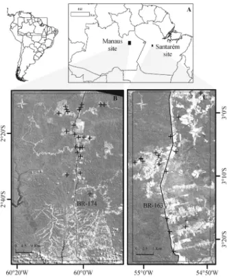
This study was carried out at two sites in the Brazilian Amazon: Manaus (Amazonas State) in the central Amazon region, and Santarém (Pará State) in the eastern Amazon region. At the Manaus site, the sampling plots were chosen on either side of the BR-174 highway, 70 km to the north of the city of Manaus. At the Santarém site, the sampling plots were chosen close to the Tapajós National Forest (FLONA Tapajós) on either side of the BR-163 highway, 100 km to the south of the city of Santarém (Figure 1).
According to Chave et al. (2005), both study sites are classified as ‘moist forest’, with less than 5 months averaging < 100 mm month-1 of rainfall during the dry season. The
dry season length is shorter in Manaus (3.1 months) than in Santarém (4.5 months) (Malhi et al. 2004). Manaus receives an average annual rainfall of 2,200 mm, which is slightly higher than that received at Santarém (2,000 mm) (Asner
et al. 2003). The mean annual temperature at both sites is approximately 26 °C. Soils are predominantly nutrient-poor clay oxisols with some sandy ultisols (Silver et al. 2000).
Secondary forests in Manaus and Santarém occur in a region dominated by terra firme old-growth dense forests, which have a similar average canopy height (26 and 28 m, respectively), but very different height distributions (Hunter et al. 2015). Santarém primary forests present a bi-modal distribution of tree-canopy heights, one comprised of emergent trees (average 35–40 m heights) and the other comprised of sub-dominant trees (average 15–30 m), while Manaus primary forests show a near unimodal Gaussian distribution, with an average 26 m canopy height (Hunter et al. 2015). Additionally, open tropical forests occur in the east side of FLONA Tapajos, with these being widely dominated by palm trees such as babaçú (Attalea speciosa Mart.) and inajá
(A. maripa (Aubl.) Mart.) on sandy soils (Prates-Clark et al.
2009; personal observation).
In both study sites, only advanced secondary forests (age > 16 years) were measured in a 60 × 100 m nested plot. All sampling plots were randomly selected based on the age of the secondary forest and on land-use history (period of active land use and frequency of land clearance), assessed through the analysis of extensive Landsat sensor time-series data (Carreiras
et al. 2014). Field measurements were conducted during August 2014 in Manaus (23 plots) and September 2015 in Santarém (16 plots) (Figure 1) as part of the REGROWTH-BR project (Carreiras et al. 2014).
All trees with a DBH (at 1.3 m height) greater than or equal to 5 cm were measured within a 10 × 100 m plot. Trees with a DBH ≥ 10 cm were measured within a 20 × 100 m plot, and trees with a DBH ≥ 20 cm were measured within a 60 × 100 m plot. All trees were identified botanically to species level or marked as unknown (three cases; see Supplementary Material, Table S1).
Trees were randomly selected and heights were measured at each nested plot (circa 25 measurements per plot) with a laser hypsometer (True Pulse 200TM, LaserInc Technology, Denver,
CO, USA), whereas DBH was measured with a girth tape. All trees with broken or damaged crowns, and all palms, were excluded from the analysis.
The individuals were assigned to an ecological species group (ESG): pioneers (P), early secondary stage (ES), or late secondary stage (LS). This was based on the information collected from the literature and from the Global Wood Density Database (Zanne et al. 2009, see Supplementary
Material, Table S1). The formal Mann-Whitney U test was used to compare differences between wood densities among the three ESGs. The Bonferroni correction for pair-wise Mann-Whitney U test alpha was α/3 = ~0.0167. Therefore, we used median wood density thresholds to assign a species to a specific ESG when the previous classification was not found in the literature, e.g., pioneers ≤ 0.5 g cm-3, 0.5 g cm-3 < early secondary ≤ 0.59 g cm-3,
and late secondary < 0.74 g cm-3.
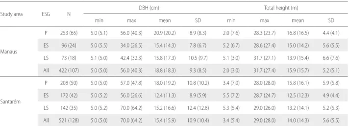
Height and DBH data from 1,178 individual trees ranging from 5-70 cm in diameter, corresponding to 188 species and 52 families, were collected during the field campaign: 529 individuals in Manaus and 649 in Santarém. Before adjusting H:DBH models, the data were stratified by ecological species and study site, and then split into two subsets: the training subset (80%) for model fitting, and the remainder (testing subset) for model validation (Table 1). The H:DBH ratio was evaluated by study site using the Mann-Whitney U test to support a priori
any difference in tree architecture (Feldpausch et al. 2011). The Mann-Whitney U test was performed using the R statistical program (R Development Core Team 2008).
Model selection and comparison of fitted models
Several linear and nonlinear allometric models have been proposed to describe the relationship between tree height and diameter (Fang and Bailey 1998; Huang et al. 2000). In this study, we tested five widely used H:DBH models (Fang and Bailey 1998; Huang et al. 2000; Feldpausch et al. 2011) (Table 2). Only H:DBH models with up to three parameters were selected in order to avoid problems with over-parameterization in nonlinear regression estimation, as reported by Fang and Bailey (1998).
To select the most suitable model, we compared the ability of these five allometric models to predict tree height at each ESG by study site. The nonlinear least squares (nls) command from R was used to estimate the parameters in all nonlinear models (Bates and Watts 1990), and the ordinary least squares (lm) command in the case of the log-linear model (m1).
The following statistics were used to select the best models in terms of goodness-of-fit using the training subset (Motulsky and Christopoulos 2003): (i) absolute and relative root mean square error (RMSE); and (ii) Akaike information criterion (AIC) weights (Wagenmakers and Farrel 2004). The relationship between standardized residuals and predicted height was evaluated visually through scatterplots in each model to account for heteroskedasticity. Additionally, a formal Breusch-Pagan test against heteroskedasticity (Neter et al. 1996) was performed using the lmtest package in R.
Model validation and presence of outliers
Prediction bias was calculated by subtracting the predicted height from the observed height (measured) using the testing subset. A null hypothesis, whereby the bias is equal to zero, was tested by
t-test, with α = 0.05 significance level. Therefore, the root mean square error of prediction (RMSEP) was calculated by Eq. (1) (Hastie et al. 2009): RMSEP = (bias² + variance)1/2. The first
term in Eq. (1) is relative to the average prediction bias and the second term refers to the variance-bias, which in turn, is related to the spread of points around the mean prediction.
The presence of outliers was evaluated in both training and testing subsets using outlier in the “outliers” package of R program. The presence of outliers was verified by observing the spread of the residuals. If confirmed, the model selection and validation were iteratively repeated to improve model fitting. This process was performed twice with removal of 19 outliers from the analysis, including the training and testing subsets.
We arbitrary attributed a descending rank order to choose only one model based on highest AIC weight: value 5 for the best model (highest), and 1, for the worst (lowest). The best ranked fitted model (sum of rank values) was then used to analyze differences between ESG and study sites using an indicator regression approach.
Table 1. Summary of the training and validation datasets (in parentheses) by study area and ecological species groups (ESG). N = number of trees, min = minimum, max = maximum, SD = standard deviation, DBH = diameter at breast height, P – pioneers, ES – early secondary, LS – late secondary.
Study area ESG N
DBH (cm) Total height (m)
min max mean SD min max mean SD
Manaus
P 253 (65) 5.0 (5.1) 56.0 (40.3) 20.9 (20.2) 8.9 (8.3) 2.0 (7.6) 28.3 (23.7) 16.8 (16.5) 4.4 (4.1)
ES 96 (24) 5.0 (5.5) 34.0 (26.5) 15.4 (14.3) 7.8 (6.7) 5.2 (6.7) 28.6 (27.4) 15.0 (14.2) 5.6 (5.5)
LS 73 (18) 5.1 (5.0) 42.4 (32.3) 15.8 (17.3) 10.5 (9.7) 5.1 (3.0) 31.7 (27.1) 13.9 (15.4) 6.6 (7.6)
All 422 (107) 5.0 (5.0) 56.0 (40.3) 18.8 (18.3) 9.3 (8.5) 2.0 (3.0) 31.7 (27.4) 15.9 (15.7) 5.2 (5.1)
Santarém
P 208 (50) 5.0 (5.0) 57.0 (47.8) 18.0 (19.2) 10.8 (10.2) 3.4 (7.0) 28.0 (28.0) 15.8 (16.1) 5.9 (5.8)
ES 172 (42) 5.0 (5.2) 56.0 (26.6) 12.4 (11.3) 8.9 (5.9) 5.5 (7.2) 28.7 (24.7) 12.5 (12.3) 4.9 (4.4)
LS 142 (35) 5.0 (5.2) 70.0 (64.2) 15.2 (16.6) 12.4 (12.8) 5.3 (5.4) 29.0 (26.0) 13.2 (14.1) 5.2 (5.3)
Comparison of H:DBH models by ecological species group and study site
The indicator regression approach was used to evaluate full and reduced nested models with a simple ANOVA F-test (Bates and Watts 1990; Neter et al. 1996). The indicator variable, or dummy variable, is an artificial variable created to represent an attribute with two or more distinct categories/levels, which, in our case, was represented by a study site or a specific ESG (Neter et al. 1996).
In the full model, the indicator variable could only take the values 0 and 1, corresponding to each study site or ESG, and the reduced model was fitted using the whole dataset without the indicator variable. However, to avoid over-parametrization of the full models, the ANOVA F-test was performed to compare each pair of ESGs per study site, because the difference in parameter estimation may be caused by only two or more indicator variables involved in the analysis, and this method reduces the number of parameters whilst retaining validation of the nested approach (Huang et al. 2000).
For instance, if the response function was modeled by the log-linear model between pioneers and early secondary forest species, the full-model of H:DBH would have three parameters (Neter et al. 1996) [Eq. (2): h = a+b log (DBH)+cG1 log (DBH)+ ε; where
a and b are log-linear parameters, c represents the parameters related to indicator variable, and ε is the regression error; G1 refers to the indicator variable of a specific ESG (pioneer or early secondary)]. In this case, the reduced model has only two parameters (a and b). Considering that the response function (2) is for pioneers for which G1 = 0, then the model would take the form: h=a+b log(DBH). If the response function is for early secondary species for which G1 = 1, then Eq. (2) would take the form: h = a+b log(DBH)+cG2 log(DBH), and so on. Similarly, the analysis can be performed with all nonlinear models described in Table 1, and with all other ESG pairs or study sites.
The equality of the two models was tested by considering the null hypothesis, H0, whereby indicator parameters in the full model are equal to zero, against the alternative hypothesis,
H1, whereby at least one parameter differs from zero using the F-test according to Motulsky and Christopoulos (2003). ANOVA F-test was performed in R (R Core Team 2008) with a 0.95 confidence level.
Finally, we estimated the relative growth height rate (HGR) by taking the derivative of the selected model by its diameter. The fitted curves for relationships between HGR and H:DBH were provided.
RESULTS
Ecological species groups
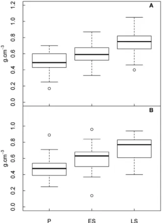
Median differences in wood density between ESG pairs differed from zero (Mann-Whitney U test: W = 64, p < 0.016), suggesting that wood density values could be used to separate species groups. Then, we used median wood density to assign species into an ESG when these were not available in the literature (in this case 22 of 323 species collected, Supplementary Material, Table S1).
Wood density outliers, marked with an open circle in Figure 2, indicate the low wood density of Hevea brasiliensis
(Willd. ex A. Juss.) Müll.Arg. (0.40 g cm-3, late secondary
species) in Manaus. In Santarém, outliers were represented by high wood density of Neea oppositifolia Ruiz & Pav. (0.89 g cm-3, pioneer species) and Sloanea nitida G. Don. (0.96 g cm-3,
early secondary species), and low wood density of Jacaratia spinosa (Aubl.) A.DC. (0.14 g cm-3, early secondary species).
Table 2. Height-diameter models selected for analysis. H = total height (m); DBH = diameter at breast height (1.3 m above ground).
Model number Model form Model type
m1 H = a + b.log.DBH Log-Linear
m2 log H = a + b.log.DBH Log-Log
m3 H = a.DBH/(b+DBH) Hyperbolic
m4 H = a.(1 - c.exp(-b.DBH)) Monomolecular m5 H = a.(1 - exp(b.DBH)c) Chapman-Richards
The simple ratio H:DBH of the secondary forest trees was significantly different between study sites, as determined by the Mann-Whitney U test: W = 133246, p < 0.001 (Manaus = 0.9037; Santarém = 1.0588). Tree diameters from secondary forests in Manaus (median 19.8 cm) were significantly different from those in Santarém (median 12.2 cm), and the same was observed for tree heights in Manaus (median 16.7 m) and Santarém (median 12.8 m), p < 0.001. This indicates that the H:DBH relationship followed a different distribution at each study site, considering that forests at both study sites are of similar average age (circa 23 years after clear cut).
Models’ goodness-of-fit
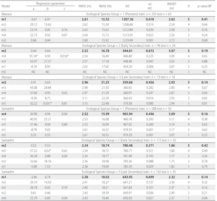
Two-parameter models showed the best goodness-of-fit given by the sum ranked order of the lowest AIC (Table 3): hyperbolic model (sum of 21 points) and log-log model (19 points). The monomolecular model (18 points) also had a low AIC among the three-parameter models. All regression parameters were significant at α = 0.05 for all models, with the exception of the Weibull model for early secondary species in Manaus, the Chapman-Richards model for early secondary species in Santarém, and for late secondary species in Manaus (Table 3).
Table 3. Fitting statistics of the tested H:DBH models by ecological species groups and study area. RMSE and RMSE are the absolute and relative root mean square error, respectively. RMSEP is the RMSE of prediction. R is the value of the rank order based on the lowest wiAIC (in bold). wiAIC – weights of Akaike information criterion; BP - Breusch-Pagan test. *Non-significant parameters for alpha = 0.05. NC – do not converge.
Model Regression parameter RMSE (m) RMSE (%) AIC wi
AIC
RMSEP
(m) R p-value BP
a b c
Manaus Ecological Species Group = 1 (Pioneers) train. n = 255 test n = 63
m1 -3.67 6.97 2.61 15.55 1207.36 0.618 2.62 5 0.41
m3 29.12 13.65 2.62 15.58 1208.68 0.319 2.59 4 0.64
m5 23.74 0.05 0.76 2.63 15.62 1212.89 0.039 2.58 3 0.76
m4 22.73 0.92 0.07 2.64 15.72 1213.95 0.023 2.56 2 0.24
m2 0.66 0.44 2.68 15.92 1219.99 0.001 2.73 1 0.68
Manaus Ecological Species Group = 2 (Early Secondary) train. n = 96 test n = 24
m2 0.44 0.64 2.52 16.78 444.61 0.672 3.07 5 0.19
m4 55.16* 0.93 0.016* 2.54 16.89 446.80 0.225 3.09 4 0.65
m3 43.97 27.21 2.57 17.18 448.48 0.097 3.03 3 0.88
m1 -8.18 8.95 2.65 17.65 454.20 0.006 3.07 2 0.25
m5 NC NC NC NC NC NC NC 1 NC
Manaus Ecological Species Group = 3 (Late Secondary) train. n = 73 test n = 18
m2 0.41 0.63 2.96 21.25 359.68 0.456 2.93 5 0.14
m3 43.08 28.84 2.98 21.50 360.65 0.282 2.80 4 0.07
m4 37.60 0.93 0.03 2.97 21.29 360.91 0.247 2.87 3 0.04
m1 -8.30 8.75 3.11 22.29 366.43 0.016 2.95 2 0.05
m5 32.22 0.031* 0.81 3.15 22.48 379.58 0.000 2.94 1 0.01
Santarém Ecological Species Group = 1 (Pioneers) train. n = 208 test n = 50
m4 30.90 0.94 0.04 2.52 15.99 965.94 0.446 3.09 5 0.16
m3 40.95 25.21 2.53 16.08 966.78 0.293 3.11 4 0.38
m5 31.46 0.04 0.84 2.53 16.04 967.02 0.260 3.14 3 0.63
m1 -8.78 9.02 2.61 16.52 978.35 0.001 3.17 2 0.62
m2 0.53 0.55 2.61 16.52 979.29 0.001 3.07 1 0.25
Santarém Ecological Species Group = 2 (Early Secondary) train. n = 172 test n = 42
m2 0.53 0.53 2.34 18.74 780.48 0.371 1.86 5 0.42
m5 37.22 0.02* 0.62 2.34 18.72 780.77 0.321 1.80 4 0.49
m4 30.28 0.88 0.04 2.34 18.77 781.80 0.192 1.77 3 0.26
m3 33.66 18.16 2.36 18.98 783.36 0.088 1.75 2 0.78
m1 -5.08 7.53 2.38 19.04 785.59 0.029 1.83 1 0.79
Santarém Ecological Species Group = 3 (Late Secondary) train. n = 142 test n = 35
m1 -3.46 6.74 2.38 18.03 643.95 0.699 2.32 5 0.14
m3 29.19 14.50 2.41 18.27 647.21 0.137 2.30 4 0.32
m5 28.78 0.02 0.59 2.40 18.21 647.83 0.101 2.37 3 0.16
m2 0.61 0.46 2.43 18.39 649.91 0.036 2.49 2 0.21
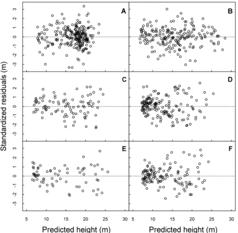
Figure 3. Plots of standardized residuals against predicted height using nonlinear least squares fitting of the hyperbolic model for pioneer (A), early secondary (C), and late secondary (E) species in Manaus and Santarém (B, D, and F), respectively.
The visualization of standardized residuals against predicted height showed the absence of heteroskedasticity (Figure 3), which further supports the non-significant results of the Breusch-Pagan test (Table 3). The residuals were drawn only for the selected hyperbolic model.
Based on the ranked model (Table 3), the hyperbolic model (m3) presented satisfactory results for all ESGs without being the best for a specific ESG. The prediction error of the hyperbolic model extended from RMSEP = 1.75 to 3.11 m (Table 3). Considering that bias is close to zero by the null hypothesis, we did not reject H0 in any of the ESG cases, meaning that the average bias was equal to zero with dfF (n-1) degrees of freedom. Because the mean bias was not significantly different from zero in all models fitted by a one sample t-test (p > 0.05), variance of prediction was a large source of error. In general, the hyperbolic model performed well, although it overestimated tree height above 20 m, independent of age, as this seems to be the height at which this model begins to consistently underestimate values (Figure 4).
Comparison of H-DBH models by study site and ESG
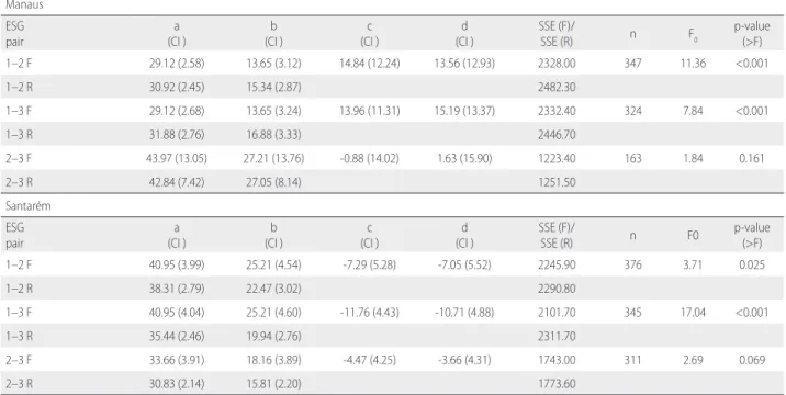
The null hypothesis was not rejected for the ESG 2–3 pair (early secondary and late secondary species) at both study sites (Table
4), suggesting that parameters c and d from the full models were different from zero in these cases (p > 0.05). Based on the results of the paired F-test, and the estimated parameters of the full model, we concluded that secondary species (early and late) had a similar H:DBH relationship in both study sites, hereafter grouped into one class, while pioneer species belonged to another class.
Table 4. Fitted parameters of the full (F) and reduced (R) hyperbolic model by ESG pairs. CI = 95% confidence interval, as shown in parentheses. SSE (F) and SSE (R) are the sum of square error for full and reduced models, respectively. a, b, c, and d are the parameters. ESG-Pair (ecological species group pairs): 1–2 (pioneers-early secondary species), 1–3 (pioneers-late secondary species), 2–3 (early-late secondary species).
Manaus ESG pair
a (CI )
b (CI )
c (CI )
d (CI )
SSE (F)/
SSE (R) n F0
p-value (>F) 1–2 F 29.12 (2.58) 13.65 (3.12) 14.84 (12.24) 13.56 (12.93) 2328.00 347 11.36 <0.001
1–2 R 30.92 (2.45) 15.34 (2.87) 2482.30
1–3 F 29.12 (2.68) 13.65 (3.24) 13.96 (11.31) 15.19 (13.37) 2332.40 324 7.84 <0.001
1–3 R 31.88 (2.76) 16.88 (3.33) 2446.70
2–3 F 43.97 (13.05) 27.21 (13.76) -0.88 (14.02) 1.63 (15.90) 1223.40 163 1.84 0.161
2–3 R 42.84 (7.42) 27.05 (8.14) 1251.50
Santarém ESG pair
a (CI )
b (CI )
c (CI )
d (CI )
SSE (F)/
SSE (R) n F0
p-value (>F) 1–2 F 40.95 (3.99) 25.21 (4.54) -7.29 (5.28) -7.05 (5.52) 2245.90 376 3.71 0.025
1–2 R 38.31 (2.79) 22.47 (3.02) 2290.80
1–3 F 40.95 (4.04) 25.21 (4.60) -11.76 (4.43) -10.71 (4.88) 2101.70 345 17.04 <0.001
1–3 R 35.44 (2.46) 19.94 (2.76) 2311.70
2–3 F 33.66 (3.91) 18.16 (3.89) -4.47 (4.25) -3.66 (4.31) 1743.00 311 2.69 0.069
2–3 R 30.83 (2.14) 15.81 (2.20) 1773.60
Height growth by site and species groups
The hyperbolic model was relatively easy to fit, achieved good validation results, and was meaningful in terms of the biological interpretation of its parameters. In this function, a
represents total height at maximum DBH (asymptote), and b
is the DBH when tree height reaches half the asymptote. Thus, a first derivative of the hyperbolic model allows us to obtain the absolute rate of height growth by DBH unit [Eq. (3): dy/ dx= ab/(b+x)²]. Therefore, when DBH approaches zero, a/b
represents the maximum height increment by DBH unit (m cm-1). Disregarding other underlying dynamic processes of
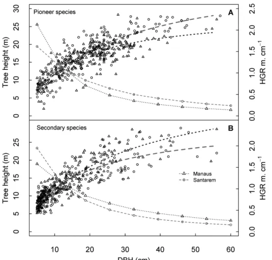
H:DBH relationships, we observed that pioneers in Manaus had the highest HGR. The HGR in pioneer species from Manaus was 2.13 m cm-¹, meaning that for every centimeter in diameter
increment, height increased more than 2 m. Santarém pioneers had a HGR = 1.62 m cm-¹ (Figure 5). Conversely, secondary
species in Santarém had a greater HGR than those in Manaus, HGR = 1.95 and 1.58 m cm-¹, respectively.
Table 5. Fitted parameters of full (F) and reduced (R) hyperbolic models by study area for pioneer and secondary species. CI = 95% confidence interval, as shown in parentheses. SSE (F) and SSE (R) are the sum of square error for full and reduced models, respectively. a, b, c, and d are the parameters.
Groups a
(CI )
b (CI )
c (CI )
d (CI )
SSE (F)/
SSE (R) n F0
p-value (>F)
Pioneers F 29.12 (2.54) 13.65 (3.08) 11.82 (4.72) 11.56 (5.42) 3020.80 458 19.105 p<0.001
Pioneers R 34.15 (2.40) 18.89 (2.83) 3275.00
Secondary F 42.84 (6.64) 27.05 (7.28) -12.01 (5.55) -11.24 (5.90) 3025.10 476 12.463 p<0.001
Secondary R 34.00 (2.19) 18.56 (2.30) 3184.80
Pioneer species had high initial HGR in Manaus compared with secondary species, and this decreased with increasing diameter. Compared with Manaus, pioneer species in Santarém showed a greater HGR for large trees (Figure 5). The increase in height growth fell below 0.20 m cm-1 at DBH > 40 cm. This
decline can be expected to continue until the regenerating forest becomes structurally similar to the average canopy heights of the mature forest, which is reported to be 26 m in Manaus and 28 m in Santarém (Hunter et al. 2015). Based on height modelling of secondary forests in Santarém, height initially increases by a maximum of 2 m per year, and then falls below 0.25 m per year at age 30 (Neeff and Santos 2005). Pioneer species in Manaus exhibited fast growth in the first years; this was around 30% higher than that observed in Santarém (Figure 5). However, later in life, they had about 50% smaller HGR than pioneers in Santarém (DBH = ~40 cm).
DISCUSSION
The hyperbolic model presented the best validation results among the most common models. We found statistical differences between pioneer and secondary species for H:DBH relationships, but not between early and late secondary species. These differences were consistent across sites, probably due to environmental and climate conditions. The HGR presented distinct behavior among ESGs and between sites.
Model selection for goodness-of-fit comparison
According to Fang and Bailey (1998), different H:DBH models with the same number of parameters usually result in similar goodness-of-fit when the nonlinear least square method is used on the same data set. Feldpausch et al.
(2011) observed that log-log models (two parameters) were the most suitable for estimating tree height in dry and wet forests, with no trend observed in their residuals by diameter class. Asymptotic functions with three parameters, such as the Weibull model, provided good estimates of ecologically meaningful H max in moist forests (Feldpausch
et al. 2011). Conversely, when one or two parameters are introduced in the model (e.g., three or four parameters instead of two), biological interpretation of parameters may be lost (Fang and Bailey 1998). Convergence could not be attained as easily as when using the Weibull and Chapman-Richards models (Table 3).
In this study, the hyperbolic model was found to produce the most satisfactory fit among the tested models, which was consistent with previous studies that also satisfactorily tested this model for adjusting H:DBH relationships (Fang and Bailey 1998; Huang et al. 2000). Nevertheless, due to the adjusted asymptote being close to 40 m for secondary forest trees, the hyperbolic model tended to underestimate the height of large trees, therefore its application in old growth forest should be avoided.
Separating H:DBH models by study site and ESG
Statistical differences were found between study sites in H:DBH relationships. Considering that the secondary forest plots were at a similar age (~23 years), the most important local factors influencing H:DBH relationships are the stand density, basal area, and species composition (Gómez-García et al.
2016). Basal area and stand density are the first parameters to reach similarity in mature forests (within 20–40 years), while similarity in species composition can take longer (Feldpausch
et al. 2005; Neeff and Santos 2005).
Owing to resource competition, trees of the same DBH usually have greater height in denser stands. We estimated average stand basal area as 22.3 and 23.7 m² ha-1 in secondary
forest plots in Santarém and Manaus, respectively, which may be indicative of greater average tree height in Manaus. Hunter
et al. (2013) reported a greater average basal area of primary forests in FLONA Tapajós (31 m² ha-1), with average canopy
height taller than that in Reserva Ducke, near Manaus site (28.7 m² ha-1). Such differences are probably due to primary
forests from Santarém having larger trees with DBH > 60 cm than Manaus primary forests (Vieira et al. 2005), increasing both the average basal area and the mean canopy height, which is not observed in secondary forests.
Some climatic variables, such as greater annual precipitation, shorter dry season length, and greater mean annual air temperature, could be drivers of greater relative tree growth in central Amazon secondary forests (Malhi et al. 2004). From a hydraulic perspective, it would be expected that, for a given DBH, trees would be shorter with increasing water deficit. Hence, the application of H:DBH models from the moderately seasonal central Amazon may overestimate tree height in the dry forest, and underestimate it in the wet regions (Malhi et al. 2004).
Regarding ESG-specific H:DBH models, pioneer and secondary species may be regarded as different groups at our study sites. Although pioneer species grow faster than late successional species (Selaya et al. 2008), we found a different behavior in pioneer species in Santarém. In this study site, pioneer species showed similar behavior to early secondary species, which can be supported by interpretation of the magnitude of the confidence intervals of the regression parameters in Table 4.
It is probable that pioneer species from Santarém are still competing for resources with other secondary trees, while in Manaus, short-lived species are being replaced by other long-lived secondary species. The most important pioneer species in Manaus, Vismia spp., Cecropia spp., and
Bellucia spp., are short-lived (20–30 years), and are virtually absent from old growth forest (Lucas et al. 2002). Secondary forests in Santarém are dominated almost exclusively by
Guatteria poeppigiana Mart., a pioneer species with a lifespan of 54 years (Holm et al. 2014). The high growth rate of large trees (DBH > 60 cm) of late secondary species may be a major cause of faster carbon assimilation in the eastern Amazon than in the central Amazon (Vieira et al. 2005).
CONCLUSIONS
Among the models tested, the hyperbolic model presented the best performance for estimating tree height through diameter measured for secondary forests located near the cities of Manaus (central Amazon) and Santarém (eastern Amazon). In addition, we presented an alternative method of analyzing the height-diameter (H:DBH) relation of secondary forests species, separating them by ESGs. The results suggest that pioneer and secondary species belong to distinct groups in terms of H:DBH relationships, and that tree height growth differs between both study sites. Pioneer species from Manaus showed rapid tree height growth at low DBH compared with secondary species, while in Santarém the opposite trend was observed. We showed that separate H:DBH models are required to achieve more accurate predictions of tree height in secondary forests in Manaus and Santarém. These new H:DBH models are essential to provide improved estimation of tree height in secondary forests, as required for carbon stock estimation (Chave et al. 2014; Poorter et al. 2016).
ACKNOWLEDGMENTS
We thank José Luís Camargo and Niro Higuchi for permitting entry to the Biological Dynamics of Forest Fragments Project (BDFFP) and Biomass and Nutrient Experiment Projetct (BIONTE) sites near Manaus; and Elisângela Rabelo for permitting entry to LBA-Santarém. We also thank the campaign contributors Richard Lucas, Joana Melo, Joshua Jones, Egídio Arai, Virgílio Pereira, Letícia Kirsten, and taxonomic experts who identified plant material in this study: Movido, Francisco (Caroço), Graveto, and Chico. This work was supported by the Tropical Research Institute (IICT) [PTDC/AGR-CFL/114908, 2009] and the Conselho Nacional de Desenvolvimento Científico e Tecnológico (CNPq) [400349, 2012-4], which encompassed expenses for the fieldwork in Manaus and Santarém, respectively.
REFERENCES
Asner G.P.; Bustamante, M.M.C.; Townsend, A.R. 2003. Scale dependence of biophysical structure in deforested areas bordering
the Tapajo´s National Forest, Central Amazon. Remote Sensing
of Environment, 87: 507–520.
Assmann, E. 1970. The principles of forest yield studies. Pergamon
Press, Oxford. 504p.
Bates, D.M.; Watts, D.G. 1990. Nonlinear Regression Analysis and Its
Applications, 2nd ed. John Wiley & Sons, Inc., New York, 365p. Carreiras, J.M.B.; Jones, J.; Lucas, R.M.; Gabriel, C. 2014. Land use and land cover change dynamics across the Brazilian Amazon: insights from extensive time-series analysis of remote sensing
data. PLoS One, 9: e104144.
Chave, J.; Andalo, C.; Brown, S.; Cairns, M. A.; Chambers, J. Q.;
Eamus, D. et al. 2005. Tree allometry and improved estimation
of carbon stocks and balance in tropical forests. Oecologia, 145:
87–99.
Chave, J.; Réjou-Máchain, M.; Búrquez, A.; Chidumayo, E.; Colgan,
M. S.; Delitti, W. B. C. et al. 2014. Improved allometric models
to estimate the aboveground biomass of tropical trees. Global
Change Biology, 20: 3177–3190.
Chazdon, R.L. 2014. Second Growth: The promise of Tropical Forest
Regeneration in an Age of Deforestation, Chicago Press, Chicago. 472p.
Fang, Z.; Bailey, R.L. 1998. Height–diameter models for tropical
forests on Hainan Island in southern China. Forest Ecology and
Management, 110: 315–327.
Feldpausch, T.R.; Riha, S.J.; Fernandes, E.C.M.; Wandelli, E.V. 2005. Development of forest structure and leaf area in secondary forests regenerating on abandoned pastures in Central Amazônia.
Earth Interactions. 9: 1–22.
Feldpausch, T.R.; Banin, L.; Phillips, O.L.; Baker, T.R.; Lewis, S.L.;
Quesada, C.A. et al. 2011. Height-diameter allometry of tropical
forest trees. Biogeosciences, 8: 1081–1106.
Feldpausch, T.R.; Lloyd, J.; Lewis, S.L.; Brienen, R.J.W.; Gloor,
W.; Mendoza, A.M. et al. 2012. Tree height integrated into
pantropical biomass forest estimates. Biogeosciences, 9: 3381–
3403.
Gómez-García, E.; Fonseca, T.; Crecente-Campo, F.; Almeida, L.;
Diéguez-Aranda, U.; Huang, S. et al. 2016. Height-diameter
models for maritime pine in Portugal: a comparison of basic,
generalized and mixed-effects models. iForest - Biogeosciences
Forestry, 9: 72–78.
Hastie, T.; Tibshirani, R.; Friedman, J.H. 2009. The elements of
statistical learning: data mining, inference, and prediction. 2nd ed. Springer, New York. 745p.
Holm, J.A.; Chambers, J.Q.; Collins, W.D.; Higuchi, N. 2014. Forest response to increased disturbance in the central Amazon
and comparison to western Amazonian forests. Biogeosciences,
11: 5773–5794.
Huang, S.; Price, D.J.; Titus, S. 2000. Development of ecoregion-based height–diameter models for white spruce in boreal forests.
This is an Open Access article distributed under the terms of the Creative Commons Attribution License, which permits unrestricted use, distribution, and reproduction in any medium, provided the original work is properly cited.
Hunter, M.O.; Keller, M.; Victoria.; Morton, D.C. 2013. Tree
height and tropical forest biomass estimation. Biogeosciences,
10: 8385–8399.
Hunter, M.O.; Keller, M.; Morton, D.; Cook, B.; Lefsky. M.; Ducey. M. et al. 2015. Structural Dynamics of Tropical Moist Forest
Gaps. PLoS One, 10: e0132144.
Lefsky, M.A. 2010. A global forest canopy height map from the Moderate Resolution Imaging Spectroradiometer and the
Geoscience Laser Altimeter System. Geophysical Research Letters,
37: L15401.
Lucas, R.M.; Honzák, M.; Amaral, I.; Curran, P.J.; Foody, G.M.; 2002. Forest regeneration on abandoned clearances in central
Amazonia. International Journal of Remote Sensing, 23: 965–988.
Malhi, Y.; Baker, T.R.; Phillips, O. L.; Almeida, S.; Alvarez,
E.; Arroyo, L. et al. 2004. The above-ground coarse wood
productivity of 104 Neotropical forest plots. Global Change
Biology, 10: 563–591.
Motulsky, H.J.; Christopoulos, A. 2003. Fitting models to biological
data using linear and nonlinear regression. GraphPad Software, Inc., San Diego, 352p.
Neeff, T.; Santos, J.R. 2005. A growth model for secondary forest in
Central Amazonia. Forest Ecology and Management, 216: 270–282.
Nelson, B.W.; Mesquita, R.; Pereira, J.L.G.; De Souza, S.G.; Batista, G.T.; Couto, L.B. 1999. Allometric regressions for improved estimate of secondary forest biomass in the central Amazon.
Forest Ecology and Management, 117: 149–167.
Neter, J.; Kutner, M.; Wasserman, W.; Nachtsheim, C. 1996. Applied
Linear Statistical Models, 4th ed. McGraw-Hill, Irwin. 1396p. Norberg, R.A. 1988. Theory of Growth Geometry of Plants and
Self-Thinning of Plant Populations: Geometric Similarity, Elastic
Similarity, and Different Growth Modes of Plant Parts. The
American Naturalist, 131: 220–256.
Pillsbury, N.H.; McDonald, P.M.; Simon, V. 1995. Reliability of Tanoak volume equations when applied to different areas.
Western Journal of Applied Forestry, 10: 72–78.
Poorter, L.; Bongers, F. 2006. Leaf traits are good predictors of
plant performance across 53 rain forest species. Ecology, 87:
1733–1743.
Poorter, H.; Niklas, K.J.; Reich, P.B.; Oleksyn, J.; Poot, P.; Mommer, L. 2012. Biomass allocation to leaves, stems and roots: meta-analyses of interspecific variation and environmental control.
New Phytologist, 193: 30–50.
Poorter, L.; Bongers, F.; Aide, T.M.; Zambrano, A.M.A.; Balvanera,
P. Becknell, J.M. et al. 2016. Biomass resilience of Neotropical
secondary forests. Nature, 530: 211–214.
Prates-Clark, C. da C.; Lucas, R.M.; dos Santos, J.R. 2009. Implications of land-use history for forest regeneration in the Brazilian Amazon.
Canadian Journal of Remote Sensing, 35: 534–553.
R Development Core Team. 2008. R: A language and environment for statistical computing. (http://www.R-project.org). Accessed on 17/05/2015.
Santiago, L.S.; Goldstein, G.; Meinzer, F.C.; Fisher, J.B.; Machado,
K.; Woodruff, D. et al. 2004. Leaf photosynthetic traits scale
with hydraulic conductivity and wood density in Panamanian
forest canopy trees. Oecologia, 140: 543–550.
Sawada, Y.; Suwa, R.; Jindo, K.; Endo, T.; Oki, K.; Sawada, H. et
al. 2015. A new 500-m resolution map of canopy height for
Amazon forest using spaceborne LiDAR and cloud-free MODIS
imagery. International Journal of Applied Earth Observation and
Geoinformation, 43: 92–101.
Selaya, N.G.; Oomen, R.J.; Netten, J.J.C.; Werger, M.J.A.; Anten, N.P.R. 2008. Biomass allocation and leaf life span in relation to light interception by tropical forest plants during the first years
of secondary succession. Journal of Ecology, 96: 1211–1221.
Silver, W.L.; Ostertag, R.; Lugo, A.E. 2000. The potential for carbon sequestration through reforestation of abandoned tropical
agricultural and pasture lands. Restoration Ecology, 8: 394–407.
Sposito, T.C.; Santos, F.A.M. 2001. Scaling of Stem and Crown
in Eight Cecropia (Cecropiaceae) Species of Brazil. American
Journal of Botany, 88: 939–949.
Wagenmakers, E-J.; Farrell, S. 2004. AIC model selection using
Akaike weights. Psychonomic Bulletin & Review, 11: 192–196.
Weiskittel, A.; Hann, D.; Kershaw, J.; Vanclay, J. 2011. Forest growth
and yield modelling. John Wiley & Sons, Sussex, 430p. Vieira, S.; Trumbore, S.; Camargo, P.B.; Selhorst, D.; Chambers,
J.Q.; Higuchi, N. et al. 2005. Slow growth rates of Amazonian
trees: Consequences for carbon cycling. Proceedings of the
National Academy of Sciences, 102: 18502–18507.
Zanne, A.E.; Lopez-Gonzalez, G.; Coomes, D.A.; Ilic, J.; Jansen,
S.; Lewis, S.L. et al. 2009. Global wood density database.
Dryad. (http://hdl.handle.net/10255/dryad.235). Accessed on 22/10/2016.
RECEIVED: 20/03/2017
ACCEPTED: 23/03/2018
SUPPLEMENTARY MATERIAL
(only available in the electronic version)CASSOL et al. Improved tree height estimation of secondary forests in the Brazilian Amazon
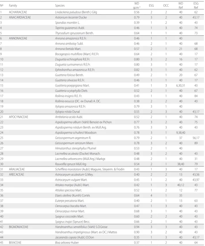
Table S1. List of species and their respective botanical families recorded in this study. Scientific names according to http://www.theplantlist.org/; WD – wood density in gcm-3; ESG – ecological species group: 1 – Pioneers, 2 – Early secondary, 3 – Late secondary/Climax, 4 – Exotic, 5 – Dead/Unknown; OCC – occurrence: 1 – Manaus, 2 – Santarem, 3 – Both; WD Ref – reference for wood density value; ESG Ref – reference for ecological species group.
Nº Family Species WD
gcm-3 ESG OCC WD Ref
ESG Ref
1 ACHARIACEAE Lindackeria paludosa (Benth.) Gilg 0.56 2 2 40 62
2 ANACARDIACEAE Astronium lecointei Ducke 0.79 3 2 40 43,17
3 Spondias mombin L. 0.39 1 2 40 43
4 Tapirira guianensis Aubl. 0.46 1 3 40 74
5 Thyrsodium spruceanum Benth. 0.64 1 1 40 73
6 ANNONACEAE Annona amazonica R.E.Fr. 0.46 1 1 40
7 Annona ambotay Subl. 0.46 2 1 40 68
8 Annona foetida Mart. 0.57 2 1 21 68
9 Bocageopsis multiflora (Mart.) R.E.Fr. 0.64 2 1 40 17
10 Duguetia echinophora R.E.Fr. 0.80 3 2 16 17
11 Duguetia surinamensis R.E.Fr. 0.80 3 1 40 17
12 Ephedranthus amazonicus R.E.Fr. 0.82 3 1 40 62
13 Guatteria foliosa Benth. 0.49 2 1 20 67
14 Guatteria olivacea R.E.Fr. 0.46 1 1 40 17
15 Guatteria poeppigiana Mart. 0.41 1 3 6,30,31 43
16 Guatteria scytophylla Diels 0.52 2 1 40 67
17 Rollinia insignis R.E. Fr. 0.43 1 1 40 84
18 Rollinia exsucca (DC. ex Dunal) A. DC. 0.38 2 2 40 43
19 Xylopia amazonica R.E.Fr. 0.79 3 1 40
20 Xylopia nitida Dunal 0.55 2 3 40 43,17
21 APOCYNACEAE Ambelania acida Aubl. 0.52 2 1 40 74
22 Aspidosperma album (Vahl) Benoist ex Pichon 0.77 3 2 40 75
23 Aspidosperma nitidum Benth. ex Müll.Arg. 0.76 3 3 40 43
24 Aspidosperma schultesii Woodson 0.78 3 1 9,38,40
25 Geissospermum argenteum R. 0.79 2 1 37 56,17
26 Geissospermum sericeum Miers 0.78 3 2 40 89
27 Himatanthus stenophyllus Plumel 0.53 2 1 40
28 Lacmellea aculeata (Ducke) Monach. 0.48 3 2 40 43
29 Lacmellea arborescens (Müll.Arg.) Markgr. 0.48 2 1 40 31
30 Rauvolfia sprucei Müll.Arg. 0.54 2 1 38,40 79
31 ARALIACEAE Schefflera morototoni (Aubl.) Maguire, Steyerm. & Frodin 0.43 1 3 40 17
32 ARECACEAE Astrocaryum aculeatum G.Mey. 0.40 2 2 13 43,56
33 Astrocaryum vulgare Mart. 0.45 1 2 40 43,97
34 Attalea maripa (Aubl.) Mart. 0.42 1 3 40,12 43
35 Attalea speciosa Mart. 0.52 1 2 12 77
36 Elaeis oleifera (Kunth) Cortés 0.64 4 1 35
37 Euterpe precatoria Mart. 0.40 2 1 13 63
38 Oenocarpus bacaba Mart. 0.47 1 3 40 43
39 Oenocarpus minor Mart. 0.68 3 1 40 43
40 Syagrus coccoides Mart. 0.60 2 2 40 43
41 Syagrus inajai (Spruce) Becc. 0.66 2 1 40 43
42 BIGNONIACEAE Handroanthus serratifolius (Vahl) S.O.Grose 0.94 3 3 40 43
43 Handroanthus impetiginosus (Mart. ex DC.) Mattos 0.90 3 2 40 43
44 Jacaranda copaia (Aubl.) D.Don 0.35 1 3 40 43,17
Nº Family Species WD
gcm-3 ESG OCC WD Ref
ESG Ref
46 BORAGINACEAE Cordia alliodora (Ruiz & Pav.) Oken 0.52 2 2 40 52,29
47 Cordia bicolor A.DC. 0.48 2 2 40 43,29
48 Cordia exaltata Lam. 0.40 1 1 40 43,75
49 Cordia goeldiana Huber 0.50 2 2 40 43,75
50 Cordia nodosa Lam. 0.39 2 1 40 31
51 BURSERACEAE Protium altsonii Sandwith 0.68 3 1 40 43
52 Protium hebetatum D.C. Daly 0.58 3 1 17 48
53 Protium heptaphyllum (Aubl.) Marchand 0.71 2 1 40 69,43
54 Protium paniculatum Engl. 0.65 3 2 40 47
55 Protium puncticulatum J.F. Macbr. 0.64 2 2 34 46
56 Protium robustum (Swart) D.M.Porter 0.68 2 2 16 56
57 Protium nitidifolium (Cuatrec.) D.C. Daly 0.62 2 1 20
58 Tetragastris altissima (Aubl.) Swart 0.71 2 2 40 65
59 Tetragastris panamensis (Engl.) Kuntze 0.73 3 1 40 43
60 Trattinnickia burserifolia Mart. 0.46 3 3 40 43
61 CANNABACEAE Trema micrantha (L.) Blume 0.25 1 3 40 51
62 CARICACEAE Jacaratia spinosa (Aubl.) A.DC. 0.14 2 2 31 88
63 CARYOCARACEAE Caryocar pallidum A.C.Sm. 0.84 3 1 40 17
64 Caryocar villosum (Aubl.) Pers 0.76 3 3 40 43
65 CHRYSOBALANACEAE Licania incana Aubl. 0.86 3 2 40 43
66 Licania micrantha Miq. 0.84 3 1 40 43
67 Licania oblongifolia Standl. 0.80 3 1 40 17
68 Licania prismatocarpa Spruce ex Hook.f. 0.84 3 1 9,38,40 67
69 CLUSIACEAE Symphonia globulifera L.f. 0.62 3 2 40 43
70 Tovomita brasiliensis (Mart.) Walp. 0.71 2 1 20 17
71 COMBRETACEAE Buchenavia macrophylla Spruce ex Eichler 0.82 3 1 38,40 17
72 CONNARACEAE Connarus perrottetii (DC.) Planch. 0.57 1 1 18 17
73 EBENACEAE Diospyros manausensis Cavalcante 0.72 3 1 38,40 31
74 ELAEOCARPACEAE Sloanea nitida G. Don 0.96 2 2 40 43
75 Sloanea laurifolia (Willd.) Benth. 0.82 2 1 40 43
76 EUPHORBIACEAE Aparisthmium cordatum (A.Juss.) Baill. 0.39 1 3 40 43
77 Croton sp. 0.47 1 2 40 17
78 Croton matourensis Aubl. 0.62 1 1 40 43
79 Glycydendron amazonicum Ducke 0.68 2 3 40 43
80 Hevea guianensis Aubl. 0.57 3 1 40 17
81 Hevea brasiliensis (Willd. ex A.Juss.) Müll.Arg. 0.40 3 3 40 43
82 Joannesia heveoides Ducke 0.39 2 2 40 78,47
83 Mabea angularis Hollander 0.61 2 1 38,40 17
84 Mabea speciosa Müll.Arg. 0.64 1 1 40 43
85 Mabea subsessilis Pax & K.Hoffm. 0.60 2 1 40 45
86 Maprounea guianensis Aubl. 0.59 1 1 40 43
87 Micrandra siphonioides Benth. 0.58 2 1 40 57,99
88 Nealchornea yapurensis Huber 0.61 3 1 40 76
89 Pausandra macropetala Ducke 0.59 2 1 37 79
90 Pogonophora schomburgkiana Miers ex Benth. 0.74 3 1 40 74,101,17
91 Sapium marmieri Huber 0.41 2 2 40 55
Nº Family Species WD
gcm-3 ESG OCC WD Ref
ESG Ref 93 FABACEAE CAESALPINIOIDEAE Apuleia leiocarpa (Vogel) J.F.Macbr. 0.80 3 2 40 31
94 Cassia leiandra Benth. 0.64 2 2 7 43,70
95 Chamaecrista xinguensis (Ducke) H.S.Irwin & Barneby 0.90 3 2 16
96 Crudia glaberrima (Steud.) J.F.Macbr. 0.79 2 2 40 43
97 Dimorphandra pennigera Tul. 0.75 3 1 40
98 Hymenaea courbaril L. 0.81 3 3 40 43
99 Hymenaea parvifolia Huber 0.88 3 2 40 43
100 Platymiscium duckei Huber 0.78 3 1 40 90
101 Schizolobium amazonicum Ducke 0.49 1 3 40 43
102 Tachigali paniculata var. alba (Ducke) Dwyer 0.55 1 2 31 43
103 Tachigali myrmecophila (Ducke) Ducke 0.48 3 2 40 43
104 Tachigali paniculata Aubl. 0.55 3 3 40 43
105 Tachigali setifera (Ducke) Zarucchi & Herend. 0.67 1 1 40 96
106 Tachigali venusta Dwyer 0.57 1 1 23 96
107 FABACEAE FABOIDEAE Andira parvifolia Benth. 0.92 3 1 40 17
108 Bowdichia nitida Benth. 0.80 3 2 40 43
109 Diplotropis martiusii Benth. 0.63 2 1 40 43
110 Diplotropis purpurea (Rich.) Amshoff 0.78 3 2 40 82
111 Diplotropis triloba Gleason 0.78 3 1 40 43
112 Dipteryx odorata (Aubl.) Willd. 0.92 3 3 40 43
113 Dipteryx punctata (S.F.Blake) Amshoff 0.92 3 1 40 89,102
114 Hymenolobium sericeum Ducke 0.72 3 1 20 43
115 Monopteryx inpae W.A.Rodrigues 0.74 3 1 40
116 Ormosia discolor Benth. 0.61 3 2 40 56
117 Ormosia flava (Ducke) Rudd 0.58 2 2 40 43
118 Ormosia nobilis var. santaremnensis (Ducke) Rudd 0.58 3 2 40 43
119 Ormosia paraensis Ducke 0.63 3 3 40 43
120 Poecilanthe parviflora Benth. 0.85 3 1 10, 4 80
121 Pterocarpus rohrii Vahl 0.46 2 1 40 17
122 Swartzia arborescens (Aubl.) Pittier 0.83 3 2 40 43
123 Swartzia cuspidata Benth. 0.68 3 1 40 67
124 Swartzia laevicarpa Amshoff 0.61 3 2 40 70
125 Swartzia polyphylla DC. 0.69 2 2 40 43
126 Swartzia recurva Poepp. 0.89 3 1 40 95
127 Swartzia schomburgkii Benth. 0.97 3 1 9 67
128 Sweetia nitens (Vogel) Yakovlev 0.80 3 2 40 59,47
129 FABACEAE MIMOSOIDEAE Abarema jupunba (Willd.) Britton & Killip 0.59 2 1 40 74,43
130 Alexa grandiflora Ducke 0.66 2 2 40 88
131 Dinizia excelsa Ducke 0.94 3 1 40 89
132 Enterolobium maximum Ducke 0.41 1 2 40 14
133 Enterolobium schomburgkii (Benth.) Benth. 0.72 3 3 40 64
134 Inga alba (Sw.) Willd. 0.59 2 3 40 29,74,56
135 Inga cayennensis Benth. 0.53 2 1 40 74
136 Inga gracilifolia Ducke 0.66 3 1 38,40 43
137 Inga macrophylla Willd. 0.68 3 1 2 43
138 Inga paraensis Ducke 0.82 3 1 40 74
139 Inga pilosula (Rich.) J.F.Macbr. 0.61 2 1 39 64
140 Inga rubiginosa (Rich.) DC. 0.66 3 2 40 43
Nº Family Species WD
gcm-3 ESG OCC WD Ref
ESG Ref
142 FABACEAE MIMOSOIDEAE Inga thibaudiana DC. 0.66 2 3 20 86,74,17
143 Marmaroxylon racemosum (Ducke) Record 0.84 3 2 40 47
144 Parkia gigantocarpa Ducke 0.26 1 2 40 85
145 Parkia multijuga Benth. 0.65 2 3 40 43
146 Parkia panurensis H.C.Hopkins 0.65 3 1 27 94
147 Parkia pendula (Willd.) Walp. 0.52 2 1 40 43,56
148 Pseudopiptadenia psilostachya (DC.) G.P.Lewis & M.P.Lima 0.61 3 3 16 43
149 Stryphnodendron pulcherrimum (Willd.) Hochr. 0.48 1 3 40 43
150 Stryphnodendron racemiferum (Ducke) W.A.Rodrigues 0.75 3 1 40
151 Stryphnodendron guianense (Aubl.) Benth. 0.57 2 1 40 17
152 Zygia racemosa (Ducke) Barneby & J.W. Grimes 0.75 3 1 40 17
153 GOUPIACEAE Goupia glabra Aubl. 0.73 2 3 40 43,56,17
154 HUMIRIACEAE Endopleura uchi (Huber) Cuatrec. 0.79 3 2 40 17
155 Sacoglottis mattogrossensis Malme 0.77 3 1 40 41
156 HYPERICACEAE Vismia cayennensis (Jacq.) Pers. 0.49 1 3 40 74
157 Vismia guianensis (Aubl.) Pers. 0.48 1 3 40 17
158 Vismia japurensis Rchb.f. 0.56 1 3 19 51
159 Vismia gracilis Hieron. 0.49 1 1 40 51
160 Vismia sandwithii Ewan 0.49 1 1 40 51
161 ICACINACEAE Emmotum acuminatum (Benth.) Miers 0.79 2 1 40 43
162 Poraqueiba sericea Tul. 0.91 3 1 8 8
163 LACISTEMACEAE Lacistema aggregatum (P.J.Bergius) Rusby 0.51 1 1 40 74
164 Lacistema grandifolium Schnizl. 0.52 1 1 40 74
165 LAMIACAEAE Vitex triflora Vahl 0.56 2 1 9 31
166 LAURACEAE Aniba burchellii Kosterm. 0.52 3 1 40 43
167 Aniba ferrea Kubitzki 0.52 3 1 9,38,40 17
168 Aniba panurensis (Meisn.) Mez 0.61 3 1 40 31
169 Aniba paraense Mez. 0.59 3 2 40 43,17,31
170 Dicypellium manausense W.A.Rodrigues 0.53 3 1 14 53
171 Endlicheria bracteata Mez 0.50 2 1 40 45
172 Licaria chrysophylla (Meisn.) Kosterm. 0.79 2 2 40 56
173 Mezilaurus ita-uba (Meisn.) Taub. ex Mez 0.74 3 2 40 43
174 Mezilaurus lindaviana Schwacke & Mez 0.68 2 2 40 71
175 Nectandra cuspidata Nees & Mart. 0.52 3 1 40 43
176 Ocotea baturitensis Vattimo-Gil 0.56 2 2 40
177 Ocotea canaliculata (Rich.) Mez 0.48 1 2 40 73
178 Ocotea cujumary Mart. 0.70 3 1 20 43
179 Ocotea glomerata (Nees) Mez 0.51 1 2 40 73
180 Ocotea guianensis Aubl. 0.53 3 1 40 43
181 Sextonia rubra (Mez) van der Werff 0.55 3 3 40 43
182 LECYTHIDACEAE Bertholletia excelsa Bonpl. 0.64 2 2 40 64
183 Corythophora rimosa W.A.Rodrigues 0.81 3 1 4 60
184 Couratari guianensis Aubl. 0.51 3 2 40 43
185 Eschweilera amazonica R.Knuth 0.90 3 2 40 43
186 Eschweilera atropetiolata S.A.Mori 0.75 3 1 40 17
187 Eschweilera bracteosa (Poepp. ex O.Berg) Miers 0.88 3 1 9 56
188 Eschweilera coriacea (DC.) S.A.Mori 0.85 3 3 40 43
189 Eschweilera obversa (O.Berg) Miers 0.83 3 2 40 82,43
190 Eschweilera wachenheimii (Benoist) Sandwith 0.81 3 1 40 82,43
191 Lecythis lurida (Miers) S.A.Mori 0.86 3 2 40 43
192 Lecythis pisonis Cambess. 0.86 3 2 40 43
193 Lecythis prancei S.A.Mori 0.88 3 1 40 43
Nº Family Species WD
gcm-3 ESG OCC WD Ref
ESG Ref
195 LINACEAE Roucheria columbiana Hallier f. 0.77 2 1 40 43
196 MALPIGHIACEAE Byrsonima chrysophylla Kunth 0.69 1 1 38,40 43
197 Byrsonima crispa A.Juss. 0.58 3 3 40 43
198 Byrsonima duckeana W.R.Anderson 0.69 3 1 38,40 84,17
199 MALVACEAE Apeiba echinata Gaertn. 0.36 1 3 31 88
200 Eriotheca globosa (Aubl.) A.Robyns 0.41 2 3 40 49
201 Luehea speciosa Willd. 0.52 2 2 25 43
202 Lueheopsis rosea (Ducke) Burret 0.33 2 1 40 56
203 Pachira glabra Pasq. 0.37 2 2 24 42
204 Quararibea ochrocalyx (K.Schum.) Vischer 0.56 2 1 20 88
205 Sterculia frondosa Rich. 0.47 1 1 40
206 Theobroma speciosum Willd. ex Spreng. 0.63 2 2 40 43
207 Theobroma sylvestre Aubl. ex Mart. in Buchner 0.67 2 1 40 17
208 MELASTOMATACEAE Bellucia dichotoma Cogn. 0.54 1 3 17 17
209 Bellucia grossularioides (L.) Triana 0.60 1 3 40 51
210 Miconia argyrophylla DC. 0.54 1 3 23 74,17
211 Miconia cuspidata Mart. ex Naudin 0.87 2 1 5 43
212 Miconia eriodonta DC. 0.63 1 1 2 74
213 Miconia poeppigii Triana 0.60 1 1 40 74
214 Miconia regelii Cogn. 0.60 2 1 38,40 68
215 Miconia serialis DC. 0.60 2 1 38,40 43
216 Miconia tetraspermoides Wurdack 0.60 2 1 38,40 31
217 Miconia tomentosa (Rich.) D.Don. 0.71 2 1 40 68
218 MELIACEAE Carapa procera DC. 0.68 2 2 40 74
219 Cedrela fissilis Vell. 0.47 2 2 40 14
220 Cedrela odorata L. 0.46 3 2 40 43
221 Guarea scabra A.Juss. 0.74 3 1 40 43,93
222 Trichilia septentrionalis C.DC. 0.53 3 1 29 43
223 MORACEAE Bagassa guianensis Aubl. 0.71 1 2 40 74,100
224 Brosimum rubescens Taub. 0.83 3 1 40 17
225 Brosimum acutifolium Huber 0.64 2 2 40 43
226 Brosimum guianense (Aubl.) Huber ex Ducke 0.84 2 2 40 69,29
227 Brosimum lactescens (S.Moore) C.C.Berg 0.66 2 2 40 29,75
228 Brosimum parinarioides Ducke 0.63 2 3 40 69
229 Clarisia racemosa Ruiz & Pav. 0.59 3 3 40 31
230 Ficus gomelleira Kunth & C.D.Bouché 0.39 2 1 22 31
231 Ficus nymphaeifolia Mill. 0.59 1 3 38,40,4 74
232 Ficus sp. 0.41 2 3 40 75
233 Helicostylis scabra (J.F.Macbr.) C.C.Berg 0.74 3 1 40 31
234 Helicostylis tomentosa (Poepp. & Endl.) J.F.Macbr. 0.63 2 1 40 43
235 Maquira sclerophylla (Ducke) C.C.Berg 0.51 1 3 40 43
236 Naucleopsis caloneura (Huber) Ducke 0.55 2 1 20,37 56
237 Perebea mollis (Poepp. & Endl.) Huber 0.37 2 2 40 82
238 MYRISTICACEAE Iryanthera grandis Ducke 0.63 3 2 40 31
239 Iryanthera juruensis Warb. 0.63 2 1 40 69,17
240 Osteophloeum platyspermum (Spruce ex A.DC.) Warb. 0.47 3 1 40 43
241 Virola multinervia Ducke 0.45 2 1 15 15
Nº Family Species WD
gcm-3 ESG OCC WD Ref
ESG Ref
243 MYRTACEAE Calyptranthes crebra McVaugh 0.78 2 1 40 56
244 Eugenia patrisii Vahl 0.83 3 1 40 70
245 Eugenia sp. 0.76 3 3 40 17
246 Myrcia fallax (Rich.) DC. 0.82 3 1 40 74
247 Myrcia guianensis (Aubl.) DC. 0.74 2 1 1 61
248 Myrcia magnoliifolia DC. 0.77 3 1 40
249 Myrcia paivae O.Berg 0.77 2 2 40 55
250 Myrcia sylvatica (G.Mey.) DC. 0.76 3 1 6 31
251 Myrciaria floribunda (H.West ex Willd.) O.Berg 0.79 3 3 40 88
252 NA Dead tree 0.34 5 3 3
253 NYCTAGINACEAE Neea madeirana Standl. 0.55 2 1 40 67
254 Neea oppositifolia Ruiz & Pav. 0.89 1 2 40 43,75
255 OLACACEAE Chaunochiton kappleri (Sagot ex Engl.) Ducke 0.52 2 1 40 43
256 Dulacia guianensis (Engl.) Kuntze 0.57 3 1 40 49
257 Minquartia guianensis Aubl. 0.80 3 1 40 43
258 OPILIACEAE Agonandra silvatica Ducke 0.83 3 1 40 62
259 PERACEAE Pera glabrata (Schott) Poepp. ex Baill. 0.67 1 1 40 43
260 PHYLLANTHACEAE Margaritaria nobilis L.f. 0.48 2 2 40 72
261 POLYGONACEAE Coccoloba latifolia Poir. 0.58 1 2 40 43
262 PROTEACEAE Roupala montana Aubl. 0.73 3 1 40 44,98
263 QUIINACEAE Lacunaria jenmanii (Oliv.) Ducke 0.92 3 1 38,40 56
264 Touroulia guianensis Aubl. 0.76 3 1 40
265 RUBIACEAE Capirona decorticans Spruce 0.59 2 2 40 96
266 Chimarrhis barbata (Ducke) Bremek. 0.71 2 1 40 62
267 Chimarrhis turbinata DC. 0.72 2 2 40 74
268 Coussarea ampla Müll.Arg. 0.48 2 1 40 83
269 Duroia longiflora Ducke 0.81 3 1 38 82,70
270 Genipa americana L. 0.62 1 2 40 43
271 Isertia hypoleuca Benth. 0.61 1 1 40 50
272 Palicourea corymbifera (Müll.Arg.) Standl. 0.66 1 1 38,40 92
273 Palicourea guianensis Aubl. 0.54 1 1 40 74
274 Fagara sp. 0.56 2 2 40 66
275 Zanthoxylum rhoifolium Lam. 0.57 2 3 40 43,56,17
276 SALICACEAE Casearia grandiflora Cambess. 0.77 2 1 40 31
277 Casearia javitensis Kunth 0.75 2 2 40 74
278 Casearia pitumba Sleumer 0.73 2 1 40 74,63
279 Casearia spruceana Benth. ex Eichler 0.68 2 2 40 75
280 Casearia ulmifolia Vahl ex Vent. 0.68 2 1 33,40 74,63,75
281 Laetia procera (Poepp.) Eichl. 0.63 2 3 40 74,51,17
282 Ryania speciosa Vahl 0.49 1 1 36
283 SAPINDACEAE Cupania hispida Radlk. 0.64 1 1 40 43
284 Matayba arborescens (Aubl.) Radlk. 0.70 1 1 40 43
285 Talisia carinata Radlk. 0.86 3 2 30
286 Talisia longifolia (Benth.) Radlk. 0.93 3 2 6 81
Nº Family Species WD
gcm-3 ESG OCC WD Ref
ESG Ref
288 SAPOTACEAE Manilkara bidentata (A.DC.) A.Chev. 0.87 3 1 40 43
289 Manilkara huberi (Ducke) Standl. 0.92 3 2 40 43
290 Micropholis casiquiarensis Aubrév. 0.71 3 1 40
291 Micropholis venulosa (Mart. & Eichler ex Miq.) Pierre 0.67 3 1 40 43
292 Pouteria bilocularis (H.J.P.Winkl.) Baehni 0.71 3 2 40 43
293 Pouteria gongrijpii Eyma 0.80 3 2 40 43
294 Pouteria guianensis Aubl. 0.93 3 1 40 43
295 Pouteria macrophylla (Lam.) Eyma 0.74 3 2 40 43
296 Pouteria oblanceolata Pires 0.79 3 1 40 17
297 Pouteria opposita (Ducke) T.D.Penn. 0.65 3 1 9 43
298 Pouteria petiolata T.D.Penn. 0.68 3 1 20 91
299 Pouteria platyphylla (A.C.Sm.) Baehni 0.80 3 1 28 43,70
300 Pouteria sp. 0.78 3 2 40 43,70
301 Pouteria torta (Mart.) Radlk. 0.77 2 2 40 87
302 Pouteria manaosensis Aubrév. & Pellegr. 0.64 3 1 15 17
303 SIMAROUBACEAE Simaba cedron Planch. 0.47 2 1 40 43
304 Simaba polyphylla (Cavalcante) W.W. Thomas 0.45 2 1 38 54
305 Simarouba amara Aubl. 0.38 2 1 40 74,17,56
306 SIPARUNACEAE Siparuna guianensis Aubl. 0.56 2 1 11 17
307 STRELITZIACEAE Phenakospermum guyannense (A.Rich.) Endl. 0.17 1 1 32 58
308 ULMACEAE Ampelocera edentula Kuhlm. 0.70 2 1 40 43
309 URTICACEAE Cecropia palmata Willd. 0.39 1 2 26 43
310 Cecropia purpurascens C.C.Berg 0.31 1 1 17 51,17
311 Cecropia sciadophylla Mart. 0.39 1 3 40 17
312 Pourouma guianensis Aubl. 0.38 1 3 40 74,43
313 Pourouma villosa Trécul 0.34 1 1 40 74,43
314 VIOLACEAE Rinorea guianensis Aubl. 0.78 2 3 40 17
315 Rinorea racemosa (Mart.) Kuntze 0.68 2 1 40 17
316 Rinorea pubiflora (Benth.) Sprague & Sandwith 0.75 3 2 40 55
317 VOCHYSIACEAE Erisma bicolor Ducke 0.70 3 1 27 75
318 Qualea paraensis Ducke 0.69 3 1 40 43
319 Qualea albiflora Warm. 0.57 3 1 40 43
320 Vochysia vismiifolia Spruce ex Warm. 0.75 3 1 27 43
321 Unknown 0.62 5 2
322 Unknown 0.62 5 2
323 Unknown 0.62 5 2
References
[1] Batalha, M.A.; Silva, I.A.; Cianciaruso, M.V.; França, H.; de Carvalho, G.H. 2011. Phylogeny, traits, environment, and space in Cerrado plant communities at Emas
National Park (Brazil). Flora: Morphology, Distribution, Functional Ecology of Plants, 206: 949–956.
[2] Block, A. 2004. Göttinger Mähhäcksler Tritucap und Forstmulcher- Nicht brennende Flächenvorbereitung am Beispiel der Zona Bragantina, Nord-Ost-Amazonien,
Brasilien. Georg-August-Universität, Göttingen, 219p.
[3] Chao, K.-J.; Phillips, O.L.; Baker, T.R. 2008. Wood density and stocks of coarse woody debris in a northwestern Amazonian landscape. Canadian Journal of Forest
Research, 38: 795–805.
[4] Chave, J.; Muller-Landau, H.C.; Baker, T.R.; Easdale, T.A.; Steege, H. ter; Webb, C.O. 2006. Regional and phylogenetic variation of wood density across 2456
neotropical tree species. Ecological Applications, 16: 2356–2367.
[5] Diniz, B.M. 2009. Relações hídricas e morfo-anatomia do caule em pares congenéricos do cerrado e mata de galeria: um estudo comparativo. Master’s thesis.
Universidade de Brasília, Brasília. 97p.
[6] Ducey, M.J.; Zarin, D.J.; Vasconcelos, S.S.; Araújo, M.M. 2009. Biomass equations for forest regrowth in the eastern Amazon using randomized branch sampling.