Airflow simulation in a horizontal closed refrigerated display cabinet

Vítor Hugo Moura Guedes

Airflow simulation in a horizontal closed

refrigerated display cabinet

Master’s Dissertation in Mechanical Engineer

Work developed under supervision of

Professor Doutor Pedro Alexandre Moreira Lobarinhas

Professora Doutora Senhorinha de Fátima Capela

Fortunas Teixeira

ii

DIREITOS DE AUTOR E CONDIÇÕES DE UTILIZAÇÃO DO TRABALHO POR TERCEIROS

Este é um trabalho académico que pode ser utilizado por terceiros desde que respeitadas as regras e boas práticas internacionalmente aceites, no que concerne aos direitos de autor e direitos conexos.

Assim, o presente trabalho pode ser utilizado nos termos previstos na licença abaixo indicada.

Caso o utilizador necessite de permissão para poder fazer um uso do trabalho em condições não previstas no licenciamento indicado, deverá contactar o autor, através do RepositóriUM da Universidade do Minho.

Licença concedida aos utilizadores deste trabalho

Atribuição CC BY

iii

A

CKNOWLEDGMENTS

To my tutors, Professor Pedro Lobarinhas, for all the knowledge and support provided, to Professor Senhorinha Teixeira, for the help and make me think a step ahead.

To Master João Vasconcelos, for following this project since its beginning and all the help especially with the software ANSYS – FLUENT.

To my family: my mother, my father and my brother, for making this project possible and all the support during it.

iv

D

ECLARAÇÃO DE INTEGRIDADE

Declaro ter atuado com integridade na elaboração do presente trabalho académico e confirmo que não recorri à prática de plágio nem a qualquer forma de utilização indevida ou falsificação de informações ou resultados em nenhuma das etapas conducente à sua elaboração.

Mais declaro que conheço e que respeitei o Código de Conduta Ética da Universidade do Minho.

v

R

ESUMO

Os equipamentos de refrigeração tornaram-se essenciais em várias vertentes, especialmente na conservação de alimentos. Nos últimos anos os equipamentos de refrigeração fechados têm ganho destaque devido ao seu consumo ser muito inferior comparativamente com os abertos.

O estudo centra-se na análise do escoamento de ar frio que percorre o equipamento, tendo em conta as condições exteriores. Para este efeito recorreu-se ao uso do programa CFD ANSYS Fluent. Este usa a técnica de volumes finitos na solução das equações de conservação da massa, momentum e energia.

Na primeira parte do trabalho fez-se um conjunto de simulações 2D em que foram estudados vários parâmetros. Primeiramente, foi analisada a dimensão da malha mais adequada (com apenas elementos quadriláteros); de seguida, foi feita uma comparação entre diferentes tipos de saídas e modelos de turbulência. Para terminar o estudo 2D foram colocados produtos de diferentes dimensões, atuando como obstáculos ao escoamento.

Quanto à influência dos parâmetros, pode concluir-se que o mais predominante é a temperatura na zona inferior junto ao evaporador. O fluxo de calor junto à parede e a influência das lâmpadas na geometria com produtos afetam pontualmente, não se refletindo noutras zonas geometria de uma forma evidente. O aumento da área perfurada nas costas na zona inferior permite uma maior ventilação nessa zona, contudo a temperatura aumenta ligeiramente.

Quanto à geometria com produtos, pode concluir-se através dos resultados que a geometria 2D utilizada é bastante limitadora.

vi

A

BSTRACT

Refrigeration equipment has become essential in several areas, especially in food preservation. In the last few years, closed refrigeration equipment becomes more popular because its consumption is much lower compared to the open ones.

The work of this study focuses on the analysis of the cold air flow that traverses the equipment, knowing the external conditions. For this purpose, CFD ANSYS Fluent program was used. This uses the finite volumes technique to solve the equations of conservation of mass, momentum and energy.

In the first part of the work, it was made a set of 2D simulations in which several parameters were studied. Firstly, the most appropriate mesh dimension was analysed (using only quadrilateral elements), then a comparison was made between different types of exits and turbulence models. To finish the 2D study products were introduced in the geometry with different dimensions, acting as obstacles to the fluid flow.

Concerning the influence of the parameters, it can be concluded that the most predominant is the temperature in the lower zone near the evaporator. The heat flux near the wall and the influence of the lamps on the geometry with products affect punctually, not being reflected in other geometry zones significantly. The increased perforated area in the lower back allows greater ventilation in the lower back, however the temperature increases slightly.

In the geometry with products, it can be concluded that the 2D geometry used is very limiting.

vii

C

ONTENTS

List of tables ... xii

Nomenclature ... xiii

List of symbols ... xiv

1. Introduction ... 1 1.1. Closed showcases ... 2 1.2. Objectives ... 3 1.3. Dissertation structure ... 4 2. State of art ... 6 2.1. Problem description ... 7

2.2. Cold equipment classification ... 8

2.3. Literature review ... 9 3. Computational model ... 15 3.1. Mathematical model ... 17 3.2. Turbulence models ... 24 3.3. Finite volumes ... 27 3.4. SIMPLE... 29

viii

3.5. Residual values and convergence ... 33

4. Case study ... 36

4.1. Strategies adopted ... 36

4.2. Mesh definition ... 38

4.3. Mesh optimization ... 40

5. Results and discussion ... 46

5.1. Study of some parameters influence ... 46

5.1.1. Boundary condition on the bottom boundary: 0°C ... 46

5.1.2. Heat flux 50 and 150W/m2_{K... 49}

5.1.3. Back entrances double size bottom ... 50

5.2. Geometry with products inclusion and lamps influence ... 52

6. Conclusion and future work ... 56

Conclusions ... 56

Future work ... 57

ix

L

IST OF FIGURES

Figure 1.1 - example of food preservation equipment ... 1

Figure 1.2 - cold showcase description ... 3

Figure 2.1 - showcase's full scheme, including the cold production zone and the storage zone ... 6

Figure 2.2 – Real steam compression system ... 7

Figure 2.3 - Temperature field using multiple air curtains ... 10

Figure 2.4 - mean temperature and standard deviations of the display cabinet with doors (a) and without doors (b)... 11

Figure 2.5 - Iced drink cabinet description, ... 12

Figure 2.6 - results at the end of each stage: (a) flow field, (b) temperature field ... 13

Figure 2.7 - Pathlines for plate evaporator, 1 - with a finned surface, 2 – without a finned surface ... 14

Figure 3.1 - Continuity on control volume, ... 18

Figure 3.2 - Conservation of momentum, ... 19

Figure 3.3 - Conservation of momentum in x ... 20

Figure 3.4 - Energy conservation, ... 23

Figure 3.5 – SST k-𝝎 model definition ... 26

Figure 3.6 -Fluxes in a 2D element according to finite volumes method ... 28

Figure 3.7 - Nodes and vector designation in a 2D element according to finite volumes method ... 29

Figure 3.8 - Control volume ... 31

Figure 3.9 - Residual values definition on ANSYS - FLUENT ... 35

x

Figure 4.2 - Mesh definition near the glass and wall, element size = 1.65mm (mesh 4, approximately 230,000 elements) ... 39 Figure 4.3 - Temperature field after 60s in the meshes 1 to 5, T0 = 15oC, v0 = 2 m/s, T(inlet)

= 0o_{C, Q(glass) = 8.29 W/m}2_{K ... 42}

Figure 4.4 - Velocity field after 60s in the meshes 1 to 5, T0 = 15oC, v0 = 2m/s, T(inlet) =

0o_{C, Q(glass) = 8.29W/m}2_{K ... 43}

Figure 4.6 - temperature field for mesh 3 after 60 seconds, T0 = 15oC, v0 = 2 m/s, T(inlet)

= 0o_{C, Q(glass) = 8.29 W/m}2_{K ... 45}

Figure 4.5 - temperature field for mesh 3 after 55 seconds, T0 = 15oC, v0 = 2m/s, T(inlet)

= 0o_{C, Q(glass) = 8.29 W/m}2_{K ... 45}

Figure 5.1 - definition of glass, inlet and outlet ... 47 Figure 5.2 – temperature field after 120s for meshes 4 and 5, T0 = 15oC, v0 = 2m/s, T(inlet)

= 0o_{C, Q(glass) = 8.29 W/m}2_{K, T(bottom) = 0}o_{C ... 47}

Figure 5.3 - velocity field after 120s for meshes 4 and 5, T0 = 15oC, v0 = 2 m/s, T(inlet) =

0o_{C, Q(glass) = 8.29 W/m}2_{K, T(bottom) = 0}o_{C ... 48}

Figure 5.4 – glass boundary condition ... 49 Figure 5.5 - temperature field after 120s, T0=15oC, v0 = 2 m/s, T(inlet) = 0oC, Q(glass) =

8.29 W/m2_{K, T(bottom) = 0}o_{C ... 50}

Figure 5.6 - temperature field after 120s, T0 = 15oC, v0 = 2 m/s, T(inlet)=0oC, Q(glass)=8.29

W/m2_{K, T(bottom) = 0}o_{C ... 50}

Figure 5.7 - velocity field after 120s, T0 = 15oC, v0 = 2 m/s, T(inlet) = 0oC, Q(glass) = 8.29

W/m2_{K, T(bottom) = 0}o_{C, with double sized entrances on the bottom of the perforated}

plate ... 51 Figure 5.8 - temperature field after 120s, T0 = 15oC, v0 = 2 m/s, T(inlet) = 0oC, Q(glass) =

8.29 W/m2_{K, T(bottom) = 0}o_{C, with double sized entrances on the bottom of the}

perforated plate ... 51 Figure 5.9 - geometry with products ... 52

xi

Figure 5.10 - mesh definition near the glass ... 53 Figure 5.11 - geometry with products, temperature field after 120s, T0 = 15oC, v0 = 2 m/s,

T(inlet) = 0o_{C, Q(glass) = 8.29 W/m}2_{K, T(bottom) = 0}o_{C, with double sized entrances on}

the bottom of the perforated plate ... 54 Figure 5.13 - geometry with products, velocity field after 120s, T0 = 15oC, v0 = 2m/s,

T(inlet) = 0o_{C, Q(glass) = 8.29 W/m}2_{K, T(bottom) = 0}o_{C, with double sized entrances on}

xii

L

IST OF TABLES

Table 2.1 - Classification of refrigerating equipment according to PRODCOM ... 8

Table 3.1 - Turbulence models description ... 25

Table 3.2 - Coefficients definition ... 32

xiii

N

OMENCLATURE

CFD Computational Fluid Dynamics

2D Two-dimensional

3D Three-dimensional

GWP Global Warming Potential

ODP Ozone Depletion Rate

xiv

L

IST OF SYMBOLS

𝜌 Density [kg/m3_]

𝜏 Surface stress [Pa]

S Source term [-]

q Heat flux [W/m2_]

K Turbulent kinetic energy [-]

T Temperature [K]

Re Reynolds number [-]

A Area [m2_]

𝑚̇ Mass flow [kg/s]

𝑘 Thermal conductivity coefficient [W/mK]

1

1. I

NTRODUCTION

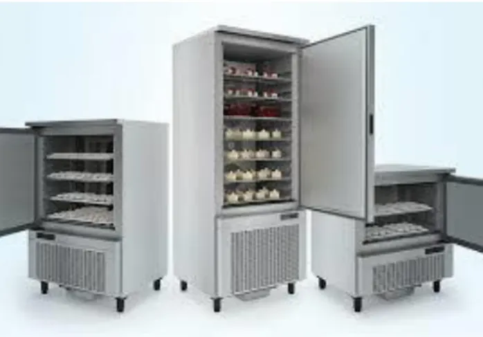
Mankind has always used food preservation since its inception. A very effective way of preserving food is to keep them at low temperatures, avoiding the formation of microorganisms, thus preventing their degradation. Over the years, several refrigeration systems have been created and refined for this purpose, the first of which consisted of simple cabinets with ice cubes. Even today the refrigeration is the most common process to preserve the food, although refrigeration has many other applications, such as health care, space cooling (to increase processes efficiency or comfort), industry, etc. (figure 1.1). There are many ways to «produce cold» and many fluids that can be used for this purpose. In the past many fluids were used because of their high efficiency (CFC, HCFC). However, some of them were banned because of the environmental impact. There are two main coefficients to evaluate this impact: ODP (Ozone Depletion Potential) and GWP (Global Warming Potential). Today the legislation only allows fluids with ODP equal to zero and low GWP (this value oscillate depending on the equipment, the application and if it is commercial or domestic).

Figure 1.1 - example of food preservation equipment, from http://ingecold.com.br/novidades_detalhe.php?noticia=24

As already mentioned, the main concern nowadays with the use of cold equipment has to do with its energy expenditure. This implies the correct use of equipment (such as reducing the opening time of doors in a refrigerator/freezer), but

2

also a greater effort on the part of the manufacturers, who must guarantee the correct functioning of the equipment with the minimum power dissipated. For that reason, closed display cabinets become more and more popular over the years[1].

The most popular way to produce cold in these devices is using refrigerants, that will transport the heat from the cold source to the hot source. Depending on which source is the one is interested (to refrigerate is the cold source and to heating is the hot source), there are two different classifications: heat pumps (heating) and refrigeration machines (cooling). That the operation is the same for both, and there are many types of equipment that can do both tasks, such as air conditioners.

1.1. Closed showcases

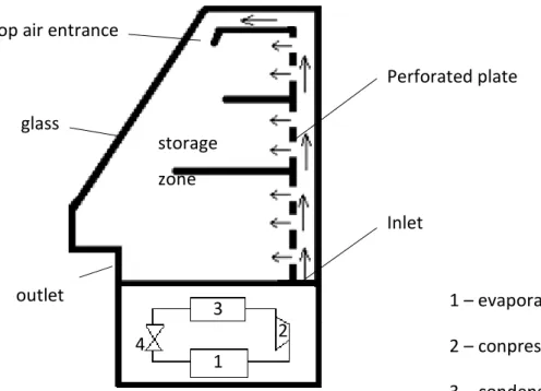
Commercial refrigeration equipment is indispensable for the preservation of food in such establishments, namely butchers, bakeries, etc. A schematic drawing of the cabinet is presented in figure 1.2. There is an upwards airflow on the back that will be split in two: a fraction of this flow is entering on the equipment by the back perforated plated and the rest of it is entering on the top, near the glass on the front, forming an air curtain.

This type of equipment is divided into two zones: cold production and storage (figure 1.2). The cold production zone is usually located at the bottom of the equipment. This zone contains insulating material to prevent energy loss to the outside and there is only one connection to the storage zone to enable the airflow.

3

Figure 1.2 - cold showcase description

Air enters the storage area through the back of the showcase (through a perforated plate) and through an existing channel on the top. Afterwards, the air is exhausted from the bottom of the storage zone, entering the cold production zone again, starting a new cycle. The existence of a perforated plate is crucial to ensure uniformity of flow in the storage zone. This area is bounded by a glass on the face that is customer-facing because the glass is a transparent material to facilitate customer choice. If there is a freezing zone, it is not visible, and it is attached to the cold production zone.

It is also common that in the storage zone there are different temperatures intended for different foods, even in equipment without freezing.

1.2. Objectives

As referred before, the main goal is to optimize the showcase in order to reduce its consumptions without compromising its purpose. There are 2 methods to evaluate this kind of situations: computational and experimental. The computational method is an extension of the mathematical, but its faster and it is easier to visualise the problem. The main reason for using CFD as a tool to optimize the equipment is the reduced cost

Top air entrance

Perforated plate glass storage zone outlet Inlet 3 1 – evaporator 2 – conpressor 3 – condenser 4 – expansion valve 4 2 1

4

and time when compared to experimental studies. So, the project should follow this schedule:

• Modelling a closed display cabinet

• Study of the flow in a closed display cabinet in order to determine the following parameters:

- The temperature range inside it, so that this range of values is the smallest possible and that these temperatures allow the preservation of food.

- The flow velocity so that it does not exceed a certain value (so that it does not produce excessive noise and does not dehydrate the food)

- Study the influence of different parameters and the relative importance of each one. - Influence of the heat flux from all sources, namely heat transfer from the exterior through the boundaries and dissipated power from electric devices (for example the lamps).

- Influence of the products in the refrigerating process. 1.3. Dissertation structure

Considering the objectives mentioned before, in the next chapter the problem will be contextualized, explaining the origin of the cold air entering the storage zone. Some classifications of this type of equipment will be presented according to different entities, and finally a brief literature review including CFD and experimental work.

Chapter 3 will introduce numerical simulation and the software ANSYS-Fluent used for this project, considering some calculation strategies included on it and its functionalities.

In chapter 4, the case study will be presented, including the geometry, mesh definition and mesh optimization. It will be explained how to optimize the mesh to the study.

In chapter 5, the influence of several parameters will be studied. The last case studied will include products, for which a new geometry and mesh will be needed. For each model, there will be a small explanation of why this model was made and the next step of the study.

5

Finally, the last chapter will draw some conclusions and propose some future work that can continue this research.

6

2. S

TATE OF ART

In this chapter, the problem will be described, and the equipment will be presented and its working process. Then it will be presented the legislation to this kind of equipment and its classification considering the properties and operation parameters. Lastly, some scientific papers and other works similar to this one will be reviewed.

Figure 2.1 presents the full showcase, with the cold production zone and the storage zone.

Figure 2.1 - showcase's full scheme, including the cold production zone and the storage zone

The next subchapter explains how the cold is produced in this kind of equipment. However, in the present study, this process will be ignored and it will be considered only the storage zone.

4 3 2 1 1 – evaporator 2 – compressor 3 – condenser 4 – expansion valve storage zone

7

2.1. Problem description

The most common system used in the showcases to produce cold is by vapour compression (figure 2.2)

Figure 2.2 – Real steam compression system[2]

At point 1, the refrigerant is in a state of superheated vapour (in an ideal cycle, it would be saturated steam, but in the real case it is not to guarantee that there is no liquid in the compressor). Then there is a compression in order to raise the temperature and pressure of the refrigerant before the condenser, which will remove heat from the fluid. At this stage, the energy from the refrigerant can/should be used to warm the environment or another process in order to monetize all the energy (most important step of the heat pump). The refrigerant at the end of the condenser is liquid (similarly the liquid is subcooled to guarantee there is no gas on the expansion). Then there is an expansion valve before the refrigerant enters in the evaporator when it will be heated by the refrigerated space, restarting another cycle. This refrigerated space will be the study object of this project.

8

There are many other systems used in certain situations that will not be analysed because they are not relevant in this case[3].

Therefore, the main goal of this project is the improvement of the efficiency in a showcase, that is reducing the consumptions without compromising its purpose. The consumption reduction is achieved by lowering the mass flow rate and/or increasing the air inlet temperature (reducing the power of the refrigeration system). In order to optimize the equipment, the temperature field will be evaluated inside the showcase, maintaining the inlet conditions.

2.2. Cold equipment classification

Thus, several classifications were assigned according to their application and operating parameters. According to the European Community PRODCOM (from the French 'PRODuction COMmunautaire'), the cold store can be fitted in the code 'CPA 29.23.13: Refrigerating and freezing equipment (table 2.1) and heat pumps, except household type equipment', which can be divided into several subgroups [4]:

Table 2.1 - Classification of refrigerating equipment according to PRODCOM

Code Description Characteristics

29.23.13.33 Refrigerated show-cases and counters incorporating a refrigerating unit or evaporator for frozen food storage

Refrigerated and frozen food

29.23.13.35 Refrigerated show-cases and counters incorporating a refrigerating unit or evaporator (excluding for frozen food storage)

Refrigerated good

29.23.13.40 Deep-freezing refrigerating furniture (excluding chest freezers of a capacity ≤ 800 litres, upright freezers of a capacity ≤ 900 litres)

Frozen food, small equipment

9

29.23.13.50 Refrigerating furniture (excluding for deep-freezing, show-cases and counters incorporating a refrigerating unit or evaporator)

Frozen food, large equipment

29.23.13.90 Other refrigerating and freezing equipment

The equipment under analysis is a commercial showcase that does not contain frozen food storage, so, considering this classification, this furniture fits in group 29.23.13.35.

There are many other entities using other classifications, such as EUROVENT, US Department of Energy, Energy Star Program requirements, etc. that are more precise, considering the following specifications:

• Volume

• Operating temperature:

- Refrigeration (temperature higher than 0°C) - Freezing (temperature bellow 0°C)

- Combined refrigeration and freezing

• Vertical or horizontal

• Self-contained or remote compression

• With or without doors, material (solid doors or glass)

• Opening type: sliding or pivoting.

The normative EN ISO 23953 classifies equipment according to their orientation (vertical, semi-vertical or horizontal), shape (line-up, islands, etc), operating temperature, service type (self-service or assisted service).

2.3. Literature review

Ribeiro et al (2016) [5] developed a numerical study (2D) using 3 different models of an open vertical display cabinet: the first one using a simple air curtain, the second one using deflection blades and the third one using multiples air curtains. These curtains

10

are refrigerated by the evaporator on the bottom. The air velocity was defined at the exit of the evaporator. This study surprisingly obtained better results on the first model (figure 2.3); however, it refers that the second one has more potential if the deflection blades were optimized. According to the author, the third model was not successful because of the increment of complexity. These results have natural limitations due to being performed in 2D simulations.

Figure 2.3 - Temperature field using multiple air curtains[5]

Chaomuang et al. (2019) developed an experimental study of a closed display cabinet, where the main goals were analysing the factors that influence the temperature inside the equipment and its variation, comparing these results with the same cabinet but with the doors opened (figure 2.4)[6]. The authors observed that 70% of the heat transfer was due to thermal bridges and gaps (for example the air infiltration between the doors). Comparing the temperatures with and without doors (when the cabinet was empty), in the storage zone there was an increment from 0.4 to 3.1°C and from 8.2 to 9.5°C in the shelf edges (near the air curtain). The influence of ambient temperature was

11

also studied: the authors verified that there is an almost linear relationship between the air temperature inside the equipment and the external temperature.

Figure 2.4 - mean temperature and standard deviations of the display cabinet with doors (a) and without doors (b),

[6]

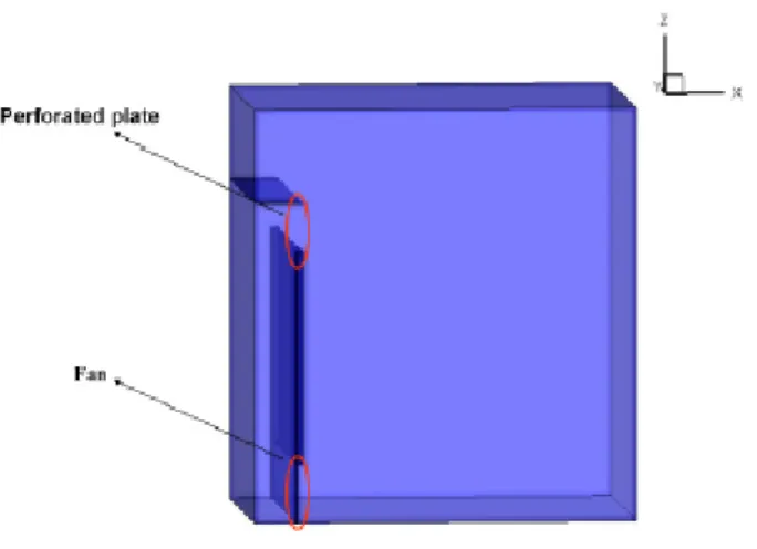
Wang et al. (2015) developed a numerical 3D study of an iced drink refrigeration cabinet, where the temperatures inside fluctuate between -7°C and -5°C, using an automated switch on and automated switch off [7].

The cabinet has an enclosing perforated plate that separates the evaporator and the storage room, which is simulated by the porous jump model. In the coolant air chamber, there is a fan in the bottom to assist the air circulation (figure 2.5).

12

Figure 2.5 - Iced drink cabinet description, (Wang et al., 2016)

The first time the switch turns on, the refrigeration cabinet is at the same temperature of the room, 25°C. The switch remains on until the temperature reaches the lower limit, -7°C (first stage). Then the switch turns off and the temperature inside the cabinet will naturally raise due to the room temperature being higher until the temperature is -5°C (second stage), when the switch turns on, starting a new cycle (third stage). The authors conclude that in order to obtain satisfying results they had to simulate the full process (figure 2.6).

13

Figure 2.6 - results at the end of each stage: (a) flow field, (b) temperature field, [7]

Belman-Flores et al. (2016) built up a numerical study in order to analyse the temperature and flow in a refrigerator [8]. Its dimensions are 0.4m × 0.35m × 0.50m (width, depth, height) and use three different fluids for the cooling system: ammonia, water and hydrogen, which are the refrigerant, absorbent and auxiliary gas, respectively. The authors main objective was analysing the conditions on the compartment food storage (temperature and velocity) and compared it in different conditions, such as shelf position (top and bottom) and with or without finned surface (figure 2.7)

14

Figure 2.7 - Pathlines for plate evaporator, 1 - with a finned surface, 2 – without a finned surface, [8]

They concluded that there is a difference in the average temperature of 0.7K, which means that the model without a finned surface is an acceptable option. In terms of energy consumption, both models have similar results. This model can still have great improvements with an optimal geometry of the plate evaporator.

2

1

15

3. C

OMPUTATIONAL MODEL

Fluid flows are governed by partial differential equations that represent the laws of conservation of mass, momentum and energy. CFD includes fluid mechanics, numerical analysis and computational science, transforming the partial differential equations into systems of algebraic equations with solution algorithms that calculate the value of the desired variables.

The computational analysis can be divided into 3 components: pre-processing, solver and post-processing. Pre-processing involves all the preparation and conditions definition needed for the calculation, such as geometry, mesh and boundary conditions. Solver includes the calculation of all variables intended for the study. On post-processing, the results are analysed in many different ways, such as contours, vector graphics, video, etc.

Pre-Processing

At this stage, the physical problem is defined by adapting itself to the treatment of the solver. Pre-Processing is divided into the following phases:

• Geometry and problem’s domain definition;

• Mesh creation is the division of the geometry in control volumes; • Selection of physical phenomenon to study.

• Definition of fluid properties and boundary conditions

The solution of the problem is defined on the nodes in the interior of each control volume since the precision of the solution is directly related to the refinement of the mesh. That is if a mesh is refined the result of the simulations for greater accuracy. However, there is a maximum accuracy that can be achieved, so the mesh should be optimized in order to save computational time. The control volume should be as small as possible in areas where there is a more abrupt change in flow properties while in areas where there is no such change in fluid properties the volume of the control may already be larger (for example: in the simulation of the laminar flow of a fluid in a pipeline the mesh must be more refined next to the walls of the pipeline since it is in

16

that zone where there will be a greater variation of the flow rate, whereas when approaching the axis of the pipeline the mesh does not need to be so refined).

Solver

In Fluent there are two numerical methods based on the finite volume technique: pressure-based and density-based solver. The first is used for problems in which the flows are incompressible and at low speed while the second one is more suitable for studies of compressible flow and high speed. In both cases, the velocity value is given by the momentum equation. In the first method, the density is obtained through the equation of continuity, while the other method the solution of the pressure field is given by the manipulation of the equation of continuity with the momentum equation.

Both methods follow these steps:

• Initially, the previously defined mesh is divided into discrete control volumes. • Integration of the equations into each control volume, thus constructing the discrete algebraic equations of dependent variables (the ones to be calculated), such as velocity, temperature, pressure, and so on.

• Linearization of the discretized equations and solution resulting from the system of linear equations of the dependent variables.

Post-processing

ANSYS Fluent Software has a wide range of graphic capabilities in the post-processing interface, including:

• Visualization of geometry and mesh;

• Vector graphics;

• Coloured contours and flow lines

• Particles trajectory;

• Images manipulation;

17

3.1. Mathematical model

The main equations of the mathematical model are the mass conservation law, continuity and energy equation:

Mass conservation law (continuity equation)

This law is based on the mass balance in the element, that means that the mass variation in the control volume is equal to the net change in mass in the control volume. The net change is the difference between the mass entering each face is the same as that which exits on the opposite side of that control volume. So, the mass variation in the control volume is given by:

𝜕

𝜕𝑡(𝜌𝛿𝑥𝛿𝑦𝛿𝑧) =

𝜕𝜌

𝜕𝑡(𝛿𝑥𝛿𝑦𝛿𝑧) 3.1

In turn, the mass passing through each face of the control volume is given by the product of the density and the velocity in the component normal to the face of the control. Let u, v and w be the velocities along the x, y, and z axes respectively. Figure 3.1 shows the mass flows in the control volume, which is given by:

(𝜌𝑢 −𝜕𝜌𝑢 𝜕𝑥 1 2𝜕𝑥) 𝛿𝑦𝛿𝑧 − (𝜌𝑢 − 𝜕𝜌𝑢 𝜕𝑥 1 2𝜕𝑥) 𝛿𝑦𝛿𝑧 + (𝜌𝑣 −𝜕𝜌𝑣 𝜕𝑦 1 2𝜕𝑦) 𝛿𝑥𝛿𝑧 − (𝜌𝑣 − 𝜕𝜌𝑣 𝜕𝑦 1 2𝜕𝑦) 𝛿𝑥𝛿𝑧 + (𝜌𝑤 −𝜕𝜌𝑤 𝜕𝑧 1 2𝜕𝑧) 𝛿𝑥𝛿𝑦 − (𝜌𝑤 − 𝜕𝜌𝑤 𝜕𝑧 1 2𝜕𝑧) 𝛿𝑥𝛿𝑦 3.2

18

Figure 3.1 - Continuity on control volume, [9]

Adding the transient term and dividing all terms by δxδyδz: 𝜕𝜌 𝜕𝑡 + 𝜕𝜌𝑢 𝜕𝑥 + 𝜕𝜌𝑣 𝜕𝑦 + 𝜕𝜌𝑤 𝜕𝑧 = 0 3.3

The last equation represents the mass conservation of three-dimensional transient flow in a compressible fluid. The first term represents the term transient while the others represent the term convective

Momentum conservation law (momentum equation)

According to Newton's 2nd law F = ma, the momentum in the control volume

particle is equal to the sum of the forces in the particle. The variation of momentum in the x, y, and z axes per unit volume in the control volume is given by:

𝜌𝐷𝑢 𝐷𝑡 𝑖𝑛 𝑥 ; 𝜌 𝐷𝑣 𝐷𝑡 𝑖𝑛 𝑦; 𝜌 𝐷𝑤 𝐷𝑡 𝑖𝑛 𝑧 3.4

19

There are two types of forces in the control volume: • Surface forces

- Forces due to pressure - Forces due to viscosity

• Body forces

- Forces due to gravity - Centrifugal forces - Coriolis forces

- Electromagnetic forces

Surface forces will be considered in terms of momentum and the body forces contained in the source term.

In a three-dimensional case, the stress state in the fluid element is defined in terms of pressure and nine components of viscosity stresses as shown in Figure 3.2. The pressure is identified by the letter p and the viscous stress by the letter τ.

Figure 3.2 - Conservation of momentum, [9]

Considering that the forces on the components in x resulting from the pressure

p and the surface stresses τxx, τxy and τxz, (Figure 3.3). The resulting force in x is the

20

Figure 3.3 - Conservation of momentum in x, [9]

The resulting forces in x on the faces (E, W) are:

[(𝑝 −𝜕𝑝 𝜕𝑥 1 2𝛿𝑥) − (𝜏𝑥𝑥− 𝜕𝜏_𝑥𝑥 𝜕𝑥 1 2𝛿𝑥)] 𝛿𝑦𝛿𝑧 + [− (𝑝 −𝜕𝑝 𝜕𝑥 1 2𝛿𝑥) − (𝜏𝑥𝑥− 𝜕𝜏_𝑥𝑥 𝜕𝑥 1 2𝛿𝑥)] 𝛿𝑦𝛿𝑧 = (−𝜕𝑝 𝜕𝑥+ 𝜕𝜏_𝑥𝑥 𝜕𝑥 ) 𝛿𝑥𝛿𝑦𝛿𝑧 3.5

In faces (N, S) in the x-axis results:

− (𝜏_𝑦𝑥−𝜕𝜏𝑦𝑥 𝜕𝑦 1 2𝛿𝑦) 𝛿𝑥𝛿𝑧 + (𝜏𝑦𝑥− 𝜕𝜏_𝑦𝑥 𝜕𝑦 1 2𝛿𝑦) 𝛿𝑥𝛿𝑧 = 𝜕𝜏_𝑦𝑥 𝜕𝑦 𝛿𝑥𝛿𝑦𝛿𝑧 3.6

Lastly, the forces on direction x on faces (T, B) are given by:

− (𝜏_𝑧𝑥−𝜕𝜏𝑧𝑥 𝜕𝑧 1 2𝛿𝑧) 𝛿𝑥𝛿𝑦 + (𝜏𝑧𝑥− 𝜕𝜏_𝑦𝑥 𝜕𝑧 1 2𝛿𝑧) 𝛿𝑥𝛿𝑦 = 𝜕𝜏_𝑧𝑥 𝜕𝑧 𝛿𝑥𝛿𝑦𝛿𝑧 3.7

21

The total force by volume unit of the fluid resulting from the surface tensions is obtained by the sum of equations mentioned above, which divided by δxδyδz results:

𝜕(−𝑝 + 𝜏_𝑥𝑥) 𝜕𝑥 + 𝜕𝜏_𝑦𝑥 𝜕𝑦 + 𝜕𝜏_𝑧𝑥 𝜕𝑧 3.8

The equation of momentum in component x is obtained by the equality of the momentum variation with the resultant of the force due to the surface tensions of the equation (previous equation) plus the term source in x.

𝜌𝐷𝑢 𝐷𝑡 = 𝜕(−𝑝 + 𝜏𝑥𝑥) 𝜕𝑥 + 𝜕𝜏_𝑦𝑥 𝜕𝑦 + 𝜕𝜏𝑧𝑥 𝜕𝑧 + 𝑆𝑀𝑥 3.9

Similarly, on the y component:

𝜌𝐷𝑣 𝐷𝑡 = 𝜕(−𝑝 + 𝜏_𝑦𝑦) 𝜕𝑦 + 𝜕𝜏_𝑦𝑥 𝜕𝑥 + 𝜕𝜏_𝑧𝑦 𝜕𝑧 + 𝑆𝑀𝑦 3.10 And z component: 𝜌𝐷𝑤 𝐷𝑡 = 𝜕(−𝑝 + 𝜏_𝑧𝑧) 𝜕𝑧 + 𝜕𝜏𝑦𝑧 𝜕𝑦 + 𝜕𝜏_𝑧𝑥 𝜕𝑥 + 𝑆𝑀𝑧 3.11

Energy conservation law (Energy equation)

This equation is derived from the first law of thermodynamics which states that the internal rate of change of a fluid particle is the sum of the variation of heat and the variation of the work.

Saying that the variation rate 𝜌 is given by:

𝜌𝐷𝐸

22

Work is equal to the product of force by the component of velocity in the direction of the force. Making the product of equation 3.9 with the velocity in the component in x: 𝜕𝑢(−𝑝 + 𝜏_𝑥𝑥) 𝜕𝑥 + 𝜕(𝑢𝜏𝑦𝑥) 𝜕𝑦 + 𝜕(𝑢𝜏_𝑧𝑥) 𝜕𝑧 3.13

The same happens with y and z components, obtaining respectively: 𝜕𝑣(−𝑝 + 𝜏_𝑦𝑦) 𝜕𝑦 + 𝜕(𝑣𝜏_𝑥𝑦) 𝜕𝑥 + 𝜕(𝑣𝜏_𝑧𝑦) 𝜕𝑧 3.14 𝜕𝑤(−𝑝 + 𝜏𝑧𝑧) 𝜕𝑧 + 𝜕(𝑤𝜏_𝑦𝑧) 𝜕𝑦 + 𝜕(𝑤𝜏𝑥𝑧) 𝜕𝑥 3.15

Isolating the terms that contain pressure p:

−𝜕(𝑢𝑝) 𝜕𝑥 − 𝜕(𝑣𝑝) 𝜕𝑦 + 𝜕(𝑤𝑝) 𝜕𝑧 = −𝑑𝑖𝑣(𝑝𝑢) 3.16

The total work variation resulting from the superficial forces is given by:

[−𝑑𝑖𝑣(𝑝𝑢)] + [ 𝜕(𝑢𝜏𝑥𝑥) 𝜕𝑥 + 𝜕(𝑢𝜏_𝑦𝑥) 𝜕𝑦 + 𝜕(𝑢𝜏𝑧𝑥) 𝜕𝑧 ] + [ 𝜕(𝑣𝜏𝑥𝑦) 𝜕𝑥 + 𝜕(𝑣𝜏_𝑦𝑦) 𝜕𝑦 + 𝜕(𝑣𝜏_𝑧𝑦) 𝜕𝑧 ] + [ 𝜕(𝑤𝜏𝑥𝑧) 𝜕𝑥 + 𝜕(𝑤𝜏𝑦𝑧) 𝜕𝑦 + 𝜕(𝑤𝜏_𝑧𝑧) 𝜕𝑧 ] 3.17

Equation 3.17 represents the balance of all x, y, and z components of work on the fluid particle resulting from forces acting on surfaces.

23

The balance of the heat flux through the faces of the control volume is represented by the vector of heat flow q in the three components qx, qy and qz, according

to Figure 3.4.

Figure 3.4 - Energy conservation,[9]

[(𝑞_𝑥−𝜕𝑞𝑥 𝜕𝑥 1 2𝛿𝑥) − (𝑞𝑥+ 𝜕𝑞_𝑥 𝜕𝑥 1 2𝛿𝑥)] 𝛿𝑦𝛿𝑧 = − 𝜕𝑞_𝑥 𝜕𝑥 𝛿𝑥𝛿𝑦𝛿𝑧 3.18

The same happens for the components y and z.

−𝜕𝑞𝑦

𝜕𝑦 𝛿𝑥𝛿𝑦𝛿𝑧 _3.19

−𝜕𝑞𝑧

𝜕𝑧 𝛿𝑥𝛿𝑦𝛿𝑧

3.20

Dividing the equations above by δxδyδz:

−𝜕𝑞𝑥 𝜕𝑥 − 𝜕𝑞_𝑦 𝜕𝑦 − 𝜕𝑞_𝑧 𝜕𝑧 = −𝑑𝑖𝑣 𝑞 3.21

24

According to the Fourier law for the heat flow by conduction:

𝑞_𝑥− 𝐾𝜕𝑇 𝜕𝑥; 𝑞𝑦 − 𝐾 𝜕𝑇 𝜕𝑦; 𝑞𝑧− 𝐾 𝜕𝑇 𝜕𝑧 3.22

That can be expressed by:

𝑞 = −𝑘𝑔𝑟𝑎𝑑 𝑇 3.23

Combining the two previous equations, the final energy balance equation is obtained resulting from the conduction heat transfer process.

−𝑑𝑖𝑣 𝑞 = 𝑑𝑖𝑣 (𝑘 𝑔𝑟𝑎𝑑 𝑇) 3.24

3.2. Turbulence models

Most flows studies are turbulent studies. A flow is defined as laminar, intermediate or turbulent through the Reynolds number. This number is given by the ratio of inertial forces to viscous forces (UL / ν). Since U is the velocity of the fluid, L is the characteristic length of the flow, and ν is the kinematic viscosity. For low values of the Reynolds number the flow is laminar, above the critical value (transient Reynolds value) the flow becomes turbulent.

The ANSYS fluent software uses an approach to the numerical simulation names RANS (Reynolds Averaged Navier-Strokes Simulation) [10]. This technique solves time-averaged Navier-Strokes equations and offers several methods of turbulence for all turbulent length. This is the most common approach in the industry due to his low cost compared to other ones (DNS, LES). There are many turbulent models that can be used in this approach, which must be chosen considering the Reynolds number, fluid properties and its application (Table 3.1).

25

Model Behaviour and usage

Spalart-Allmaras

Economical for large meshes. Performs poorly for 3D flows, free shear flows, flows with strong separation. Suitable for mindly complex (quasi-2D) external/internal flows and boundary layer flows under pressure gradient (e.g. airfoils, wing, airplane fuselages, missiles, ship hulls

Standard k- 𝜺

Robust. Widely used despite the known limitations of the model. Performs poorly for complex flows involving severe pressure gradient, separation, strong streamline curvature. Suitable for initial screening or alternative designs, and parametric studies

Realizable k- 𝜺

Suitable for complex shear flows involving rapid strain, moderate swirl, vortices, and locally transitional flows (e.g. boundary layer separation, massive separation and vortex shedding behind bluff bodies, stall in wide-angle diffusers, room ventilation).

RNG k- 𝜺 Offers largely the same benefits and has similar applications as Realizable. Possibly harder to converge than realizable.

Standard k- 𝝎

Superior performance for wall-bounded boundary layer, free shear, and low Reynolds number flows. Suitable for complex boundary layer flows under adverse pressure gradient and separation (external aerodynamics and turbomachinery). Can be used for transitional flows (thought tends to predict early transition). Separation is typically predicted to be excessive early

SST k- 𝝎 Offers similar benefits as standard k- 𝜔. Dependency on wall distance makes this less suitable for free shear flows.

26

There will be studied two different models, Realizable k-𝜀 and SST k-𝜔, which can be the most suitable for this study and its variations.

Turbulence model Realizable k-𝜺 (RKE)

This model, like the Standard k-𝜀 (SKE) model, is suitable for most situations but has some benefits compared to the previous one, such as:

• Accurately predicts the spreading rate of both planar and round jets.

• Also, likely to provide superior performance for flows involving rotation, boundary layers under strong adverse pressure gradients, separation, and recirculation.

It is expected to have some rotation in this case study, that is the main reason the SKE was excluded for this situation.

Turbulence model SST k-𝝎

k-𝜔 models have better performance for boundary layer flows and low Reynolds number flows. SST k-𝜔 specifically, is a mix of a k-𝜔 model near the wall and k-𝜀 in the freestream (Figure 3.6).

Figure 3.5 – SST k-𝝎 model definition[10] RSM

Physically the most sound RANS model. Avoids isotropic eddy viscosity assumption. More CPU time and memory required. Tougher to converge due to close coupling of equations. Suitable for complex 3D flows with strong streamline curvature, strong swirl/rotation (e.g. curved duct, rotating flow passages, swirl combustors with very large inlet swirl, cyclones).

27

This model is a good compromise between k-𝜔 and k-𝜀 models. Near wall treatment

Four different models can be chosen in order to define the flow behaviour near the wall: Standard wall functions, Non-equilibrium wall functions, Enhanced wall treatment, User-Defined Wall functions.

As it was done in the turbulence models, standard wall functions and enhanced wall treatment models will be considered.

Standard wall functions model is designed for high Re attached flow, the near-wall region is not resolved, the near-near-wall mesh is relatively coarse.

The enhanced wall treatment model is used for low Re flows or flows with near-wall complex phenomena. Usually requires a very-fine near-near-wall mesh capable of resolving this region but can also handle coarse near-wall mesh.

3.3. Finite volumes

The finite volume method uses as a starting point the integral form of the conservation equation.

The domain of the solution is divided into a number of control volumes, the above equation is applied to each of them (Figure 3.7). At the central point of each volume control is located a computational node, in which the values of the desired variables are calculated, as it happens in the boundaries of the volume control. The values of the variables at the boundary are obtained through interpolations as a function of nodal values (in the centre).

Volume and surface integrals are approximated using appropriate quadrature formulas. As a consequence, an algebraic equation is obtained for each volume control, in which the value of the variable to be studied appears in this node and in the neighbours. This method can be used in any type of mesh, so it can be used in very complex geometries. The mesh itself defines all the boundaries of the volume control; however, it does not need to be related to the coordinate system. This method is

28

conservative, provided that the surface integrals are shared on each face of the volume and control.

Figure 3.6 -Fluxes in a 2D element according to finite volumes method, [9]

Momentum equation

If the pressure field is known, the discretization of the velocity equations and the resolution is identical to a scalar equation. For this analysis, a new notation will be used. The nodes will be named with uppercase letters and vectors with lowercase letters. Consider a node P: This node is located on the coordinates I, J, then the one that is next to it on the right (E) is located on the coordinates I, J+1 and the vector that connect these nodes is uI+1, J. Following the same logic, the point immediately above (N) is in the

coordinates I + 1, J and vector that connect these nodes is vI, J+1.

Figure 3.8 illustrates a mesh with the designations of the various nodes and vectors

29

Figure 3.7 - Nodes and vector designation in a 2D element according to finite volumes method, [9]

The momentum equations (u,v) with this new coordinate system are given by:

𝑎𝑖,𝐽𝑢𝑖,𝐽 = ∑ 𝑎𝑛𝑏𝑢𝑛𝑏+ (𝑝𝐼−1,𝐽− 𝑝𝐼,𝐽)𝐴𝑖,𝐽+ 𝑏𝑖,𝐽 3.26

𝑎_𝑖,𝐽𝑣_𝐼,𝑗 = ∑ 𝑎_𝑛𝑏𝑣_𝑛𝑏+ (𝑝_{𝐼,𝐽−1}− 𝑝_𝐼,𝐽)𝐴_𝑖,𝐽+ 𝑏_𝑖,𝐽 3.27

3.4. SIMPLE

The acronym SIMPLE means "Semi-Implicit Method Pressure-Linked Equations". The initial algorithm consisted basically of an attempt/error methodology in calculating the pressure in the elements. This method was developed considering a 2D stationary laminar flow using Cartesian coordinates.

To start the calculation according to this algorithm, the value of p* is arbitrated. The momentum equations are discretized and solved in order to u* and v*

30

𝑎_𝑖,𝐽𝑣∗

𝐼,𝑗 = ∑ 𝑎𝑛𝑏𝑣∗𝑛𝑏+ (𝑝∗_{𝐼,𝐽−1}− 𝑝∗_𝐼,𝐽) 𝐴𝑖,𝐽+ 𝑏𝑖,𝐽 3.29

The difference between the actual pressure and the pressure estimated can be defined by p'. Using this logic for u and v, the actual values of pressure and velocities is obtained by the following equations:

𝑝 = 𝑝 ∗ +𝑝′

𝑢 = 𝑢 ∗ +𝑢′ 𝑣 = 𝑣 ∗ +𝑣′

3.30

Equations (3.28) and (3.29) will be used substituting the values estimated by the differences defined above:

𝑎𝑖,𝐽𝑢∗𝑖,𝐽 = ∑ 𝑎𝑛𝑏𝑢′𝑛𝑏+ (𝑝′_{𝐼−1,𝐽}− 𝑝′_𝐼,𝐽) 𝐴𝑖,𝐽+ 𝑏𝑖,𝐽 3.31

𝑎_𝑖,𝐽𝑣∗

𝐼,𝑗 = ∑ 𝑎𝑛𝑏𝑣′𝑛𝑏+ (𝑝′_{𝐼,𝐽−1}− 𝑝′_𝐼,𝐽) 𝐴𝑖,𝐽+ 𝑏𝑖,𝐽 3.32

From this moment an approximation will be made: ∑ 𝑎𝑛𝑏𝑢′𝑛𝑏 e ∑ 𝑎𝑛𝑏𝑣′𝑛𝑏 will

be considered equal to zero. The omission of this plot is the main error associated with the SIMPLE method. Therefore:

𝑢′𝑖,𝐽 = 𝑑𝑖,𝐽(𝑝′_{𝐼−1,𝐽}− 𝑝′_𝐼,𝐽)𝐴𝐼,𝐽 3.33 𝑣′_𝐼,𝑗 = 𝑑_𝐼,𝑗(𝑝′ 𝐼,𝐽−1− 𝑝′𝐼,𝐽)𝐴𝐼,𝐽 3.34 where 𝑑𝑖,𝐽 = 𝐴𝑖,𝐽 𝑎𝑖,𝐽 e 𝑑𝐽,𝑖 = 𝐴𝐼,𝑗 𝑎𝐼,𝑗 3.35

31

Combining the equations (3.31) to (3.35), it results: 𝑢_𝑖,𝐽 = 𝑢_𝑖,𝐽∗ + 𝑑_𝑖,𝐽(𝑝′

𝐼−1,𝐽− 𝑝′𝐼,𝐽) 3.36

𝑣𝐼,𝑗 = 𝑣𝐼,𝑗∗ + 𝑑𝐼,𝑗(𝑝′_{𝐼,𝐽−1}− 𝑝′_𝐼,𝐽) 3.37

The same logic can be applied to 𝑢𝑖+1,𝐽 e 𝑣𝐼,𝑗∗ .

Until now only the momentum equations was considered but the velocity field should also satisfy the continuity equation. The continuity is satisfied discretely for the scaled control volume shown in Figure 3.9:

[(𝜌𝑢𝐴)𝑖+1,𝐽 − (𝜌𝑢𝐴)𝑖,𝐽] + [(𝜌𝑣𝐴)𝐼,𝑗+1− (𝜌𝑣𝐴)𝐼,𝑗] = 0 3.38

The velocity-corrected values of equations are substituted and rearranged in equations (3.36) and (2.37) in the discretized continuity equation. In order to simplify the equation, the coefficients presented in Table 1 were created.

Scalar control volume

32

𝑎_𝐼,𝐽𝑝′_𝐼,𝐽 = 𝑎_𝐼+1,𝐽𝑝′_𝐼+1,𝐽+ 𝑎_𝐼+1,𝐽𝑝′_𝐼+1,𝐽+ 𝑎_𝐼,𝐽+1𝑝′_𝐼,𝐽+1+ 𝑎_{𝐼,𝐽−1}𝑝′_{𝐼,𝐽−1}

+ 𝑏′_𝐼,𝐽 3.39

where 𝑎𝐼,𝐽 = 𝑎𝐼+1,𝐽+ 𝑎𝐼−1,𝐽+ 𝑎𝐼,𝐽+1+ 𝑎𝐼,𝐽−1 and the coefficients are the following:

Table 3.2 - Coefficients definition

Equation (3.39) represents the discretized continuity equation as an equation for the pressure correction p'. The term source b' in the equation is the perturbation of continuity resulting from the incorrect velocity field u* and v*. Solving equation (3.39), the pressure correction p 'can be obtained for all points. Once these values are known, the actual pressure field must be obtained using equation (3.30) and the velocity components through equations (3.36) and (3.37). The omission of terms ∑ 𝑎𝑛𝑏𝑢′𝑛𝑏

e ∑ 𝑎𝑛𝑏𝑣′𝑛𝑏 in the derivation does not affect the final solution because the pressure and

velocity corrections are zero in a convergent solution given by p*_{=p, u}*_{=u, v}*_=v.

The pressure equation correction is susceptible to divergence unless some under-relaxation factor is used during the iterative process and better pressure values are obtained with:

𝑝𝑛𝑒𝑤 _{= 𝑝}∗_{+ 𝛼}

𝑝𝑝′, 3.40

where 𝛼𝑝 is the under-relaxation factor. If the relaxation factor equal to one, the

estimated pressure field is corrected by p’. However, the corrections p', in particular when the estimated field p* is far from the final solution, is often too large for stable simulations. A value of 𝛼𝑝 equal to one does not apply correction, which also makes no

sense. Therefore, choosing a value between 0 and 1 allows us to add to the pressure

aI+1,J aI-1,J aI,J+1 aI,J-1 b’I,J

33

field p* a fraction of the pressure p' that is large enough to proceed with the iterative process, but small enough to have stable simulations.

The velocity values are also under-relaxed. The variation of velocity components is given by:

𝑢𝑛𝑒𝑤 _{= 𝛼}

𝑢𝑢 + (1 − 𝛼𝑢)𝑢𝑛−1

𝑣 = 𝛼_𝑣𝑣 + (1 − 𝛼_𝑣)𝑣𝑛−1 3.41

Those factors 𝛼𝑢 𝑒 𝛼𝑣 are relaxation factors of the components of velocities u

and v, comprised between 0 and 1, and 𝑢𝑛−1 e 𝑣𝑛−1 represent the velocity values obtained in the previous iteration.

The equation of pressure correction is also affected by the sub-relaxed velocity and it can be shown that the terms d of the pressure correction are as follows

𝑑_𝑖,𝐽 =𝐴𝑖,𝐽𝛼𝑢 𝑎𝑖,𝐽 , 𝑑𝑖+1,𝐽= 𝐴𝑖+1,𝐽𝛼𝑢 𝑎𝑖+1,𝐽 , 𝑑𝐼,𝑗 = 𝐴𝐼,𝑗𝛼𝑣 𝑎𝐼,𝑗 and 𝑑𝐼,𝑗+1 = 𝐴𝐼,𝑗+1𝛼𝑣 𝑎𝐼,𝑗+1 3.42

The coefficients in denominator refer to the positions (i, J), (i + 1, J), (I, j) and (I, j + 1) of a scalar cell referring to point P.

A correct choice of sub-relaxation factors is essential for a good cost/efficiency ratio of the simulations. Too high a value can cause oscillations in the solution or even divergent solutions, on the other hand very low values imply a higher computational cost. Unfortunately, there is no optimal value, this value depends on the flow and this value must be optimized in each case.

3.5. Residual values and convergence

At the end of each iteration, the residuals of continuity, momentum and energy are calculated and saved, thus creating a history of convergence. After the discretization, the conservation equation of any dependent property is given by the following equation:

34

𝑎_𝑝∅_𝑝 = ∑ 𝑎_𝑛𝑏∅_𝑛𝑏+ 𝑏

𝑛𝑏 3.43

Where 𝑎𝑝 is the coefficient of the centre of the control volume, 𝑎𝑛𝑏 the

contribution of the neighbouring cell coefficients and b the contribution of the constant to the source term.

𝑎𝑝 = ∑ 𝑎𝑛𝑏− 𝑆𝑝

𝑛𝑏 3.44

The calculated value of the residual by software according to the Pressure-based model is given by the unbalance of equation (3.42) summed in all cells, this is a non-staggered residue and is written as follows:

𝑅∅ = ∑ |∑ 𝑎_𝑛𝑏∅_𝑛𝑏+ 𝑏 − 𝑎_𝑝∅_𝑝

𝑛𝑏

|

𝑐𝑒𝑙𝑙𝑠 𝑃 3.45

The software uses two models of staggered residues, representative of the flow ∅ through the domain. These are global scaling and local scaling. They are respectively defined by the following equations:

𝑅∅ = ∑𝑐𝑒𝑙𝑙𝑠 𝑃|∑𝑛𝑏𝑎𝑛𝑏∅𝑛𝑏+ 𝑏 − 𝑎𝑝∅𝑝| ∑_{𝑐𝑒𝑙𝑙𝑠 𝑃}| 𝑎_𝑝∅_𝑝| 3.46 𝑅∅= √∑𝑛 (_𝑛1 𝑐𝑒𝑙𝑙𝑠 ) ( ∑_𝑛𝑏𝑎_𝑛𝑏∅_𝑛𝑏+ 𝑏 − 𝑎_𝑝∅_𝑝 𝑎_𝑝 ) 2 (∅𝑚𝑎𝑥− ∅𝑚𝑖𝑛)𝑑𝑜𝑚𝑎𝑖𝑛 3.47

Residual values are a good indicator of the convergence of problems. By default, ANSYS Fluent activates the global scaling option. There are some models to evaluate the

35

convergence of results. The definition of residual values in some cases is sufficient to ensure convergence but may be misleading in other cases. It is, therefore, good practice to assess convergence not only by the value of residues but also by monitoring some specifications, such as the heat transfer coefficient. Figure 3.10 shows the configuration panel of the residuals, and in the image, the values of the residuals were assigned by default by the program.

36

4. C

ASE STUDY

In this chapter, the main strategies adopted in the study are presented. The physical parameters, geometry and mesh are presented as well as the optimization of the mesh

4.1. Strategies adopted

Analysing this type of equipment, it can be realized that the initial geometry is very simple. The first models are tests that do not include some conditions of the last models. As the simulations go on, these conditions will be considered one by one until the final model is accomplished. This strategy allows us to detect errors and their origins and correct them before the final model is accomplished. The last simulations include products which will transpose in more complex geometry.

The first decision to make is choosing between a 2D or a 3D geometry. Showcases usually have a transversal section that is uniform, so the 3D geometry would probably not accomplish better results compared with the 2D, but the complexity and the computational resources would be much higher. For these reasons, this study would be focused on a 2D geometry (figure 4.1)

Figure 4.1 - Showcase's geometry with no products in the shelves

37

The first concern is to approximate the geometry to reality and simplify it whenever is possible without compromise the reliability of the results. With that said, a velocity inlet will be considered, with air at 0°C and ignore the cold production zone, focusing only on the storage zone.

However, some care is needed when transposing the real geometry to 2D because there are some details that cannot be perfectly represented in a 2D geometry. In this showcase is not possible to design the air entrances as they are, because the lateral section is not constant in all the equipment. In the showcase the air intakes are holes but, in this geometry, they will be represented by a line, which means a rectangular rip at the full length. In order to not compromise the results and simplify the geometry, this line represents a rip that has the same area as the sum of the holes. The perforation area ratio (perforated area/total area) in the back is around 7.5%.

The first analysis after the geometry was defined was the mesh refinement. The simulation was started with a coarse mesh that would necessarily result in a bad solution. In the next simulations, the mesh was gradually thinner. At some point the solution does not depend on the mesh that was used, that means it is not necessary to refine more the mesh. In the next studies, a mesh that has roughly the same element size will be used.

Boundary conditions delimitate different zones of the domain. This limitation can be physical and easy to define, but sometimes the physical phenomenon is hard to translate in a boundary condition. Despite that, it is critical to have a boundary definition that has the best approach to reality in order to minimize the differences between the model and the reality.

Most of the boundary conditions were defined according to other experimental and numerical studies mentioned previously on the state of art in chapter 1.4.

In this case study different boundary conditions were used and also different initial values, which were optimized during the study:

38

• Inlet velocity = 2 m/s, according to other studies, the velocity is usually bellow 3m/s in order to reduce the noise. This value varies according to the refrigerated volume and inlet area[5], [11], [12].

• Pressure inlet = 0 Pa, the pressure on the equipment should be equal to the atmospheric pressure, this value is used by default on other studies similar to this one.

• Outlet: outflow, other studies may use pressure outlet but based on previous studies made for this showcase, outflow obtains better results[13].

• Inlet temperature = 0°C, the objective is to maintain the temperature at 5°C or lower in the product zone, but also higher than 0°C to avoid freezing. The inlet temperature is the lowest on the showcase because there are many heat sources during until the air reaches the outlet (environment temperature, products temperature, lamps, etc) and there are no temperatures below 0°C.

• Glass heat transfer: Q(glass)= 8.29 W/m2_{, this value was used on previous studies}

for this showcase, but other values will be evaluated on further simulations[13]. • Initial temperature = 15o_{C, this temperature should be equal to the temperature}

of the room where the showcase is, usually equal or lower than 25°C [12], [14]. • Turbulence model: RKE, according to the turbulence models available on the

software (some of them analysed on chapter 3.2), this should be one of the most suitable models for room ventilation and standard situations like this one[10].

4.2. Mesh definition

Mesh consists in dividing the domain into small areas/volumes (in 2D or 3D simulations). In the 2D model were used only quadrangular elements. In order to accomplish a good mesh to further, the mesh definition was made in two steps. The first step was to choose the type of elements used (the choice was to use quadrilateral elements whenever is possible) and the size of each one related to the others. Smaller elements should be used in areas where stronger variations were expected. There are also some factors given by the program that were considered, like element quality,

39

minimum orthogonal quality, skewness, maximum aspect ratio and y+. These factors consider the element quality based on its shape (aspect ratio, orthogonal quality and skewness). The size variation between neighbour elements should also be verified. The element size variation should be smooth because of calculation stability. The simulation starts only after the mesh definition. The second step is to get the intended precision, this can be accomplished by using a coarse mesh (that may present low-quality results due to the low number of elements) and to increase the number of elements gradually. This raise of the number of the elements must be proportional in order to maintain a similar mesh between smaller elements, that way generates better results. At some point, as the number of elements were increased, the meshes start to converge and should present the same results regardless of the number of elements. The best mesh in this group is the one that has the least number of elements and presents the same results of all these with a higher number of elements. The showcase’s geometry is presented in figure 4.2.

As it is shown in figure 4.2 the elements that are closer to the wall are smaller because it is expected to have a higher variation of velocity in this area (boundary layer). This is because the air velocity close to the wall is zero (due to the friction) and quickly increases as moving away from the wall.

Figure 4.2 - Mesh definition near the glass and wall, element size = 1.65mm (mesh 4, approximately 230,000 elements)

glass

wall

40

4.3. Mesh optimization

As mentioned in the last chapter, the first step is to optimize the mesh quality based on the factors given by the program. Some of these factors are presented in table 4.1.

Table 4.1 - Mesh quality report

Researching for a better mesh, some refinements were done based on the first mesh (mesh with 61,000 elements).

The second and third meshes (with 93,000 and 117,000 elements, respectively) were generated increasing the number of elements in all the domain, because the velocity results reveal some unexpected vortices (figure 4.4, meshes 1, 2) and was expected that the temperature variations were smoother (figure 4.3, meshes 1 and 2).

The fourth mesh (with 230,000) was created increasing the number of elements in all zones of the showcase because the temperature field still changed, despite the bigger changes were below the bottom shelf (figure 4.3, mesh 3). The velocity field remains similar, except bellow the top shelf the vortices generated are different (figure 4.4, mesh 3).

The fifth mesh (with 415,000 elements) was created increasing the number of elements in all the domain to confirm the results obtained for the fourth mesh (figures 4.3 and 4.4, meshes 4 and 5).

Mesh number Mesh report Quality Number of elements Average orthogonal quality Average skewness Average aspect ratio 1 0.92 0.18 1.85 61225 2 0.92 0.18 1.98 93198 3 0.92 0.18 2.21 117247 4 0.93 0.17 2.18 232141 5 0.93 0.17 2.42 415295

41

To the mesh study, there were used many different refinements, resulting in consecutively more elements: roughly 61,000 (mesh 1), 93,000 (mesh 2), 117,000 (mesh 3), 230,000 elements (mesh 4), 415,000 elements (mesh 5).

The lines in black represent the main streams of air.

The results in figure 4.3 and 4.4 represent 60 seconds in real-time for the temperature and velocity fields, respectively.

42

1

2

3

4

5

Figure 4.3 - Temperature field after 60s in the meshes 1 to 5, T0 = 15oC, v0 = 2 m/s, T(inlet) = 0oC, Q(glass) = 8.29 W/m2K

Mesh 1 – 61.000 elements Mesh 2 – 93.000 elements Mesh 3 – 117.000 elements Mesh 4 – 230.000 elements Mesh 5 – 415.000 elements

Temperature

43

1

2

3

4

5

Figure 4.4 - Velocity field after 60s in the meshes 1 to 5, T0 = 15oC, v0 = 2m/s, T(inlet) = 0oC, Q(glass) = 8.29W/m2K

Mesh 1 – 61.000 elements Mesh 2 – 93.000 elements Mesh 3 – 117.000 elements Mesh 4 – 230.000 elements Mesh 5 – 415.000 elements

Velocity

44

With the setup used in this simulation, it is expected that the temperature was below 5°C in all the domain, where the higher temperatures would be on the bottom because this area is the one that is farthest from the inlet, despite having small entrances on the back of the equipment. In the first and seconds meshes the number of elements is low, and two completely different results can be seen. The spots where the temperature is higher is different on both cases and there are too many vortices in the first mesh, so it can be concluded that these results are not correct due to the low number of elements. In the third mesh (approximately 117,000 elements), the results start to stabilize to a certain shape (figure 4.3, mesh 3), where there is a hot spot at the bottom due to the low-velocity values in this area, but it was not yet certain that this mesh was refined enough. So, at this stage, it was used two more meshes to confirm if the third one was refined enough, or the results were still susceptible to mesh variation After analysing the results using meshes 4 and 5, it can be realized that there are still slight differences in temperatures between these two meshes and mesh 3 does not translate the same results that the last ones. Despite that, the results for the velocity values are closer, except on the back area, near the air entrances, where only on the most refined meshes it is possible to observe vortices. In this case, the velocity field remains the same, but the temperature distribution changes significantly, meaning there is still heat flux between the air inside the equipment and outside. Assuming that the flow may not be stationary yet, more simulations will be made until 120 seconds with meshes 4 and 5, instead of the 60 seconds used previously. It is also possible to verify that there is a hot spot on the bottom (figure 4.3), probably due to the fact that there is a dead zone, where the velocity is almost zero. Another aspect that can affect this phenomenon is the condition defined in the bottom wall. This condition is the same for all the walls, but this bottom boundary is very specific because it is the physical boundary between the refrigerated zone and the evaporator. Because of that, in future cases, other conditions will be studied in order to optimize the flow in this area.

Finally, analysing the temperature results obtained after 60 and 55 seconds (figure 4.6) it can be observed that the flow is not yet stationary, so for further simulations, the time will be 120 seconds.

45

Figure 4.6 - temperature field for mesh 3 after 55 seconds, T0 = 15oC, v0 = 2m/s, T(inlet) = 0oC,

Q(glass) = 8.29 W/m2_K

Figure 4.5 - temperature field for mesh 3 after 60 seconds, T0 = 15oC, v0 = 2 m/s, T(inlet) = 0oC,