Characterisation and prediction of mechanical properties of injection moulded polypropylene

Bruno Manuel Oliveira Ramoa

Characterisation

and

Prediction

of

Mechanical Properties of Injection Moulded

Polypropylene

Dissertação de Mestrado

Mestrado em Engenharia de Polímeros

Trabalho efetuado sob a orientação de:

Professor Doutor: Júlio César Machado Viana

Professor Doutor: Ricardo João Ferreira Simões

A

CKNOWLEDGMENTS

The conclusion of this thesis would not be possible without the precious help and support of several individuals. To:

Prof. Júlio Viana and Prof. Ricardo Simões, my scientific supervisors, for their support, availability and scientific guidance, a much felt thank you.

Carlos Barbosa, for all his advises and expertise help.

My family and friends, a special word of gratitude for their patience and encouragement during the realization of this thesis.

A

BSTRACT

The characterisation of an automotive grade polypropylene, using a Taguchi L8 orthogonal array, was carried out in order to evaluate and quantify the differences in morphological features such as: skin ratio (Sa), bulk and skin crystallinity (χ_bulkand χ_skin), molecular orientation (Ωs) and β-phase content (k-value), and tensile properties: yield stress (σy), elastic modulus (E) and strain at break (εb) induced by different

processing conditions. The morphological features were assessed by polarised light microscopy, differential scanning calorimetry and wide angle x-ray diffraction, respectively. The mechanical properties by quasi-static (20 mm/min) and high speed tensile (1 and 3 m/s) tests. Afterwards, Autodesk Moldflow Insight 2012 was used to calculate thermomechanical variables using a dual domain mesh model to later apply the thermomechanical indices methodology. It was used to describe the variation of both morphological and mechanical properties and to subsequently establish mathematical equations to describe straightforward relationships between the TMI and these properties. Such regression equations allow the prediction of mechanical properties as a function of the injection moulding conditions. Finally, an industrial-like case-study was carried out (using samples supplied by an industrial company) in order to identify the processing conditions that display the highest values of peak force and puncture energy measured in a falling weight impact test and subsequently establish the TMI methodology to predict the impact responses of the used material.

Analysis of Variance was used to quantify the effect of the processing conditions on all morphological and tensile properties. Globally it was found a strong influence of the injection velocity (v_i) and injection temperature (T_i) on the morphological parameters. A decrease of T_i seems to increase the majority of the morphological features, whereas a contrary effect was observed for v_i. Sa increased for low values of v_i and all other morphological properties increased with the increase of the injection velocity. Regarding the mechanical properties, the mould temperature (T_w) and holding pressure (P_h) were the most significant processing conditions. A low value of Tw resulted in the increase of the majority of tensile properties. On

the other hand, an opposing effect was observed for the holding pressure. σy and E presented a low

variation within each microstructure which can be due to the coupled effect of opposing effects on these properties (Ωs and k- value) promoted by the same processing variables and the fact that the bulk crystallinity showed virtually no variation.

In the case-study, a lack of variation on the impact properties was also observed which in due turn compromised the use of the full extent of the TMI. This methodology is still under development but shows

a great potential to predict both morphological and mechanical responses as a function of the existent thermomechanical environment.

R

ESUMO

A caracterização de um polipropileno de grau automóvel, utilizando uma matriz ortogonal Taguchi L8, foi realizada a fim de avaliar e quantificar diferenças produzidas por diferentes condições de processamento em propriedades morfológicas, tais como: rácio casca- núcleo (Sa), cristalinidade média (χ_bulk) e da casca (χ_skin), orientação molecular (Ωs) e população de esferulites na fase β (k- value), e em propriedades mecânicas medidas à tração: tensão de cedência (σy), módulo de elasticidade (E) e

deformação à rutura (εb).

As características morfológicas foram avaliadas, respetivamente, através de microscopia de luz polarizada, calorimetria diferencial de varrimento e difração de raio-X. As propriedades mecânicas por ensaios de tração realizados a velocidades quase-estáticas (20 mm/min) e a alta velocidade (1 e 3 m/s). Posteriormente, o software Autodesk Moldflow Insight 2012 foi utilizado para calcular variáveis termomecânicas utilizando um modelo com malha dual domain de forma a aplicar a metodologia dos índices termomecânicos (TMI). Esta foi utilizada para descrever a variação nos parâmetros morfológicos e mecânicos e subsequentemente estabelecer relações matemáticas diretas entre os TMI e as propriedades avaliadas. Por fim, um caso de estudo foi realizado (utilizando amostras fornecidas por uma empresa) de forma a identificar as condições de processamento que apresentam maiores valores de força de pico e energia à rutura medidas num ensaio de queda de dardo e, posteriormente, aplicar a metodologia dos TMI para prever as respostas de impacto deste material.

Análise de variância foi utilizada para quantificar a influência das condições de processamento nas propriedades morfológicas e mecânicas medidas à tração. Verificou-se que a temperatura (T_i) e velocidade de injeção (v_i) são as variáveis operatórias que mais influenciam as propriedades morfológicas. Uma diminuição de T_i levou ao aumento da generalidade dos parâmetros avaliados ao passo que v_i apresentou um efeito contraditório. Sa aumentou para baixos valores de v_i e os restantes parâmetros morfológicos para um aumento da velocidade de injeção. Em relação às propriedades mecânicas, a temperatura do molde (T_w) e a pressão de manutenção (P_h) foram as variáveis mais importantes. Uma redução de T_w conduziu a um aumento da generalidade das propriedades à tração, por outro lado um efeito contraditório foi observado por parte de P_h.

A tensão de cedência e módulo de elasticidade dentro das diferentes microestruturas apresentaram uma baixa variação. Tal pode ser devido a um efeito sinergético provocado por efeitos antagónicos (Ωs

e k-value) que são promovidos pelas mesmas variáveis operatórias e ao facto de a cristalinidade média se apresentar praticamente constante nas diferentes microestruturas.

No caso de estudo, uma falta de variação nas propriedades ao impacto também foi observado comprometendo a utilização dos TMI. Esta metodologia ainda se encontra em desenvolvimento mas mostra grande potencial para prever propriedades mecânicas e morfológicas em função do ambiente termomecânico existente no processo de injeção.

I

NDEX

1.1 State of the Art ... 2

1.1.1 Structure development during the Injection Moulding (IM) process ... 2

1.1.2 Mechanical properties of IM parts ... 5

1.1.3 Modelling the mechanical behaviour of IM parts ... 7

1.2 Goals ... 8 2. Injection moulding ... 11 2.1 Technology... 11 2.2 The Cycle ... 12 2.3 Thermomechanical Environment ... 13 3. Thermomechanical Indices ... 15 4. Material ... 19

5. Design of Experiments and Analysis of Variance... 21

6. Characterisation Techniques ... 23

6.1 Polarised Light Microscopy (PLM) ... 23

6.2 X-Ray Diffraction (XRD) ... 24

6.2.1 WAXS Indices ... 27

6.3 Differential Scanning Calorimetry (DSC) ... 29

6.4 Tensile tests ... 30

6.4.1 Quasi-Static ... 30

7. Experimental Procedure ... 37

7.1 Material ... 37

7.2 Moulding Window Analysis ... 41

7.3 Design of Experiments and Analysis of Variance ... 44

7.4 Injection Moulding Plan ... 45

7.5 Thermomechanical Indices Methodology ... 47

7.6 Morphological Characterisation ... 48 7.6.1 PLM ... 48 7.6.2 XRD... 48 7.6.3 DSC ... 51 7.7 Tensile tests ... 51 7.7.1 Quasi-Static ... 51 7.7.2 High Speed ... 56

8. Results and Discussion ... 65

8.1 Thermomechanical Indices ... 65

8.2 Morphological Characterisation ... 67

8.2.1 Skin Ratio ... 67

8.2.2 Skin orientation and crystallinity index ... 69

8.2.3 β-phase Content ... 71

8.2.4 Bulk Degree of Crystallinity ... 72

8.3 Mechanical Characterisation ... 73

8.3.1 Tensile Properties ... 73

8.4 Relationship between TMI and the Morphological Parameters... 79

8.5 Relationship between TMI and the Mechanical Properties ... 84

9. Case Study ... 87

9.1 Skin layer prediction ... 87

9.2 Peak Force and Puncture Energy prediction ... 90

10. Conclusions ... 95

10.1 Future Work ... 97

References ... 99

I

NDEX OF

F

IGURES

Figure 1: Conventional injection moulding machine ... 12

Figure 2: The injection moulding cycle ... 13

Figure 3: Flow chart for the prediction of mechanical properties through thermomechanical indices ... 18

Figure 4: Polypropylene monomer ... 19

Figure 5: Polypropylene stereochemical configuration ... 19

Figure 6: General model of a process/system ... 21

Figure 7: X-ray setup. ... 25

Figure 8: Example of a unit cell ... 27

Figure 9: Bragg's law illustration ... 27

Figure 10: Scheme of a DSC apparatus ... 29

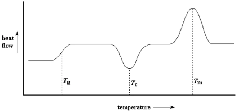
Figure 11: Example of a DSC curve of a typical semi-crystalline polymeric material ... 30

Figure 12: Typical dog-bone geometry used in a tensile test ... 31

Figure 13: Example of a stress-strain curve ... 32

Figure 14: Types of fracture of unfilled polymers ... 32

Figure 15: Difference in the tensile curves for experiment E2 ... 34

Figure 16: Typical strain rates covered by conventional load frame]. ... 35

Figure 17: Flow curve from Moplen EP3307 ... 38

Figure 18: PVT curve for Moplen EP 3307 ... 40

Figure 19: Finite element model (feeding system and part) ... 41

Figure 20: Graphic visualization of the moulding window analysis ... 43

Figure 21: Ferromatik-Milacron k85 injection moulding machine ... 46

Figure 22: Sample weight variation as a function of the holding time ... 46

Figure 23: Model mesh with the selected region for the calculation of the TMI ... 47

Figure 24: Sample for the skin ratio evaluation ... 48

Figure 25: Example of the microstructure observed by PLM ... 48

Figure 26: Schematic representation of the procedure used to obtain the skin samples. ... 49

Figure 27: Attenuation length vs 2θ ... 50

Figure 28: Diffraction plot of a PP sample from 45 to 58º ... 51

Figure 30: Setup for the quasi-static tensile tests ... 52

Figure 31: Frame 3941 (before fracture) ... 53

Figure 32: Frame 3942 (after fracture) ... 53

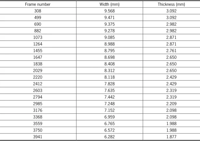
Figure 33: Correlation between area and time ... 54

Figure 34: Initial portion of the representative curve of experiment E2 ... 54

Figure 35: Deformation of the specimen during the tensile test at 20mm/min ... 55

Figure 36: Grip system ... 56

Figure 37: ISO 8256 type 3 ... 56

Figure 38: ISO 8256 type 3 modified ... 56

Figure 39: Setup for high speed tensile tests ... 57

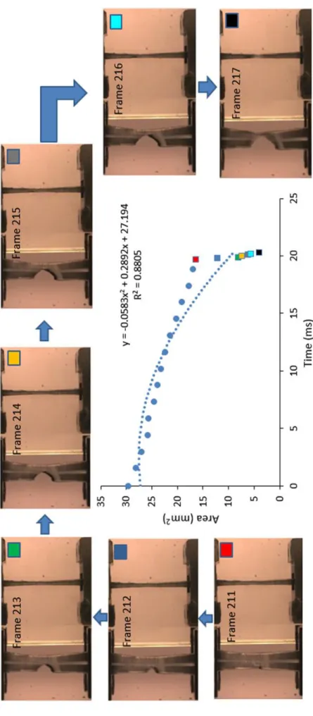
Figure 40: Frame 217 of experiment E2 at 1m/s ... 58

Figure 41: Frame 218 of experiment E2 at 1m/s ... 58

Figure 42: Variation of the area for experiment E2 at 1m/s ... 58

Figure 43: Area fitting using a 3rd order polynomial equation ... 59

Figure 44: Final area fitting for experiment E2 ... 59

Figure 45: Sequence representing the fracture of the specimen in a high speed tensile test ... 60

Figure 46:Tensile curves illustrating the correction done to the data ... 61

Figure 47: Initial part of the homogenous curve at 1m/s ... 61

Figure 48: Initial part of the homogenous curve at 3m/s ... 61

Figure 49: Comparison between the true stress curve and the engineering tensile curve at 1m/s ... 62

Figure 50: Comparison between the true stress curve and the engineering tensile curve at 3m/s ... 63

Figure 51: Effect of the processing conditions on the TMI at the end of filling ... 66

Figure 52: Relationship between the cooling index at different processing stages ... 66

Figure 53: Variation of Sa with each processing condition ... 67

Figure 54: Microstructure of E1 ... 68

Figure 55: Microstructure of E8 ... 68

Figure 56: Effect of the processing conditions on the skin ratio ... 68

Figure 57: Variation of the skin orientation and crystallinity index with each processing condition ... 69

Figure 58: The effect of the processing conditions on the skin orientation and crystallinity ... 71

Figure 59: Variation of the β-phase content with each processing condition ... 71

Figure 60: Effect of the processing conditions on the β-phase content ... 71

Figure 62: Representative DSC thermogram of each experiment within the DOE ... 73

Figure 63: Variation of σy, E and εb for all experiments ... 76

Figure 64: Tensile curves of all experiments in quasi-static tensile tests ... 77

Figure 65: Tensile curves of all experiments in high speed tensile tests (1m/s) ... 77

Figure 66: Tensile curves of all experiments in high speed tensile tests (3 m/s) ... 77

Figure 67: Effect of the main processing variables on the quasi-static tensile properties ... 78

Figure 68: Interaction influencing εb at 20 mm/min ... 78

Figure 69: Effect of the main processing variables on the tensile properties measured at 1m/s ... 79

Figure 70: Interactions influencing E and εb at 1m/s ... 79

Figure 71: Effect of the main processing variables on the tensile properties measured at 3m/s ... 79

Figure 72: Interactions influencing σy and εb at 3 m/s ... 79

Figure 73: Relationship between the thermal-stress index and the skin orientation ... 81

Figure 74: Relationship between the cooling index and the bulk crystallinity ... 81

Figure 75: Relationship between the TMI and Sa ... 81

Figure 76: Relationship between the TMV and Sa ... 81

Figure 77: Relationship between the TMI and Ωs ... 82

Figure 78: Relationship between the TMV and Ωx ... 82

Figure 79: Relationship between the TMI and χskin ... 83

Figure 80: Relationship between the TMV and χskin ... 83

Figure 81: Relationship between the TMI and k- value ... 83

Figure 82: Relationship between the TMV and k- value ... 83

Figure 83: Relationship between the TMI and χ bulk ... 84

Figure 84: Relationship between the TMV and χ bulk ... 84

Figure 85: Variation of the skin ratio with each processing condition and comparison with reference .. 88

Figure 86: Relationship between the TMV and Sa for the case study’s DOE plan ... 88

Figure 87: Relationship between the TMV and Sa for all case study's experiments ... 88

Figure 88: Relationship between the TMI and Sa for the case study’s DOE plan ... 89

Figure 89: Relationship between the TMI and Sa for all case study's experiments ... 89

Figure 90: Variation of FP with each processing condition ... 91

Figure 91: Variation of Ub with each processing condition ... 91

Figure 92:Relationship between the TMI and FP ... 91

I

NDEX OF

T

ABLES

Table 1: Electromagnetic Spectrum... 24

Table 2: Subareas of scattering as a function of the sample-to-detector distance ... 25

Table 3: Crystal systems and types of lattices ... 26

Table 4: Diffraction angle, θ, and the corresponding Miller indices and crystal form ... 28

Table 5: Properties from the data sheet of PP Hostacom EP3307 ... 37

Table 6: Cross-WLF model coefficients ... 39

Table 7: Moulding window analysis conditions: Preferable region ... 42

Table 8: Results from the moulding window analysis ... 42

Table 9: Design of experiments plan ... 45

Table 10: Measurements of the width and thickness variation in experiment E2 ... 54

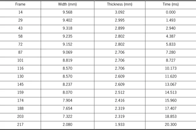
Table 11: Variation of the width and thickness for experiment E2 at 1 m/s ... 59

Table 12: Results of the thermomechanical indices ... 65

Table 13: Effect of the processing conditions on the thermomechanical indices ... 67

Table 14: ANOVA of Sa ... 69

Table 15: ANOVA of Ωs and χskin ... 70

Table 16: ANOVA of the β-phase content ... 72

Table 17: Results of σy , E and εb results for all strain rates ... 75

Table 18: Comparison between TMI ... 80

Table 19: Resume of the effect of the thermomechanical indices on the morphological parameters ... 84

Table 20: Comparison between weighted and non-weighted thermomechanical indices ... 85

Table 21: Case study DOE plan ... 87

Table 22: Results of Sa prediction resorting to thermomechanical variables ... 89

Table 23: Results of Sa prediction using TMI ... 90

Table 24: Results of the prediction of Fp and Ub using TMI ... 92

A

BBREVIATIONS

IM Injection moulding

CAE Computer aided engineering CAD Computed aided design DOE Design of Experiments AMI Autodesk Moldflow Insight PP Polypropylene

hPP Polypropylene homopolymer cPP Polypropylene copolymer iPP Isotactic polypropylene PLM Polarised light microscopy SAXS Small angle X-ray scattering WAXS Wide angle X-ray scattering NA Nucleating agent

CI Cooling index TSI Thermo-stress index TMI Thermomechanical index TMV Thermomechanical variables FLF Frozen layer fraction

MWA Moulding window analysis

N

OMENCLATURE

ε̇ Strain-rate

τw Shear stress at wall

T_b Bulk temperature

T_C Crystallization temperature T_w Mould temperature

T_i Injection temperature

T_int Temperature at the mould-polymer interface v_i Injection velocity

H Thickness of the part γ Bulk shear-rate

R Sample-to-detector distance T_g Glass transition temperature T_m Melt temperature

Sa Skin Ratio Ωs Skin Orientation k- value β- phase content

χ_bulk Bulk degree of crystallinity χ_skin Skin crystallinity index t_i Injection time Ph Holding Pressure t_Ph Holding time R2 Regression coefficient σy Yield Stress εb Strain at Break

Y_C Cooling index at the end of the filling stage τY Thermo-stress index at the end of the filling stage

1. I

NTRODUCTION

Plastic materials have a wide range of properties and their application has been introduced in several sectors from packing to aerospace, substituting in some cases, ceramics and metals. The worldwide production of these materials has been raising throughout the last decades. In 2013, Europe consumed approximately 46.3 Million tons of these materials and the automotive industry 8.5%, from which polypropylene (PP) was the most consumed polymer [1]. Polypropylene is a widely used semi-crystalline polymer that has been extensively investigated for academic and industrial purposes. This polyolefin presents a wide range of mechanical properties which are dependent, among other aspects, upon the processing technique.

Injection moulding (IM) is one, is not the most, used processing technique in the automotive industry. It offers a great flexibility in the design of parts, high production rates and high dimensional accuracy.

It is known that a layered up structure, composed of a skin and a core region, is developed when injection moulding semi-crystalline polymers. Fujiyama [2] demonstrated that the properties of the skin layer in an injection moulded PP had quite a distinct behaviour from the core layer. Nowadays, the engineering procedure to study the mechanical behaviour of injection moulded semi-crystalline polymers has been based on the scale features of this skin-core laminate arrangement. Also, because of the strong stress and temperature gradients existent in the IM process several types of hierarchical superstructures, such as the skin ratio [3]–[6], molecular orientation [7]–[10], and polymorphic crystalline structures [5], [10]–[14] are developed when processing polypropylene. Furthermore, the relationship between operating variables vs microstructural development, operating variables vs mechanical responses and morphology vs mechanical properties is not strictly straightforward [2], [15]–[22].

In an industrial context, more specifically in the automotive industry, cars are designed to be crashworthy so their components have to subjected to mechanical tests to ensure the safety of passengers and to more accurately design parts in order to save raw-material and the overall cost. One of the most extensively used mechanical tests used to obtain basic mechanical properties (e.g., elastic modulus, yield stress and strain at break) is the tensile test. Extensive knowledge is available about the mechanical behaviour of PP at quasi-static conditions (strain-rate <10-2 s-1_{) whilst due to the complicated}

experimental procedure and data interpretation not enough reliable material data has so far been determined at high strain-rates [23]–[28].

Despite all the anisotropic behaviour displayed by semi-crystalline polymers some models exist to predict the mechanical behaviour or a certain response of these materials [10], [24], [26], [29]–[31]. However, the majority of the models require the use of extensive microstructural analysis techniques which is not a cost-effective approach and therefore not applicable within the automotive industry. Thus, establishing straightforward relationships between processing conditions and the mechanical behaviour at the product development stage, enabling the prediction of properties, seems to be a valuable tool [32]. This work is divided into four sections. Firstly, identifying the most important processing variables and assess their influence on the morphological development in a lateral gated disc geometry. Secondly, study the effect of these variables on the tensile properties measured at both quasi-static and high speed conditions. Thirdly, use the thermomechanical indices (TMI) methodology , previously proposed [10], [28], [31]–[35], to correlate the morphological and mechanical responses of an automotive grade polypropylene with the thermomechanical environment developed during the injection moulding process. Lastly, an industrial-like case study will be carried out in some supplied samples to evaluate the experiments that present the highest values of peak force and puncture energy obtained through a falling weight impact test and subsequently use TMI methodology to define predictive models for these parameters.

The document is organised as follows: The chapter bellow (1.1) describes the state of the art with a specific focus on the goals of this project. The ones up to chapter 7 theoretical concepts of the experimental techniques used in accordance to what was found in literature are addressed. Chapter 7 and 8 describe the experimental procedure and the discussion of the obtained results. Chapter 9 covers the case study and finally, chapter 10 the conclusions of this work.

1.1 State of the Art

1.1.1 Structure development during the Injection Moulding (IM) process

Regarding the skin ratio, authors such as Fujiyama and Azuma [3] studied the effect of the melt temperature on the skin layer of several isotactic polypropylenes, both copolymer (cPP) and homopolymer (hPP). As a conclusion of their work they observed through polarised light microscopy (PLM) that with the decrease of this operative variable the skin layer increased. Housmans et al. [4] used capillary rheometer to drive several melted isotactic polypropylenes into a simple rectangular mould using different piston velocities. Though PLM they were able to identify 4 different layers from the edge to the core of the

sample, a skin layer, a transitional layer, a shear layer and an isotropic core. The authors noticed that when lowering the injection velocity both the transition layer and shear layer increased. Shen et al .[5] evaluated the skin thickness developed in and injection moulded iPP rectangle along the flow direction. The results showed that the skin layer diminishes along the flow path and that with different moulding temperatures, at the same distance from the gate, the lower the melt temperature the thicker the layer. Viana [6] injection moulded cPP parts with different geometries and explored the processing conditions affecting the development of the skin layer in the IM process. He noticed that three processing variables had influence on this parameter. The melt temperature, mould temperature and the injection velocity (flow rate). The first had a strong effect on skin layer and the author justified this by indicating that the raising in the melt temperature resulted in a larger time to reach the crystallization temperature and relaxation time, both effects contributing for the skin thinning mechanisms.The mould temperature had a low contribution for the development of this parameter and showed an opposing effect. A decrease of this operative variable raised the cooling rate, which reduced the time to reach to the crystallization temperature resulting in a thicker skin. However it also decreased the crystallization temperature by increasing the time to reach this thermal transition, thus leading to thinner skin. Lastly, the injection flow rate. The author stated that an increase of this parameter raised the temperature and shearing level of the melt. The latter phenomena has two different effects: it increases the crystallization temperature therefore reducing the time to reach the crystallization temperature (thinner skin); and it decreases the material relaxation time (thinner skins).

As for the molecular orientation and crystallinity developed when processing PP, due to the complex combination of the imposed stress field and cooling rate which strongly affects the crystallization kinetics, the macromolecular chains in the melt are highly extended forming supermolecular structures with central bundles (shishes) in which radial lamellae grow epitaxially (kebabs) [36]. Varga and Karger [11] studied the shear-induced crystallization of isotactic polypropylene (iPP) homo-, block, and random copolymers. In their study, it was evidenced that melt-shearing caused by fibber pulling was associated with the development of α-row-nuclei which served as self-nuclei of the bulk crystallization process and could induce the growth of the β-modification resulting in a polymorphous composition. Tribout et al. [12] observed the effect of shear in the crystallization kinetics of an Impact polypropylene copolymer and concluded that the nucleation density was strongly enhanced by this parameter. Faravo et al.[7] evaluated the molecular orientation by WAXS in the skin layer of an injection moulded iPP, both nucleated and non-nucleated. As a conclusion of their work, they showed that the most influential processing parameters were the mould temperature and flow rate. They observed that as the mould temperature increased the

characteristic molecular orientation of PP decreased due to the decrease of the cooling rate and the increase of the relaxation time, and, as the injection flow rate increased, an increase of the distinctive molecular orientation of PP was observed due to the increase of the flow velocity. Mendonza et al. [8] studied the molecular orientation in injection moulded plates with 1 and 3 mm of thickness using a commercial PP homopolymer (hPP) and resorting to infrared dichroism and WAXS. The authors varied the mould temperature (from 20 to 40 ºC) and injection time (1.6 to 0.7s). They noticed that, paradoxically, the increment in injection velocity had no large influence when tripling the thickness of the moulding. They concluded that the thickness of the part is the factor which governed the global level of crystalline orientation. Van Erp et al., [9] studied the effect of the injection velocity in thin walled rectangular plates. They concluded that a lower injection velocity resulted in a higher degree of orientation in the flow direction. Cermak et al. [13] evaluated the effect of the mould temperature and hold pressure in the variation of crystallinity in the skin layer by WAXS for both α and β iPP. They noticed an increase of χ_skin for a raise in the mould temperature and a decrease in hold pressure. Demiray et al. [37] obtained a rather uniform crystallinity profile through the sample thickness of iPP mouldings. They justified this by reporting limitations on the experimental procedure and by stating that secondary crystallization occurred during the sample storage. Also, the crystallinity profile was not affected by the injection velocity, mould temperature and hold pressure, possibly due to the high crystallization rates of the used PP. Viana et al. [10] studied the effect of processing conditions (v_i, T_i and T_w) on some morphological parameters, through the use of thermomechanical indices, namely the skin orientation and crystallinity index measured by WAXS. The authors noticed that the shear stress played an important role in Ωs. An increase in this parameter led to a higher value of orientation. Regarding χ_skin, they noticed that a higher shear and thermal level led to an increase of the degree of crystallinity in the skin layer.

Concerning the β-phase content, Shen et al.[5] studied the development of β-crystals along the flow direction of an injection moulded rectangular part as a function of the melt temperature. They observed that this parameter diminished with the distance from the gate. Cermák et al. [13] evaluated the effect of the mould temperature and hold pressure on the structure of isotactic polypropylene (iPP), both α-iPP and β-nucleated (β-iPP), namely the skin layer thickness, crystallinity and β-phase content. To assess the crystallinity and β-phase content they used WAXS and concluded that a raise in the mould temperature led a positive effect on the crystallinity and β-phase content in the specimens, particularly in the skin region. On the other hand, when rising the hold pressure a negative influence on the crystallinity and β-form content was manifested throughout the bulk of both α and β- iPP specimens. He also stated that

of β-iPP over α-iPP can be attributed to a combined effect of the following factors (sectors): the α to β phase transformation induced by mechanical load, the enhanced mechanical damping of β-iPP or the peculiar lamellar morphology of β-iPP. Zhang et al. [14] studied the structural evolution of a β-nucleated iPP in a tensile test by in-situ WAXS. They compression moulded plates and took tensile specimens to perform tests at various temperatures (30, 60, 90 and 120ºC). They observed that a β-mesophase transition occurred for the lowest test temperature while for the remaining test temperatures a β-α transition took place.

1.1.2 Mechanical properties of IM parts

Fujiyama [2], demonstrated that the mechanical properties of the skin layer in an injection moulded PP have a quite distinct behaviour from the core layer. The first presented a more brittle behaviour and a latter a more ductile one.

Roman et al.[15] studied the effect of the mould temperature and hold pressure on the tensile properties of α and β-nucleated polypropylene. They observed a positive effect of higher values of mould temperatures on the elastic modulus and a negligible effect of the holding pressure. Also, none of the previous processing variables showed any significant effect on the yield stress. Regarding the strain at break, since β- spherulites have a more ductile behaviour, the nucleated conditions displayed a higher deformation value. Zhou and Mallick [38] assessed the effect of the melt temperature and hold pressure on the tensile properties of a talc filled polypropylene. They noticed that in the flow direction the yield stress increase with increasing hold pressure but were relatively insensitive to the melt temperature.

Barbosa et al. [32] evaluated the effect of the processing conditions on a talc filled PP in a falling weight impact test. They concluded that the most significant processing variables were the injection and mould temperature. A decrease of these variables led to an increase of the peak force, peak energy and puncture energy.

Kalay and Bevis [16] reported that in conventional injection moulding, a very high injection speed can result in the decrease of the modulus due to shear heating. However, for low values of this operating variable a decrease in the modulus can also be obtained due to low molecular orientation. As for the injected temperature, they referred that a low value of this variable could lead to a decrease in the modulus due to the occurrence of the β-phase. Regarding the holding pressure, they referred that higher stiffness values could be obtained due to the promotion of molecular orientation.

Viana et al.[17] studied the effect of the skin thickness on the tensile properties of a PP copolymer. They observed that yield stress and modulus increased with the increase of the skin layer while the strain at break decrease with this parameter.

Van der Wal et al. [18] studied the effect of crystallinity on the fracture of polypropylene. They reported that modulus and yield stress increased almost linearly with increasing crystallinity. Parenteau et al. [19] studied the effect of crystallinity on the elastic properties in injection moulded polypropylene. They reported that an increase in crystallinity and in the mean thickness of the crystalline lamellae resulted in a higher elastic modulus. Tordjeman et al. [20] assessed the effect of different crystalline structures (α and β) on the mechanical properties of PP. They added different amounts of β-nucleating agent to an iPP and then compression moulded plates in order to produce tensile specimens. They observed that the yield stress and modulus decreased with the increase of the β-phase content and that the strain at break increased with the β-content.

Viana [21] injection moulded cPP with different processing conditions and evaluated the yield stress at several test velocities (2, 10, 100, 500 mm/min and 3 m/s). He reported that the yield stress increases with the thickness and level of the crystalline phase orientation of the skin layer and the thickness of the core lamella. He also mentioned that, as the strain-rate increased the contribution of the morphological parameters such as the skin layer saturated and the effect of the core layer became more pronounced. Way et al.[39] studied the effect the spherulite size (R_s) on the yield stress. They observed that as R_s increased, up to a spherulite radius of 100 µm, the yield stress also increased. R_s with higher values led to the decreased of this mechanical property.

Kalay and Bevis [22] evaluated the effect of molecular orientation on the mechanical properties of PP produced by conventional and shear-controlled orientation injection moulding. They remarked that the thickness of the moulding is critical in achieving high molecular orientation and that the pronounced orientation obtained from SCORIM increased the Young’s modulus.

There are not many studies regarding high speed tensile tests of polymeric materials [24]–[28] mainly because no standard procedure exist. This makes the experimental procedure and data interpretation hard to evaluate. Only a recommendation procedure by the Society of Automotive Engineers (SAE) exists. Zrida et al [24] and Schoßig [26] studied the effect of the strain-rate in a tensile test on a polypropylene. They both found that the tensile strength increased with an increase of the strain-rate. Raisch and Moginger [25] used a new approach to calculate the elastic modulus and showed that the strain-rate dependency of the modulus could be used to get rid of the stress oscillations superimposed on the stress

signal. Xiao [27] evaluated the procedure proposed by the SAE guideline and concluded that the generated results could be ranked as good when using the criteria provided by the guideline.

1.1.3 Modelling the mechanical behaviour of IM parts

Up to this point it is obvious the final performance of a part is highly dependent upon the morphological development and strain-rate. To simulate the mechanical behaviour of polymer materials it is necessary to draw up a model which accounts for the response of the polymer to various mechanical loads, as well as their strain-rate dependency. Several models to predict mechanical properties in polymeric structures exist, and they can be classified into three categories: phenomenological [24], [26], [29], empirical [10] and micro-mechanical [30], [31]. In the case of the micro-mechanical, the crystalline structures are treated as reinforcements in the amorphous phase [30] or in the case of the laminate theory, the thickness of the sample is discretised into layers. Each layer assumed to be made of an homogeneous isotropic material having a constant level of crystallinity and spherulite size [31]. The phenomenological models like the Hyper-Visco-Hysteresis (HVH) model [24], [29] predicts the strain-rate behaviour based on a rheological model accounting the hyperelastic, viscous and hysteresis contributions of the material. The G’Sell-Jonas model [26] comprises the viscoelasticity, viscoplasticity, strain hardening and the influence of temperature. However, the majority of the above mentioned models does not correlate the processing conditions and subsequent morphological structure with the mechanical properties.

The thermomechanical indices (TMI) methodology was pioneered by J.Viana [33] and dates from the late 90’s. It aims to correlate physical phenomena involved in the injection moulding process with the morphological and mechanical development in a part. The author derived two thermomechanical indices referent to the filling stage: the thermo-stress index (τY) and the cooling index (Yc). The first intends to

indirectly quantify the orientation imposed during the mould filling, and the latter to indirectly quantify the crystallinity level in the core. In his doctoral thesis [33] he found that the same morphological parameter in different geometries, therefore leading to a different thermomechanical environment, had a different trend on the TMIs. To be more specific, he studied the effect of τY and Yc on the skin ratio for a dumbbell

and disc specimen. In the dumbbell specimen the skin ratio increased with a raise in τY whereas for the

disc geometry the skin layer increase with the decrease of τY. He further studied the relationship between

the thermomechanical indices in dumbbell specimens with other morphological properties such as the skin orientation, β-phase content and skin and core crystallinity [10], [28], [31], [34], [35].

Cunha et al. [34] gave another contribution to this methodology by proposing a method to weight the TMIs with the skin ratio. They obtained a substantial improvement in the regression coefficients between the TMI and tensile properties (yield stress, elastic modulus and strain at break). Using this method Viana et al.[28] established relationships between the TMIs and tensile properties measured at low (2mm/min) and high speed (3m/s) tensile tests. For the quasi-static conditions they observed that all tensile properties increased with the increase of both weighted indices and that for the high speed tests the modulus and yield stress increased with the increment of both weighted indices and the strain at break decreased with the increment of the TMIs.

In more recent years, Barbosa et al. [32] tried to further develop this methodology in order to encompass the packing and cooling stages of the injection moulding cycle. They derived new indices and tried to predict the impact response, namely the peak force (F_P), peak energy (U_P) and energy at break (U_b), of an injection moulded talc-filled polypropylene through a falling weight impact test. They obtained good results, being the biggest deviations for predicted vs measured results of 7% for F_P and 23% for U_p and U_b. Despite the good results, and as final remark, they stated that the TMI methodology and the mechanical properties predictive tool was still under refinement.

1.2 Goals

The scope of this work is to characterise the morphological and mechanical properties evaluated through polarised light microscopy, differential scanning calorimetry, wide angle x-ray diffraction, quasi-static and high speed tensile tests of an automotive grade thermoplastic (Hostacom EP 3307) as a function of the processing conditions and to subsequently establish predictive models to correlate mechanical responses with the thermomechanical environment developed during the injection moulding process.

The specific goals are:

1. Identify and quantify the effect of processing conditions that mainly influence the skin ratio, molecular orientation, crystallinity, β-phase content and some mechanical properties (yield stress, modulus and strain at break) using a lateral gated disc geometry;

2. Characterise the thermomechanical environment of different processing conditions with an injection moulding simulation software, namely Autodesk Moldflow Insight 2012;

3. Correlate the obtained results from the morphological and mechanical characterisation with the thermomechanical indices methodology;

4. Evaluate the performance of some supplied lateral injected discs in a falling weight impact test and establish a model to predict the peak force and puncture energy (case study).

2. I

NJECTION MOULDING

2.1 Technology

There are several processes to mould plastic materials (e.g., extrusion, rotational moulding, thermoforming, blow moulding, calendaring), but only injection moulding allows for a great flexibility in the design of complex parts as well as great production rates and high dimensional accuracy.

The injection moulding process had a great technological expansion by the time of the Second World War, when the petrochemical industry enabled the sale of a set of thermoplastics at competitive prices. After the second half of the 1950’s the process has been subjected to several technological improvements, becoming one of the most widely used technologies to this day [40], [41].

Injection moulding consists of a repetitive process in which melted (plasticized) plastic is forced (injected) into a mould where it is held under pressure until it is solidified and removed, replicating the geometry of the cavity. A feeding system conveys the melt from the machine cylinder to the mould cavity(ies). It may consist in a single or multiple cavities of similar or dissimilar shape. The process ends with the opening of the mould and subsequent extraction of the part(s).

A conventional injection moulding machine is typically composed of four units (Figure 1): a) Power unit - responsible for providing energy to the various machine actuators;

b) Injection unit - promotes the transport, heating, plasticizing and homogenization of material from the bottom of the hopper to the injection nozzle. It also ensures injection and pressurization of the melt;

c) Clamp unit - allows the setting and movement of the mould. This is responsible for keeping the mould closed during the injection and pressurization phases. It also integrates the devices required for the extraction of parts;

d) Control unit - integrates the devices necessary to ensure the monitoring and control of various process variables. It is the operator interface and communication with peripherals or information management systems.

Figure 1: Conventional injection moulding machine

2.2 The Cycle

The injection cycle (Figure 2) can the defined as the set of operations that are carried out in the injection moulding machine during the production of consecutive parts. This process includes the following steps:

1. Mould closing – this is the operation that starts the cycle and should be as fast as possible, taking into account that the contact between the two parts of the mould should be smooth in order to prevent any damage to the surface;

2. Injection - at this stage, and after melting/softening, the polymeric material is forced to flow into the cavity;

3. Holding (Pressurization) - after the filling stage it is necessary to continue and pressurize the moulding in order to prevent reflux and contraction of the material;

4. Cooling - when the melt comes into contact with the mould, it loses heat in the form of conduction to the metal of the mould cavity. This phase is concluded when the temperature of the material decreases to the point of being able to remove the part from the cavity without distortion of the product.

5. Extraction of the part – The time needed to fulfil this operation is a function of the machine, namely the characteristics of the clamping unit and dislocation of the mould during the opening time;

Figure 2: The injection moulding cycle [42]

The objective of the process, at an industrial level, is to minimize the time of each operation and ensure that the parts leave with the specified specifications. The optimization of this cycle basically ensures economic competition given that the initial investment for the acquisition and installation of the IM equipment, as well as the manufacturing of moulds, are quite high.

To reduce the time needed for the optimization of the IM process and to establish better processing conditions, computer aided engineering (CAE) and computer aided design (CAD) tools have been widely implemented. These techniques employ software to design and simulate the performance of a component in order to improve product designs or assist in the resolution of engineering problems. A software like Autodesk Moldflow Insight (AMI) is a good example of the CAE/CAD implementation. It has been used by several authors to improve the injection mould design and plastic part design, as well as the injection moulding process [43]–[46].

2.3 Thermomechanical Environment

In the injection moulding process, the thermal and mechanical phenomena are strongly coupled because of the dependence of the viscosity on the shear rate and temperature. The complex thermomechanical environment imposed to the melt results, mainly, from the combined effect of:

 the high shear rates associated to the flow rate;

 the moulding geometry;

 the material rheological properties;

 high cooling rates resulting from the relatively low temperatures of the mould walls;

 pressure level of the holding stage;

These thermomechanical conditions affect the morphological development of a polymeric part, thus determining its final mechanical properties (and others).

During the injection (filling) stage, the melt is driven through the feeding system into the mould cavity(ies). Due to the flow fountain effect and the high values of shearing, the macromolecules are stretched and frozen almost immediately forming a skin layer. The next portion of melted polymer flows rapidly in the central regions of the moulding, now thermally insulated by the previously formed solidified skin. The macromolecules relax over the available period of time or in the case of semi-crystalline polymers, until the crystallization temperature is reached. The relaxation phenomenon depends on the structure of the polymer, the cooling rate and pressure. During the next stage (holding), the melt velocity is drastically reduced, but a small amount is still introduced in the mould cavity to compensate for the volumetric shrinkage. This additional input of material will influence the shear stress distribution especially near the solid/melt interface due to the lower local temperatures and hence higher viscosity of the melt. Meanwhile, the core cools down under a relatively high pressure. The duration of this step is usually determined by the time need to reach the solidification of the gate. The solidified layers act as insulators during the cooling due to the low thermal diffusivity of the polymer allowing slower cooling of the core under a gradual reduction of the local pressure [28], [34].

3. T

HERMOMECHANICAL

I

NDICES

The mechanical properties of polymers, especially semi-crystalline ones, are highly dependent upon the morphological development and cannot be related to one single factor. The establishment of quantitative relationships between processing, morphology and mechanical properties in injection moulding remains an open issue, which creates the need for developing engineering methodologies that, even with empirical and phenomenological approaches, can handle this reality. In 2013 [32], [47] a methodology was developed to predict local mechanical properties of injection moulded parts based on several thermomechanical variables (TMV) obtained from Autodesk Moldflow Insight in a filling, packing and cooling simulations and the TMI. A software was developed which consisted in importing relevant results from the computer flow simulations and, accordingly, predict the mechanical properties of a 2.5D finite-element model mesh (triangular elements on surface of the model). The application computes the mechanical properties (per element of a dual domain mesh) based on the TMI equations and a set of regression equations resulting from both simulations and experimental analysis. The user only imports the TMV into a root directory, grouping them into three distinct modules:

 Geometrical definition of the component;

 Set of processing conditions, including material-specific properties;

 TMV for all the time instants of the injection moulding process. The thermomechanical variables are:

The bulk temperature (T_b), which is a weighted average temperature across the thickness of the moulding. The temperature of polymer melt changes not only with time and location but also with the thickness during the entire injection moulding cycle. It represents the energy that is transported through a particular location and is defined by equation 1.

𝑇̅̅̅ = 𝑇̅ +𝑏 1 ℎ ∫ (𝑇(𝑧) − 𝑇̅)𝑣(𝑧)𝑑𝑧 ℎ 0 ∫ 𝑣(𝑧)𝑑𝑧₀ℎ (1)

Where, T̅_b is the bulk temperature, T̅ the average temperature, h the thickness of the part, v (z) the local velocity (through the thickness) and T (z) the temperature profile in the thickness direction.

The shear stress at wall (τw), which is the shear force at the frozen/molten interface, per unit area,

of the degree of molecular orientation since a higher shear stress would induce higher orientation, especially near the surface of the part.

The bulk shear rate (γ̇). This parameter is derived from the shear stress at wall, the representative viscosity (η_rep) and thickness of the part, calculated from the fluidity (S), equation 2. It is a measure of how quickly the layers of plastic are sliding past each other. If this happens too fast, the polymer chains break and the material degrades. In contrast to the bulk temperature, the bulk shear rate is not an average or weighted average of the shear rate because it can vary widely across the part thickness.

𝑆 = 𝐻

3

3𝜂_𝑟𝑒𝑝; 𝛾̇ = 𝜏𝑤

𝜂_𝑟𝑒𝑝 (2)

Finally, the frozen layer fraction (FLF). It is not strictly a TMV but rather the result of the relationship between TMV. It presents a value varying between 0 and 1 and resents the fraction of the frozen layer thickness during the IM cycle. This parameter establishes a relationship between the temperature calculated in the finite element model at each given time with a transition temperature, which in case of semi-crystalline polymers is the crystallization temperature. The polymer is considered to be frozen when the temperature falls below the transition temperature.

Viana et al. [35] first introduced the derivation of two TMI. The cooling index(Y), CI, equation 3, which characterises the thermal level of the moulding and is defined as the ratio between the superheating degree and the cooling difference. It indirectly quantifies the crystallinity level of the core. Lastly, the thermal-stress index (τY),TSI, equation 4, defined as the ratio between the level of molecular orientation

imposed during the mould filling (indirectly assessed by the shear stress at the solid/liquid polymer interface, τw) and the level of molecular relaxation occurring during cooling (assumed proportional to the

CI). Both TMI were derived for the end of the filling stage in 1997, and then, in 2000 to 2002 suffered some modifications [34], [35]. 𝑌_𝑐 = 𝑇𝑏− 𝑇𝑐 𝑇_𝑏− 𝑇_𝑖𝑛𝑡 (3) 𝜏𝑌 = 𝜏_𝑤 𝑒𝑌 (4)

Where T_c is the crystallization temperature; T_int, the temperature at the mould-polymer interface (equation 5), defined as an average temperature of the polymer (script_-m) and mould (script_-w) weighted by their

𝑇_𝑖𝑛𝑡 = 𝑏𝑤𝑇𝑤+ 𝑏𝑚𝑇𝑏

𝑏_𝑤 + 𝑏_𝑚 (5)

𝑏 = √𝜌𝐾𝐶𝑝 (6)

ρ is the density, K the thermal conductivity and Cp the heat capacity,

In more recent years, the TMIs have been subjected to improvements. Barbosa et al. [47], [48] proposed equations for the packing and cooling stages. In their report [47] the CI at the end of packing and cooling was calculated as a weighted average by the relative duration of each phase, equations 7 and 8. 𝑌_𝑐𝑓𝑝= 𝑌𝑐 𝑓 𝑡𝑓+ |𝑌_𝑐𝑝|𝑡𝑝 𝑡𝑓_{+ 𝑡}𝑝 (7) 𝑌_𝑐𝑓𝑝𝑐 =𝑌𝑐 𝑓 𝑡𝑓_{+ |𝑌} 𝑐 𝑝 |𝑡𝑝_{+ |𝑌} 𝑐𝑐|𝑡𝑐 𝑡𝑓_{+ 𝑡}𝑝_{+ 𝑡}𝑐 (8)

Ycf, Ycp Ycc, and tf, tp, and tC are the filling, packing and cooling indices and durations, respectively. The

packing time is defined at the element level and its value taken from the instant right before the pressure drops to 0. The cooling time was defined as the time needed for the FLF to be equal to 1.

The calculation of the cooling index exclusively for an individual phase can done resorting to equation 3 and substituting T_b, T_int, and T_c for their respective value at the end of each phase. T_c can be estimated by equation 9.

𝑇𝑐 = 𝑇𝑐∗+ 𝑏6𝑃 (9)

Where T_c* is the crystallization temperature at ambient pressure (assumed constant), b₆ a constant and P the maximum pressure at the end of the filling, packing or cooling stages.

The calculation of shear stress at the end of the packing and cooling stages was done analogously to the CI, where a weighted average was calculated, equations 10 and 11.

𝜏_𝑤𝑓𝑝=𝜏𝑤

𝑓

× 𝐹𝐿𝐹𝑓+ 𝜏𝑤𝑝(𝐹𝐿𝐹𝑝− 𝐹𝐿𝐹𝑓)

𝐹𝐿𝐹𝑝 (10)

The calculation of the TSI at the end of each respective phase can be done by applying equation 4 and substituting the shear stress at wall and the CI by their respective values.

A computational flow chart of this methodology is illustrated in Figure 3.

4. M

ATERIAL

Polypropylene (PP) was first produced by Guilio Natta, following the work of Karl Ziegler, by the polymerization of propylene monomers (Figure 4) in 1954 [49].

Figure 4: Polypropylene monomer

This semi-crystalline material can be divided into two different categories: homopolymer (hPP) and copolymer (cPP). The first consists of molecular chains with repeating units of polypropylene monomer. This monomer can be obtained from several different sources being the most common the steam cracking process using naphtha. The copolymer is obtain by mixing PP monomer at the first stages of polymerization with ethylene or with another comonomer such as butane [50]. An important subtype of cPP, which is used in several automotive applications, is the impact-resistant polypropylene copolymer (IPC). This polymer is prepared by a two-step polymerization: bulk polymerization of propylene and then a gas-phase copolymerization of ethylene and propylene [51]. Several authors identified 3 types of composition in IPC, ethylene-propylene random copolymer (EPR), ethylene- propylene block copolymers and propylene homopolymer [51].

Polypropylene has an asymmetric carbon and can be found in three types of spatial configuration. If the methyl groups (CH₃) are on the same side of the polymer chain, the resulting product is referred to as isotactic PP. If the methyl groups are placed in an alternating position along the polymer backbone the result is a syndiotactic PP, and, if they are displaced in a random way the result is the atactic form (Figure 5).

Polypropylene also exhibits polymorphism and may display up to four different crystal modifications: α, β, γ and a mesomorphic phase. Housmans et al. [4] cited that under standard conditions occurs the

(a) (b) (c)

formation of the α-phase with a monoclinic crystal structure characterised by the cross-hatching or lamellar branching, consisting of a daughter lamellae that grows on top of the initial (mother) lamellae. The β-phase with its trigonal unit cell is formed in the presence of a temperature gradient [52], strong imposed molecular orientation [11] or with the addition of nucleating agents [53]. The occurrence of the γ phase, with its orthorhombic unit cell, can be originated due to low stereo-regularity of the chains [54], low molecular weight [54], pronounced molecular orientation [55], and copolymerization (e.g., with ethylene) [56]. Finally the mesophase, containing a pseudo-hexagonal unit cell is formed under high cooling rates [4], [57].

5. D

ESIGN OF

E

XPERIMENTS AND

A

NALYSIS OF

V

ARIANCE

In general the design of experiments (DOE) can be defined as a rigorous, systematic method to solve engineering problems in a process/system, applying principles and statistical techniques at the data collection stage to ensure the generation of valid, defensible, reproducible, and supportable conclusions. In addition, all of this is carried out in order to ensure minimal time and monetary expenses.

A process can be defined as the transformation of inputs into outputs. In the context of manufacturing, the inputs can be regarded as materials, processing conditions, procedures, etc. and the outputs (also referred to as the responses) can be the quality or a performance characteristics of a product, Figure 6. In a process, there are variables which the user can easily vary during an experiment who have a key role in the characterisation process. On the other hand, there can also be uncontrollable variables which are responsible for variability in the system. The knowledge of these and their influence is fundamental for the strategy of robust design [58].

When performing a DOE, intentional changes in the inputs will be made in order to observe changes in the outputs. There are several DOE techniques, like the Taguchi method [32], response surface methodology [59] and central face composite [28], among others, which several authors have used in order to define and study the optimization of different parameters in the injection moulding process.

Figure 6: General model of a process/system

The use of statistical methods have a great importance in the conduct, analysis and interpretation of engineering data. The analysis of variance (ANOVA) is used to compare the variance within a data population (factors) and is usually implemented with DOE plans. This statistical procedure has been used by some authors [48], [60] to evaluate the trend and contribution of operative variables on a certain response. It is a statistical method based on the Fisher-Snedecor distribution that subdivides the total

variance within a specific set of data associated with specific sources of variation, in order to test a hypothesis (null hypothesis test) on the model’s parameters. This null hypothesis tests checks if:

 The mean of each data population (factor) is the same for all conditions;

 The mean of each data population is different for all conditions.

If the test is true, for a certain degree of confidence (α), then the factor in question does not affect the response. If the hypothesis is rejected, at least one parameter is significant for the model and it influences the response. The mathematical derivations of this statistical analysis are not mentioned in this thesis, however, they can be accessed in [61].

6. C

HARACTERISATION

T

ECHNIQUES

6.1 Polarised Light Microscopy (PLM)

There are several techniques to observe the morphology of amorphous and semi-crystalline polymers. The knowledge of the interaction between electromagnetic waves and matter is of crucial importance for the selection of the adequate technique.

The image that is sought to reproduce the microstructure of a material must be in sufficient resolution, contrast and magnification to allow a comfortable observation. Polarised light microscopy (PLM) consists of a typical microscope combined with two polarised filters perpendicular to each other, one after the objective lens (analyser) and the other before the condenser lens (polarizer).

Light is an electromagnetic wave that propagates in all directions and when it contacts the polarizer, part of it is filtered and the resulting wave only propagates in one direction. If this polarised light goes through the sample without changes in the polarization plane it will be absorbed by the analyser and, as a result, the obtained image will be completely black. This phenomenon is called the extinction position and reflects the quality of the polarizers. Most efficient polarizers are made of transparent crystals, such as calcite, but light can also be polarised by using a sheet of aligned long-chain polyvinyl alcohol molecules impregnated with aligned microcrystals of polyiodide, like the one introduced by the Polaroid Company [62].

In the characterisation of polymeric materials the use of PLM can be seen in the:

 Detection and measurement of birefringence in films and moulded parts [63];

 Observation of the crystalline morphology of semi-crystalline polymers [5], [28], [64];

 Identification of additives [65] (e.g. fillers and reinforcements);

 Observation and measurement the optical fusion and crystallization point of semi-crystalline polymers (when the microscope is incorporated with a hot plate) [66].

In literature, semi-crystalline materials who are injection moulded develop a sandwich like structure. Near the mould a crystalline structure who is highly oriented, usually referred to as the skin layer is developed and, moving away from the mould wall, the material has more time to crystalize resulting in morphological structures with different shape and dimensions (core). The dimensions of these structures are dependent upon the thermomechanical history developed during the IM cycle and result in different mechanical properties, both along the thickness and the flow direction [64].

With the images taken from PLM one can calculate the skin ratio (Sa). This parameter intends to quantify the amount of oriented material developed during the IM process.

6.2 X-Ray Diffraction (XRD)

X-Rays are a high energy type of electromagnetic radiation, table 1. They were discovered by Wilhelm Conrad Röntgen in 1895 [67] and nowadays serve in a lot of applications, ranging from medical to security procedures (e.g., tomography and airport security).

In the case of polymeric materials the use of X-ray methods are an important characterisation tool that provides important solid-state structural information ,e.g., identification of phases, degree of crystallinity, crystallite size, molecular orientation, and identification of structural parameters (e.g., the unit cell parameters) in unknown crystalline materials.

Table 1: Electromagnetic Spectrum. Adapted from [68]

Wavelength Frequency Range Wavelength (m) Frequency (Hz) Low High Gamma radiation < 10-11 > 1019

X-Ray radiation 10-9- 10-11 1017- 1019 Ultraviolet radiation 10-7- 10-9 1014- 1017 Infrared radiation 10-5- 10-7 1012_{- 10}14

Microwave radiation 10-2- 10-5 109- 1012 High Low Radio waves > 10-2 < 109

In principle, the x-ray equipment measures the flux of x-ray photons (scattered radiation) as a function of the diffraction angle (θ).

There are two main types of X-Ray scattering techniques, small angle x-ray scattering (SAXS) and wide angle x-ray scattering (WAXS). The main difference between the two is the sample-to-detector distance (R). In WAXS, short distances between sample and detector are used, usually ranging from 0.05-0.2 m and in SAXS, distances from 1-3 m [69]. There are variances (subareas) in this two techniques, e.g., middle angle x-ray scattering and ultra-small angle x-ray scattering) which result in a different type of scale resolution. Stribeck [69] displayed the subareas of x-ray scattering as a function of R, assuming the wavelength (λ) produced by Cu (0.15418 nm). The results are presented in Table 2.

Table 2: Subareas of scattering as a function of the sample-to-detector distance, [69]

Subarea R (m) Focus

WAXS 0.05 – 2 Arrangements of chain segments MAXS 0.2 – 1 Liquid-crystalline structure SAXS 1 – 3 Nanostructure 3-50 nm USAXS 6-15 Nano and microstructure 15-2000nm

There are two types of setup schemes for the scattering experiments. In symmetrical-transmission mode the radiation from a source (1) is monocromatised and collimated by the incident beam optics (2). A beam passes through the sample (3) and is decomposed into a primary and diffracted components. The primary beam (unscattered) hits a beam stop (5) and the diffracted beams the detector (4). This setup allows the change of the sample-to-detector distance enabling the use of WAXS and SAXS but requires the use of 2D detectors, Table 2 and Figure 7. In a symmetrical- reflection x-ray setup the angle θ changes while recording the intensity of the scattered radiation being measured, typically, by a linear detector [70].

Some polymers, like polypropylene, have the capability of crystallization and polymorphism which in due turn contribute for the mechanical response of the material, thus rendering important the quantification of these morphological features.

Crystals are defined as a periodic atomic or molecular array with tridimensional shape. The unit cell is the simplest repeating unit in a crystal and their periodic arrangement is called a lattice. They are defined by three axes (abc) and the angles between them (αβγ), Figure 8. In 1845, August Bravais demonstrated the existence of 14 types of lattices within 7 crystal systems. The lattices are classified as follows: simple, body centred, face centred and base centred. The crystal systems as: cubic, trigonal, monoclinic, orthorhombic, tetragonal, triclinic and hexagonal [71].

(a) (b)

Figure 7: X-ray setup a) Transmission setup; b) Reflection setup, 1-X-ray source; 2- Beam optics; 3- Sample; 4- Detector; 5- Beam stop; R- Sample-to-detector distance. Adapted from [70].

Table 3 presents a resume of the crystal systems and lattices along with the cell parameters of each system. In 1839, W.H Miller proposed a methodology to describe the facets or internal planes of a crystal structure in relation to the unit cell axes though a series of indices (h,k,l). They are characterised, among other things, by describing the angular position to the crystallographic axes but not their actual distances to the origin. Only the ratio of these indices are important, e.g., (330) (220) (110) represent the same set of planes. Also, when a plane is parallel to a coordinate system the miller index assumes the value 0 [72].

Table 3: Crystal systems and types of lattices. Adapted from [72]

Crystal System Unit Cell Characteristics Lattice Type

Simple Base Centred Body centred Face centred Cubic α = β = γ = 90º a = b = c Tetragonal α = β = γ = 90º a = b ≠ c Hexagonal α = β = 90º γ = 120º a = b ≠ c Trigonal a = b = c α = β = γ ≠ 90º Orthorhombic α = β = γ = 90º a ≠ b ≠ c Monoclinic α = γ = 90º ≠ β a ≠ b ≠ c Triclinic α ≠ β ≠ γ ≠ 90º a ≠ b ≠ c