Altitude Control of an Underwatervehicle Based on Computer Vision

Altitude control of an underwater

vehicle based on computer vision

Pedro Miguel Flores Rodrigues

MASTER’S DEGREE INELECTRICAL ANDCOMPUTERSENGINEERING Supervisor: Nuno Alexandre Cruz (FEUP)

Co-Supervisor: Andry Pinto (INESC-TEC)

A contínua necessidade de melhorar o processo de supervisionamento dos oceanos tem vindo a promover a criação e desenvolvimento de novas tecnologias focadas nesta área. Visto que as mis-sões subaquáticas, por vezes, implicam ambientes hostis e perigosos para a intervenção humana, é comum recorrer a sistemas baseados em veículos subaquáticos para a realização destas missões. No decorrer da extração de informação numa missão envolvendo veículos subaquáticos, a distân-cia entre o veículo e o fundo do mar ou outros obstáculos deve ser cautelosamente controlada para garantir a segurança do veículo e o sucesso da missão. Tipicamente, para lidar com esta tarefa, é utilizado um sistema baseado na tecnologia sonar. Embora esta solução simplifique o problema e seja eficaz na maioria dos casos, pode implicar algumas desvantagens em algumas condições subaquáticas e em alguns veículos com certas especificações.

Nesta dissertação é apresentado um sistema capaz de controlar a altitude de um veículo aquático recorrendo a visão computacional. O sistema foi dividido em 2 módulos, um módulo capaz de calcular a altitude baseado em visão computacional (Sensor module) e um módulo que para além de aplicar um filtro de Kalman às medidas, é responsável por controlar este valor (Filtering and Control module). O veículo utilizado para validar e testar os módulos criados foi um profiler desenvolvido em [1], cujo principal objetivo é a navegação vertical.

O Sensor module foi implementado baseado na utilização de 2 dispositivos lasers colocados paralelamente a uma câmara CCD. O princípio de triangulação foi usado para calcular a distância aos obstáculos. Este módulo é também capaz de devolver informação acerca da qualidade das medidas adquiridas e aplicar operações aritméticas na informação obtida. Os testes realizados mostraram um erro relativo médio igual a 1 % no intervalo de altitudes de 0 a 2.5 m.

Relativamente ao Filtering and Control module, a solução adoptada para o controlo é baseado na comutação de 2 controladores, um controlador de velocidade (baseado num controlador PI), e um controlador de posição (baseado num controlador PD). O controlador de velocidade é usado quando o veículo se encontra longe da referência de posição pretendida, e após a comutação, o controlador de posição atua de modo a completar o movimento. O modelo matemático do veículo foi obtido de modo a dimensionar os controladores. O controlador de posição foi dimensionado de modo a garantir que não haveria overshoot e que a comutação seria suave relativamente à atuação dos motores. Um método de afinação dos parâmetros do controlador de velocidade foi criado que permite o seu dimensionamento baseado no custo energético, máxima corrente, e exigências temporais. Os controladores foram validados utilizando o simulink toolbox do Matlab.

Utilizando o simulador de ambientes aquáticos UWsim, a arquitectura desenvolvida para in-tegração dos 2 módulos foi testada. Durante os testes realizados, um movimento descendente foi executado de modo a testar os controladores dimensionados, a comutação entre os controladores, a interação entre os 2 módulos, e a eficácia da fase de filtragem em casos em que erros foram in-duzidos no Sensor module. Os resultados obtidos provaram que o sistema interage corretamente, os controladores induziram uma boa transição em direção à referência de altitude, e a fase de filtragem foi capaz de lidar com os erros induzidos.

The desire of improving and developing new technologies targeting the ocean’s supervision is con-tinuously increasing. Since underwater tasks might involve hostile environments far too hazardous for human, it is typical to resort to systems based on underwater vehicles. During the extraction of information, the distance between the vehicle and the sea floor or other obstacles must be warily controlled to ensure its safety and the reliability of the missions. Commonly, to deal with this task, a system based on sonar technology is used. Although this solution simplifies the problem and is effective in most cases, it carries disadvantages in some underwater conditions and in some vehicles with certain specifications.

In this work it is presented a system capable of controlling the altitude of an underwater ve-hicle using computer vision. This system was divided into 2 modules, a module responsible for measuring the distance based on computer vision (Sensor module) and a module that applies a Kalman filter to the data and is capable of using the filtered data to control the altitude of the vehicle (Filtering and Control module). The vehicle used in order to validate and test the mod-ules created was a profiler developed in [1] which main purpose is the navigation in the vertical direction.

The Sensor module was implemented based on two laser pointer devices placed parallel to one another beside a CCD camera. In order to calculate the distance of the vehicle towards the obstacle, the laser triangulation principle was used. Furthermore, the Sensor module is capable of retrieving information about the quality of the measurements and apply mathematical operations like circular average. The tests performed showed an average relative error equal to 1 % in the range from 0 to 2.5 m.

Relative to the Filtering and Control module, the solution adopted regarding the control stands on the switching of two controllers, a velocity controller (based on a PI approach), and a position controller (based on a PD approach). The velocity controller is used when the vehicle is far away from the target position reference, after the switching point the position controller is used in order to reach the reference. The mathematical model of the vehicle dynamics was used in order to design the parameters of the controllers. The position controller was designed in order to achieve a smooth switching between the controllers and also to guarantee no overshoot. A method of designing the velocity controller was created where the parameters can be tuned based on the energetic cost, maximum current, and temporal demands that depend on the mission’s demands. The designed controllers were validated using the simulink toolbox from Matlab.

Using the UWsim underwater simulation environment the overall architecture developed inte-grating both modules was tested. During these tests a descent movement was performed testing the performance of the controllers designed, the switching of the controllers, the interaction between the 2 modules, and the effectiveness of the filtering phase in cases where errors were induced in the Sensor module. The results obtained showed that the overall system is interacting correctly, the controllers allowed a good transition response towards the position reference, and the Kalman filter was able to handle the errors induced.

Ao professor Nuno Cruz, um especial agradecimento pela exímia orientação ao longo desta dis-sertação, pelas criticas, atenção, e mais importante, pelos ensinamentos e conhecimento que me transmitiu.

Quero também agradecer ao professor Andry Pinto pela ajuda ao longo da dissertação e ao João Monteiro que se mostrou sempre disponível a esclarecer qualquer dúvida acerca do profiler ao longo deste caminho.

Não poderia deixar de agradecer a todos os meus amigos mais próximos que de uma forma directa ou indirecta, contribuíram para a elaboração deste projeto, pelo apoio e sobretudo pelos momentos de descontração que proporcionaram.

Quero também agradecer aos meus pais pelo seu apoio incondicional. Um especial agradeci-mento ao meu avô pela educação durante a minha infância que tanto contribuiu para a forma como encaro os obstáculos ao longo da minha vida.

Pedro Rodrigues

Michael Franzese

1 Introduction 1 1.1 Context . . . 2 1.2 Motivation . . . 2 1.3 Goals . . . 3 1.4 Document organization . . . 3 2 Bibliographic review 5 2.1 Distance measurement system . . . 6

2.1.1 Distance measurement method . . . 6

2.1.2 Specifications of the distance measurement device . . . 9

2.1.3 Image processing algorithm . . . 10

2.2 Control of underwater vehicles . . . 12

2.3 Filtering . . . 14

3 System overview and implementation 17 3.1 System design . . . 17

3.2 Sensor module . . . 19

3.2.1 Requirements . . . 19

3.2.2 Solution implemented . . . 19

3.2.3 Software architecture . . . 21

3.2.4 Acquisition of the frame . . . 22

3.2.5 Calculation of distances . . . 23

3.2.6 Data handling . . . 26

3.2.7 Communication . . . 27

3.2.8 Characterization and tests . . . 29

3.3 Filtering and Control module . . . 35

3.3.1 Requirements . . . 35

3.3.2 Interface and Filtering phase . . . 36

3.3.3 Control phase . . . 38

3.3.4 Integration of the two controllers and corresponding validation . . . 52

4 Integration and evaluation of the modules 61 4.1 Underwater simulation environment . . . 61

4.2 Tests performed . . . 64

5 Conclusions and future work 71 5.1 Main contributions . . . 71

5.2 Future work . . . 72

A Attachments 75

A.1 Extended abstract submitted to the OCEANS 2018 Charleston conference . . . . 75

1.1 Image of the configuration of the profiler . . . 4

2.1 Illustration of the classic pinhole model [2] . . . 8

2.2 Illustration of the modified pinhole model used in [2] . . . 8

2.3 Representation of the sensor side view [2] . . . 9

2.4 Graphical representation of the absorption coefficient of visible light in deep ocean, bay and coastal waters [3] . . . 11

2.5 Context of application of a PID controller in a generic system . . . 13

3.1 Block diagram of the overall system integrating the modules developed in this dissertation . . . 18

3.2 Image of the profiler . . . 18

3.3 Triangulation method using a laser beam and a video camera [4] . . . 20

3.4 Example of a generic high-level execution of the software related to the Sensor module . . . 22

3.5 Flowchart of the operations that occur in the detectDots method . . . 24

3.6 Flowchart of the operations that occur in the calcCentroidsDots method . . . 25

3.7 Flowchart of the operations that occur in the Triangulation method . . . 26

3.8 Example of the interaction with the Sensor module in order to enable its operation 28 3.9 Configuration XML file example . . . 28

3.10 Example of the use of the ReceiveDistance method . . . 29

3.11 Structure containing the camera and the laser devices . . . 30

3.12 The full structure underwater, containing the target on the left . . . 31

3.13 Measurements obtained by the left laser dot . . . 34

3.14 Measurements obtained by the right laser dot . . . 34

3.15 Vehicle’s reference frames considered [1] . . . 39

3.16 Position control root-locus . . . 42

3.17 Position control response for Kpequal to 5 . . . 43

3.18 Comparison between the response of the system using the continuous and the dis-crete controllers for position . . . 45

3.19 Velocity control root-locus . . . 46

3.20 Velocity control response for Kpequal to 10 . . . 47

3.21 Simulink diagram for the velocity control design . . . 48

3.22 Transient response of the velocity . . . 51

3.23 Current scope . . . 51

3.24 Comparison between the response of the system using the continuous and the dis-crete controllers for velocity . . . 52

3.25 Simulink diagram to test both controllers working together . . . 53

3.26 Altitude scope . . . 55

3.27 Actuation scope . . . 55

3.28 Current scope . . . 56

3.29 Velocity scope . . . 56

3.30 Power consumption scope . . . 57

3.31 Energetic cost scope . . . 57

3.32 Altitude scope with 2 references . . . 58

4.1 Underwater scenario simulated by UWsim . . . 63

4.2 Overall architecture and sequence of actions that take place in the simulation . . 64

4.3 Altitude plot . . . 66

4.4 Velocity plot during the velocity control . . . 66

4.5 Altitude plot . . . 68

4.6 Measurements gathered by the sensor module after 2.5 m . . . 69

4.7 Filtered measurements from the sensor module after 2.5 m . . . 69

4.8 Depth measurements filtered vs non filtered . . . 70

3.1 Communication array format . . . 27

3.2 Inherent error caused by laser triangulation . . . 30

3.3 Deviation of the camera angle of view . . . 31

3.4 Deviation of the lasers . . . 32

3.5 Results obtained for sensor performance . . . 33

3.6 Relative error for each altitude point and for the average between the measurements 35 3.8 Necessary parameters for the vehicle’s mathematical model . . . 39

3.7 Notation used for marine vehicles [5] . . . 40

3.9 Variation of the coefficients of the linearized models using different points of equi-librium . . . 41

AUV Autonomous Underwater Vehicle

CCD Charge Coupled Device

FEUP Faculdade de Engenharia da Universidade do Porto

FIFO First-In-First-Out

INESC-TEC Instituto de Engenharia de Sistemas e Computadores - Tecnologia e Ciência

MOS Metal Oxide Semiconductor

PI Proportional-Integral

PID Proportional-Integral-Derivative

RBF Radial Basis Function

ROV Remotely Operated Vehicle

SDK Software Development Kit

UDP User Datagram Protocol

XML Extensible Markup Language

Introduction

The ocean can be seen as Earth’s central engine when it comes to maintaining its balance. Not only it contains the vast majority of Earth’s biodiversity and an extreme strategic importance to the security of a nation but it also holds tremendous amounts of resources that enrich the daily life of humankind. It’s not only important to fully take advantage of the richness that oceans and rivers posses but also to make sure we manage it well, so those resources are around for future generations. In order to accomplish it, we need a deeper understanding of the properties and state of those ecosystems.

In the depths of the world’s oceans, there are "gaps in the unknown" that could have a huge profit potential in a vast number of ways, like deep sea mining, oil, and gas. Information gathered from the ocean can be used to better understand the dynamics of our planet, our history, and culture and can reveal new resources and discoveries with economic, health, and quality of life benefits [6].

Nowadays, there are a vast number of ways to gather information from the ocean, like basic observation, distribution of sensors across the sea, and the use of aircraft and satellites to gather images providing information from the surface layer of the ocean. Even though a lot of data can be gathered by these methods, most of the ocean can only be explored via underwater exploration missions.

There are also several needs relative to underwater structure inspection and repair, recovery of lost man-made objects, ocean floor analysis [7], and crucial roles relative to military purposes to be fulfilled, like security patrols[8].

It is usual that these types of underwater tasks involves hostile environments far too hazardous for humans, making the human intervention not possible in some missions. Therefore, there is the need to resort to systems that make it possible to execute these types of missions reliably and efficiently.

1.1

Context

In order to overcome the challenges that the underwater missions bring, a variety of systems have been developed over the years.

One of the solutions is systems based on Remotely Operated Vehicles (ROVs). These vehicles are typically used for sub-sea pipeline and power transmission cable inspections [9,10] and tasks that demand human supervision and acquisition of real-time information [11]. ROVs can also be used for several other types of missions, such as ocean observation, surveys, drilling, and construction support and object location and recovery. However, the average high cost of an ROV mission and the inherent necessity of a cable connected to the vehicle, allowing the control of its movement by an operator, limits the vehicle viability in some deep-sea missions [12,9,13].

Some missions require complete autonomy on the vehicle’s movement and navigation. This is accomplished by the use of Autonomous Underwater Vehicles (AUVs), which are capable of autonomous control of their behavior through the acquisition of data carried out by sensors em-bedded on the vehicle. AUVs present more flexibility and autonomy compared to ROVs and can be more recommended for carrying out some underwater missions based on exploration and in-spection since they require less human intervention and have a lower operative cost [9,12,10]. In cases of deep ocean exploration, where the control through a human is not ideal, the AUVs per-form a specially important role. These vehicles are used in hazardous operations such as recovery of lost man-made objects, oceanographic observations and ocean floor analysis [8].

1.2

Motivation

During the extraction of information, the position control of the vehicle is critical. Specifically, the distance between the vehicle and the sea floor or other obstacles must be warily controlled to ensure its stability and safety. Commonly to deal with this, a system based on sonar technology is used [14,15,16]. Although this solution simplifies the problem and is effective in the cases shown, it carries some disadvantages in some underwater conditions [7] and in some vehicles with certain specifications. Particularly the sensors based on acoustic waves, like the sonar, might present difficulties on the interpretation of the signals received when the vehicle is close to the obstacle, requiring a minimum distance to retrieve valuable and reliable information [13,2]. Furthermore, the inclusion of the sonar sensor demands an increase on the energetic cost of the system that in the case of vehicles powered by an external source through a cable like the ROVs is not a problem, but in AUVs, it might be valuable to avoid it since these vehicles are powered by batteries. Lastly, sometimes the space occupation of the sonar sensor represents a problem in some vehicles with meticulous limits relative to space usage, a common problem found in AUVs.

To overcome the problems mentioned, another approach to the determination of the distance of the underwater vehicle towards an obstacle is its calculation based on computer vision, which is specially convenient since most of the underwater vehicles have already an embedded camera. Since the problems described are more relative to AUVs, the solution based on computer vision

is specially relevant for this type of vehicles, not being inappropriate to the remaining underwater vehicles.

Several solutions have been proposed based on the use of laser ranging systems that prove the reliability and efficiency of the utilization of this approach in the determination of distances to obstacles by the vehicle. The information gathered by this sensing type is based on the capture of images containing known marks that are detected by image processing, allowing the calculation of the distance towards obstacles and other information that can contribute to the control of the navigation.

Additionally, this technology opens a vast number of new features that are possible to imple-ment and would enrich the system like the acquisition of velocity, orientation, and allowing other functions like mapping and infrastructure inspection [17,18].

1.3

Goals

The main goal of this work is the development of a system capable of controlling the altitude of an underwater vehicle using computer vision. To provide this functionality, it is required that the system gathers information about the altitude of the vehicle in real-time based on capturing and the processing of images containing known marks imposed by laser devices. Through this information, the system must be capable of holding an ordered constant altitude towards the sea floor during the progression of its mission.

The vehicle used in order to validate and test the system created was a profiler developed in [1], illustrated in figure 1.1. The application of the system to be developed is opportune in this vehicle since it has energy limitations due to being an AUV, reduced diameter making it not possible to incorporate a sonar device, and it navigates mainly in the vertical direction, which makes the control of its altitude extremelly important to control. In this work the concept of altitude is interpreted as the distance of the vehicle towards the closest obstacle in its movement direction.

1.4

Document organization

The present document describes the work done during the development of a system able to control the altitude of a profiler using computer vision, the tests performed and the conclusions obtained.

Chapter 2- Presents a review of a vast number of solutions available in the scientific area that produce the best results for the ambition of this dissertation.

Chapter 3 - Initially, describes the overview of the system developed and its division into 2 modules, as well as the requirements that were considered for each module. Furthermore, the implementation and respective validation for each module are presented.

Chapter 4 - Using the underwater environment simulator UWSim, the integration of the 2 modules in the profiler was simulated in order to validate the architecture, performance of the

Figure 1.1: Image of the configuration of the profiler

discrete controllers, interaction between the 2 modules, and the performance of the filtering phase. This chapter presents the procedures taken and the results obtained using the UWsim.

Chapter 5 - This chapter concludes the work done, presenting the main contributions and some suggestions for future work to further improve the system developed.

Bibliographic review

An underwater mission involving an underwater vehicle requires the control of the involved vehi-cle position and movement. The control of the vehivehi-cle can be achieved through human supervision or by autonomous control. ROVs are vehicles controlled by commands, sent through a cable con-nected to the vehicle, given by an operator. The control is based on the observation and analysis of the state of the vehicle by the operator, using a stream of real-time data gathered by a camera and other embedded sensors that can give relevant information about the vehicle such as distance to obstacles.

On the other hand, AUVs’ navigation is accomplished through autonomous control using sen-sors placed on the vehicle. Since there is no physical human intervention, the viability and effi-ciency of the control system are highly dependent on the reliability of the sensors, making their selection and the choice of the sensing method demanding challenges of high impact. The sensing method allows the gathering of information in real-time about the vehicle surrounding, making possible the control of its thrusters. This can be accomplished by:

• _{Acquisition of information about the vehicle surrounds, especially regarding distances to} objects that surrounds it, through sensing;

• Filtering and processing of the information gathered and determination of the actuation on the thrusters of the vehicle;

• Execution of the actions selected;

A lot of information regarding the vehicle control can be acquired by different types of sensors. Information like the depth of the vehicle, using pressure sensors [19], orientation via compasses, and distance towards obstacles can be useful on the control of the underwater vehicle. The dis-tance between the vehicle and the obstacles that surround is determinant on the reliability of the navigation, especially in missions that require that the vehicle positions itself extremely close to the sea floor or other objects of interest during its navigation.

This dissertation focal point is the development of a system capable of acquiring the altitude of the underwater vehicle using computer vision and an algorithm to control it, making possible its

maintenance while the vehicle gathers relevant information for the mission. Concerning the devel-opment of a system capable of the functionalities described above there is the need to accomplish the following two main tasks:

• _{Development and implementation of a distance measurement system capable of obtaining} the distance from the vehicle to the obstacle based on computer vision;

• Creation of a method capable of controlling the altitude of the underwater vehicle based on the information gathered from the distance measurement system.

The usage of this system depends on the vehicle demands. The main focus of the second task presented is the integration of a control system on AUVs since these type of vehicle inherently require a system that allows their autonomous control. Despite this, any type of underwater vehicle would be able to benefit from it, since it provides viable information for several applications. Although ROVs are controlled manually, this system would be beneficial in a situation where a mode that controls the vehicle autonomously is required, for example for maintaining a distance towards an obstacle.

The purpose of the following review is to study the vast number of solutions available in the scientific area to the tasks presented and to attempt to isolate those that produce the best results for the ambition of this dissertation. The review was divided into 3 subsections: Distance measurement system, Control of underwater vehicles, and Filtering. Initially, it is explored the different methods used in the scientific area in order to acquire the distance in underwater vehicles, as well as the components necessary that make up the device, followed by the analysis of the most relevant image processing algorithm used to extract the distance using computer vision. In the second subsection, some approaches directed at the control of underwater vehicles will be mentioned. The last section present a review of the most used filtering methods in the context of controlling underwater vehicles.

2.1

Distance measurement system

2.1.1 Distance measurement method

The distance of the vehicle towards the sea floor is one of the most important information needed for its control. In order to gather this information, several solutions have been presented through the years. The most common solution is the utilization of the sonar technology to gather the distance of the vehicle to the obstacles that surround it [15,16]. Although this solution is effective in most cases, as mentioned in section 1.2 it carries a lot of disadvantages in some underwater conditions.

One other option to acquire the distance of the vehicle to the sea floor is the use of methods based on computer vision. In [4] it is presented a method based on geometrical triangulation using a laser beam pointer and a Charge Coupled Device (CCD) camera to capture it. This type of camera device is discussed in2.1.2. The distance of the vehicle to the objects is calculated through

simple laser triangulation. Using this method, a simple and efficient system was created and tested in air and water, showing a measured maximum error less than 30mm in air and a maximum error of 100mm in water in the range from 450mm to 1200mm. After calibration, in both environments, it was possible to achieve an error of 1mm. The calibration needed is simple and can be easily implemented in the initial setup.

A similar method using two laser points and a CCD camera was used in [7]. In this case, two green laser pointing devices were placed parallel to one another beside the camera. Distances are also calculated by using laser triangulation and processing of the images acquired in order to locate the laser points. An experiment in a tank where the vehicle moved horizontally keeping constant distance revealed good results, for example, the maximum error in accuracy was 40mm and the average error in steady state was 20mm. A sea trial was also realized where the vehicle moved horizontally keeping constant distance and angle of a construction base. The waves and currents in the area of the test were calm and good results were obtained. The maximum error in accuracy was 60mm. These results prove that the introduction of a second laser pointer device enhances the performance by introducing redundancy in the system.

The same sensing specification device was also used in [20]. The measurement method was also based on the relationship of the distance between the reflected laser points and the center of the image captured by the camera. Tests where the AUV maintained the altitude imposed (0.33m in a pool of 1.19m) presented an error of 50mm. In this article, the redundancy gained by using two laser pointer is explicitly used in cases of irregularity of the sea floor. It is considered the worst case scenario, selecting the laser dot that corresponds to the lowest distance that represents the distance towards the obstacle that is the closest to the vehicle.

As stated in [18], experiences and tests regarding the measurements using laser pointer devices revealed two main weakness. Firstly, there is an inherent necessity of detection of the laser points in order to guarantee the reliability of the system. In a situation of contact with irregular obstacles and conditions where the laser points could not be detected by image processing, the system tends to fail. The second main weakness is related to the over-sensitivity towards small and neglected obstacles. In order to overcome the weak points mentioned, in [18] it is presented an approach using one sheet laser beam instead of laser point generators. This method allowed the calculation of the distance towards the obstacles based on triangulation by light-sectioning the obstacle. The system consisted of a CCD camera set with a fixed distance to the sheet laser device that captured the lines on the obstacle projected by the laser. After image processing, it was possible to calculate the distance to the target. Furthermore, this ranging method could be used to acquire the target’s shape and roughness as well as 3 dimension mapping. Tank tests were realized to test the ranging system on structure tracing and covering. In these tests, the vehicle is manually navigated to the obstacle and then the system is activated in order to trace the structure moving at 0.1m/sec. Images are captured every 500ms. The vehicle starts tracing with a 0.35m offset and converges to the reference distance in 20 secs. During the horizontal tracing, the distance maintenance showed very accurate results, only showing considerable error when it needed to turn left or right to keep tracing the obstacle. The focus of this article was the comparison between the method based on

sheet laser beam and pinpoint laser. Even though the objective is structure tracing, it revealed that the system implemented can achieve better results in distance-keeping compared to the pinpoint laser ranging system.

In [2] an algorithm able to calculate distance information about the vehicle surroundings is presented using a CCD camera and two laser line generators mounted on top of each other and parallel to the camera’s viewing axis instead of two laser pointers. The distance calculation is based on a modified pinhole camera model, providing a direct corresponding relation between the coordinates of the object in the world and the frame. This modified model considers that the focal plane is in front of the camera’s aperture instead of behind as the classical pinhole model considers. This allows a better perception of the coordinates acquired since it removes the negative sign presented in the relation between coordinates.

The following images illustrate the difference between the classic pinhole model and the mod-ified pinhole model:

Figure 2.1: Illustration of the classic pinhole model [2]

Figure 2.2: Illustration of the modified pinhole model used in [2] .

Using the classical pinhole mode the relation between the coordinates can be represented by the following equation:

xw zw = − xf f yw zw = − yf f (2.1)

The modified pinhole model used in this article allows the following relation: xw zw = xf f yw zw = yf f (2.2)

The distance measurement method is based on the relation of two triangle formed between the camera and the object as illustrated in the following image:

Figure 2.3: Representation of the sensor side view [2] .

where ¯yw represents the known fixed distance between the laser line generators, ¯yf is the

distance between the lines in the image, zwis the distance between the camera’s aperture and the

obstacle, and f is the focal length of the camera. Using this method it is possible to calculate the distance to the object represented by zwby the following relation:

¯ yw zw = ¯ yf f (2.3)

The use of two laser line generators allows the determination of the distance to an object at multiple points of the projected line in the image, enhancing the perception and the performance of the vehicle’s ability to navigate. To test the accuracy of the method, an experiment was performed where the results of the sensor were compared with a scanning laser rangefinder as reference. The tests were performed with a distance up to 5m and the approximate absolute error of the method was 10% of the actual distance, which is accurate enough to be used on an underwater vehicle considering its inherent slow dynamics. Since this method uses two laser lines, it is shown that it allows not only the calculation of the distance on multiple locations of the line but also the calculation of the 2D triangulation using only a portion of the image. The reason for this possibility is discussed in2.1.3. The described advantages reduce the computational complexity and the processing time needed.

2.1.2 Specifications of the distance measurement device

In order to develop a distance measurement system, it is required the choice of the specifications of the measurement device.

Most of the cameras used on underwater vehicles navigation are based on CCD [4,13,7,2,18]. A CCD is a silicon device composed of a matrix of light sensitive elements, called pixel, which collects photoelectrons when exposed to visible light. Each pixel is a small MOS capacitor that absorbs and captures the photoelectrons in a potential well. After the capture, the stored charges in each element is sent through a serial register and converted into a voltage level. The full extent of each pixel voltage can then be converted to a digital image using an analog-to-digital converter (ADC) [21,22,23].

The choice of the laser device, especially the wavelength of its beam is essential to the reliabil-ity and efficiency of the sensing algorithm. Since the laser beams reflections must be visible from a significant distance the absorption of the light is a problem that must be considered. In [24], a test in fresh water was done in order to compare the green laser and red laser properties. The red laser shows a power of about ten times the power of the green laser, but its high absorption rate severely impacts its maximum range. Red lasers also presented less scattering when propagating through the water when compared to the green lasers. However, a scattered signal can be filtered and processed to enhance its quality. The test concluded that the green laser was the best for most underwater applications.

In [3] a study of the absorption of visible spectrum of the light in deep ocean, bay and coastal waters was performed, and the results obtained are illustrated in figure2.4.

Through the observation of the results for deep ocean waters, the coefficient of absorption is the lowest in the spectrum related to the blue and green coloration. Relative to the bay and coastal waters, overall the attenuation is increased through all the spectrum. There is a considerable increase on the attenuation of the blue light compared to the green in bay waters. Considering the overall results, it is clear that the green portion of the visible light spectrum presents the lowest coefficient compared to the rest of the band.

2.1.3 Image processing algorithm

Succeeding the acquisition of the frames from the distance measurement device, it is necessary to process these images in order to provide the information needed to implement the distance mea-surement methods. Different image processing algorithms are used depending on the conditions that the vehicle is going to navigate, and especially on the specifications of the measurement de-vice used. The image operations used in these algorithms can usually be divided into three main phases: pre-processing; segmentation; analyze and extraction of relevant information [25]. Each operation performed in a certain phase influences the following phases and therefore it is necessary to analyse the different image processing algorithm on its full extent.

In [20] a sequence of image processing operations are used in order to detect and identify the location of the laser points projected. The pre-processing phase starts with the application of a filter to trim the image on the optical axis making not only the processing speed faster but also increasing its robustness. Subsequently, the image is converted to a grey scale and binarized by a method based on a threshold, obtaining a segmented image. The image is then carried out to labeling in order to identify the different laser points. In each of the elements labeled the

Figure 2.4: Graphical representation of the absorption coefficient of visible light in deep ocean, bay and coastal waters [3]

.

coordinates of the center of mass are acquired and therefore the locations of each laser point are defined.

The algorithm described is considered generic and can be adapted to different applications using a camera and two laser pointers. However, if the method uses laser line generators, the algorithm can diverge considerably. In [2], in order to determine how far the vehicle is from an object, it is necessary to calculate the distance between the two laser lines in the image frame. Initially, the focal point is to remove the distortion applied by the non-ideal behavior of the camera. This is achieved by calibrating the camera in order to match the ideal pinhole camera model. As the algorithm described previously, the next step consists in the segmentation of the image. In this case, since it uses two laser lines instead of two laser points, the segmentation not only allows the calculation of the distance at multiple locations but also reduces the computational effort needed since it grants the possibility of processing a smaller portion of the image. After the image is broken down into smaller segments, it is extracted the location of the laser line in the image using each of the segments. In order to do so, firstly the image is converted into a grey scale one and

then it is applied a threshold in order to get a binary image consisting of only black and white coloration. Since the result of this procedures produces an image with the lines highlighted in white and the rest of the image in black, it is possible to use the Hough Transform to finally extract the laser lines [26]. Each line segment after being extracted are grouped together based on a defined value of pixel separation in order to associate each line to the laser line beam. The last step is to estimate the average middle value of each laser lines. This allows the calculation of the distance to the object based on the distance of the two laser line as described in2.1.1.

Considering the ranging system used in [18], the image processing procedure is similar to the one used in [2]. The main purpose is to detect and extract the laser lines after reduction of the processing area in order to decrease the sensibility to noise and decrease the processing time.

Multiple tools are available to execute image processing methods like those explained above, with special attention to the OpenCV image-processing library. The algorithms presented in this chapter used this library to implement the image processing operations described [2, 20]. This library allows the implementation of processing techniques and methods like histograms modifi-cations, image enhancement and filtering, morphological operations, segmentation methods, edge detection, Hough transform and advanced image and video analysis and information extraction [27].

2.2

Control of underwater vehicles

Relative to a generic control of an underwater vehicle, it would be necessary to consider the movement of the vehicle in its six degrees of freedom. Since the focus of this dissertation is the altitude control, the focal point is going to be the movement along the vertical plane of the vehicle and therefore the search focus of this study is on the control of 1 degree of freedom.

Although the determination of the control criteria and algorithm depends on the vehicle, the conditions to which it will be subject, the amount and type of sensors available in the vehicle, the objective is the development of a generic underwater vehicle control method capable of controlling 1 degree of freedom of the vehicle.

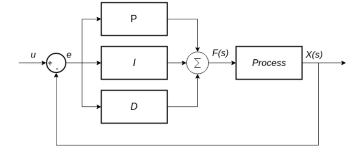
The most common control approach on position control is the classic Proportional-Integral-Derivative controller (PID), which is a feedback controller. The response of this controller is given by:

F(s) = Kp+K_s1+KDsE(s) (2.4)

This controller operates on the application of a proportional term (P), an integral term (I) and a derivative term, D. The proportional gain contributes to the output based on the existing error, while the integral term increases the action output in relation not only to the current error but also the time for which it has persisted. The integral portion guarantees that if the applied force is not sufficient to bring the error to zero, eventually as time passes it will converge to zero.

The derivative term aims at controlling the rate of change of error in the system, reducing the overshoot[28,29,30,31].

The image presented in 2.5 illustrates the context of the application of this controller in a generic system.

Figure 2.5: Context of application of a PID controller in a generic system .

In [20] a simple PID controller is presented to control the altitude of the vehicle while it moves horizontally. It was able to converge the altitude value from a 0.5m to a reference of 0.3m in approximately 3s.

Several other cases of success have been reported relative to the control of AUVs based on the PID approach, demonstrating its effectiveness in this ambit [31,7,18].

In order to control the movement of a profiler, in [1] a speed controller that controls the ve-locities in the z axis and a position controller that allows the control of the vehicles’ position in the z axis were used. A test where the profiler dived to a defined depth completely vertical was performed. An example of an operation performed was the instruction to dive to 0.4m with a speed of 0.1m/s and the vehicle took around 3s to reach the reference, maintaining this value.

These approaches of control reveals rather underwhelming in more complex tasks where the mathematical model is difficult to obtain precisely. Furthermore, the underwater vehicle’s dy-namics can be highly non-linear in a marine environment, making these approaches unable to process efficiently, leading to poor performance of the controller [23]. In some cases, the process of linearization of an underwater vehicle is not enough for the pretended performance.

In order to overcome the problems described many other solutions have been proposed, based on adaptive and/or Fuzzy control.

An improved adaptive hybrid fuzzy control for the horizontal motion was used in [32]. Since it is based on fuzzy logic theory, it does not need a precise mathematical model of the vehicle, being based on fuzzy sets and rules articulated through human expertise and experience. It is called adaptive because it allows the tuning of the parameters online based on the performance of the error’s change. The main improvements are the addition of an integration factor to the

conventional fuzzy controller in order to eliminate steady-state error, and the output of values with nonlinear rules near the region of zero in order to enhance the sensitivity and precision. This approach presented improvements on the response speed, reduced the oscillation magnitude of static phase, higher resistance and robustness against external disturbance compared to a PID controller, resulting in a higher stability of the control system.

In [33] an adaptive sliding mode with PID tuning method is presented. It uses sliding mode control in order to deal with uncertainty, variation and possible disturbances on the parameters of the process, improving the robustness of the control system. The results demonstrated that the designed controller satisfied the need to deal with the non-linearity and uncertainty when controlling the pitch angle of an AUV.

Another possible approach is the adaptive neural networks control. In [23] and [34] propose adaptive neural sliding methods based on the Radial Basis Function (RBF) neural networks. Sim-ulations and tests realized on those articles demonstrate that an adaptive online learning approach based on RBF neural networks allows the identification of the parameters of AUV’s dynamics and induces a better performance compared with the normal adaptive sliding mode.

2.3

Filtering

Besides the control algorithm, the application of filters is a valuable way of removing noise and preparing the information to be given to the control phase, increasing the reliability of the system. Estimations filter are commonly used to enhance the accuracy in the measurement and to filter out high deviations [35, 13]. The Kalman filter is a general error tracking and estimation based filter. At each time interval, the Kalman filter updates its prediction based on the characteristics of the process, then using the measurements obtained through its sensors, the final value is obtained by adjusting the prediction value with the measurement. The more accurate the measurement the more impact it will have in the correction phase. Furthermore, when the vision system could not acquire the information needed to know the state of the system, it can use the prediction given by the prediction phase or even integrates more information coming through other sensors [36].

In [31], in order to deal with the non-linearity of the model of the underwater vehicle the Extended Kalman Filter was used. In this nonlinear version of the Kalman filter, the model can be fined as differential functions and still retrieve the functionality of estimation of the typical Kalman filter.

As stated in [37] in cases of nonlinear systems, non-Gaussian noise distribution, and extreme irregular measurements, the use of other approaches of filtering other than the Kalman filter, like the particle filter, is recommended. The particle filter is the approximated Bayesian filtering al-gorithm based on the Monte Carlo method. The idea of this filter is as follows: It is supposed that the state distribution is known and it is also known its probability density function. Extract N samples in the state space which are called particle and represent the hypotheses. These parti-cles are evaluated using the information gathered by sensors in order to know how likely is that state. After updating each particle, the less likely states are substituted by new samples based on

the most likely existing particles. Over time, the number of particles near the correct state will increase gradually, improving the estimation. In [38], the particle filter is used in order to track an underwater vehicle in a swimming pool. The results concluded that the algorithm achieves real-time and stable moving, and overcomes the shortcomings of a typical Kalman filter.

System overview and implementation

In this chapter, it will initially be presented an overview of the system developed. It will be listed the requirements that were set for this system. Soon after it will be explained how the system was separated into modules and how they were inserted in the overall vehicle’s control system. Posterior to that, the principles, thought process and software architecture used in the implementation of these modules will be presented.

It will be also presented and explained all the work done to implement the features necessary in order to achieve the goal of this system. Furthermore, the methods used to characterize and test the implementation will be described, its results and a critical overview of these results will be presented.

3.1

System design

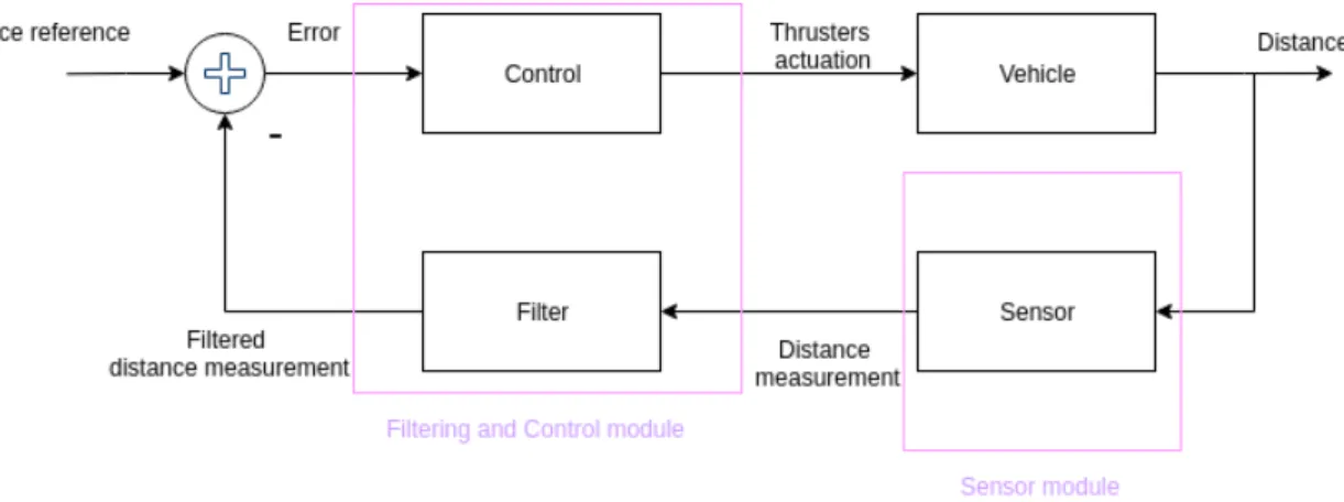
To achieve a system capable of controlling the altitude of an underwater vehicle using sensing based on computer vision, it was developed a module capable of measuring the distance (Sensor module) and a module able to filter the data gathered by the sensor module and capable of using these data to control the distance of the vehicle to an obstacle (Filtering and Control module). Figure3.1 illustrates a block diagram that demonstrates an high level view of the context where these modules are inserted and how they interact with each other.

The diagram shows that the Filtering and Control module and Sensor module are inserted in a distance control loop sequence of a vehicle based on the input of a reference that is compared to the value obtained by the Sensor module after filtering. Based on this comparation difference the control module operates in order to converge the distance of the vehicle towards the reference altitude by deciding the actuation that is necessary to give to the thrusters of the vehicle.

The division on two modules allows the implementation of the two main inherent features of the system (sensing and control) independently and therefore enables the introduction or the improvement of features on any module without imposing significant changes on the other module. This is especially important since it is intended that the sensor module is developed in a way

Figure 3.1: Block diagram of the overall system integrating the modules developed in this disser-tation

that allows its use in other underwater applications other than the control of the distance of an underwater vehicle.

Unlike the Sensor module, the Filtering and Control module was designed and developed based on the vehicle’s properties and the characteristics of the data provided by the Sensor module since its main purpose is the adaptation of the information provided by the Sensor module and its use in order to control the vehicle.

In this dissertation, the underwater vehicle used to test the modules developed was a vertical profiler developed in [1]. The vehicle has approximately 1.35 m of length and a mass of 11.3 kg and its main purposes are the navigation in the vertical axis in order to acquire information related to the water properties and the inspection of the sea floor. An image of the vehicle mentioned is presented in the figure3.2

Figure 3.2: Image of the profiler

Based on the area of application and other limitations related to the vehicle and available material, a set of requirements were imposed to the overall system that was distributed by the two modules. These are presented in the following sections. It is also presented the implementation of those modules and the respective tests performed.

3.2

Sensor module

The Sensor module’s main purpose is the measurement of the distance of the vehicle towards the obstacle based on computer vision. In order to achieve this functionality and guarantee the possibility of utilization of the sensor module in other underwater applications, the module should be able to accomplish the following main requirements:

• _{Since the profiler’s available space is extremely restricted, especially in its extremity where} the Sensor module hardware would be placed, some limitations are imposed on its compo-nents. Specifically, the hardware needed to implement the Sensor module must have less than 12cm of diameter;

• Must use the already chosen camera for the profiler. In3.2.2.1more details of the already integrated camera will be given. Since this camera uses the Vimba SDK (Software devel-opment kit), the software responsible for its configuration and frame acquisition must take into account the software development kit of this camera;

• Provide information about the quality of the measurements acquired;

• It must be possible to dictate the information provided by the Sensor module and be possible to control the operations that are performed;

• The software related to the Sensor module must work as an independent process while running and retrieve data via User Datagram Protocol (UDP) communication;

• Considering the applications that this sensor could be used for, it must produce (acquisition and processing) new measurements at a rate of at least 5 measurements per second.

3.2.2 Solution implemented

3.2.2.1 Hardware

In order to achieve the Sensor module functionality required, it is first necessary to define the hardware components. The sensor device was implemented based on two laser pointer devices placed parallel to one another beside a CCD camera. The choice of using laser pointer devices over all other variations of lasers presented in chapter2is mainly supported by the inherent lower computer demanding and complexity. Relative to the wavelength of the lasers, the software im-plemented to detect the laser dots allow the utilization of the green coloration. That range of wavelength was chosen since it has the best overall performance in underwater laser application as shown in chapter2.

The camera used was the already integrated camera on the profiler, which is a Mako G-125 camera based on the Vimba SDK from Allied Vision [39]. It is well compacted, allows the power-ing over Ethernet, and in full resolution is able to provide 30.3 frames per second. Although it is

able to provide the mentioned frame rate, an underwater Ethernet cable was used in order to gather the information limiting the maximum frame rate to approximately 9 frames per second.

Relative to the laser pointer devices, it was used two green (532nm) laser modules from Odic-Force Lasers [40]. It was performed an adjustment in order to by-pass the switch pressure button in order to work in continuous operation whenever power is applied.

3.2.2.2 Distance calculation method

The solution implemented to calculate the distance of the vehicle towards the obstacle was based on the laser triangulation principle. This method is illustrated in figure3.3.

Figure 3.3: Triangulation method using a laser beam and a video camera [4] .

In figure3.3, R represents the horizontal resolution in pixels of the camera, f is the horizontal focal length measured in pixels, β the angle between the laser beam and the optical axis, P the pixel where the laser point is projected on the image plane and B the fixed distance between the optical axis and the laser pointer.

The distance to the obstacle (D) can then be given by: tanΘ = R 2 f (3.1) 2P − R 2 f = Dtanβ − B D (3.2) D = BR Rtanβ − (2P − R)tanΘ (3.3)

Analyzing the technology involved, the calculation using only one laser pointer device is enough to retrieve the pretended distance. The choice of using two laser pointer devices in the

sensor device is justified by the introduction of redundancy, increasing the reliability of the system and the quality of the measurements by merging the 2 values.

3.2.3 Software architecture

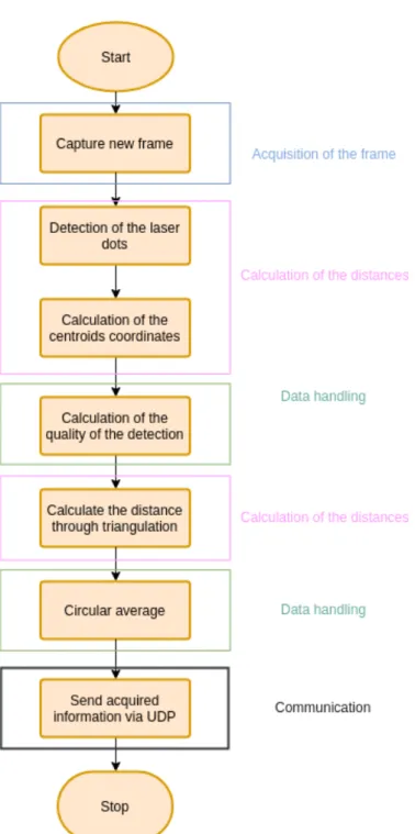
In order to accomplish the requirements presented for the Sensor module, the software developed was structured to perform 4 main features: Acquisition of the frame; Calculation of the distances; Data handling; Communication.

The first feature is responsible for the configuration and communication with the camera de-vice and the acquisition of new frames. Each time a new frame is ready to be used, it is sent to be processed.

The Calculation of the distances feature purpose is the process of the image captured in order to acquire the distance towards the object. It is divided into 3 phases: detection of the laser dots on the image; calculation of the centroids of the laser dots; triangulation method in order to compute the distance. First, the image is processed using image processing methods in order to obtain a left and right segmented image containing only the left and right detected laser respectively. Then, the centroid of each laser dot is obtained and sent to the last phase where based on laser triangulation, a distance towards the obstacle is obtained for each dot in use.

The Data handling is responsible for two main operations: calculation of the quality of the de-tection of the laser dots and application of certain operations based on the software configuration, for example, application of a circular average on the measurements.

All the information acquired is then sent to the user through UDP communication in the last phase and the software awaits a new frame to process (Communication).

Figure3.4illustrates the procedures that occur in a generic execution of the software from the acquisition of the frame to the dispatch of the data to the user.

Figure 3.4: Example of a generic high-level execution of the software related to the Sensor module .

3.2.4 Acquisition of the frame

For the implementation of this feature the software presented in [41] was used. It allows the configuration of the parameters of the camera, for example, frames per second, resolution, and exposure time. It also allows the acquisition of the images of any camera that uses the Vimba SDK. Its use in this dissertation was authorized by its authors, but since the software was not developed during this dissertation, its design and implementation is not going to be detailed.

3.2.5 Calculation of distances

The software responsible for the distance calculation is divided into 3 phases: Laser dots detection, centroid calculation, and triangulation calculation. All these 3 phases were implemented in a class called ImageProcessing. Furthermore, this class posses other methods that improve the quality of the operation and increase the amount of control and information that is extracted.

The main methods included in this class are:

• slot confImageProcessing - slot that is called when a signal symbolizing that a UDP frame referent to the configuration of the image processing process was received. This UDP frame is used to enable or disable the service responsible for the distance calculation by the user during the operation;

• loadImageProcessingConfig - method that reads a XML (Extensible Markup Language) file that can be edited in order to configure all the operations and information that are relevant to be acquired;

• slot ProcessImage - slot that is called when a signal symbolizing that a new frame is ready is sent from the acquisition phase;

• calcDistance - method called by the slot ProcessImage that receives the new image in order to initiate the sequence of processing. It is responsible for the calculation of the distances and then for calling the method capable of transmitting the information acquired to the user; • detectDots - method responsible for the creation of two segmented images that only contains

the left and right laser dots detected separately;

• _{calcCentroidsDots - method that calculates the centroid coordinates of each of the laser dots} detected;

• Triangulation - method that applies the triangulation operation in order to compute the dis-tances;

• calcQualityFactor - method responsible for calculating the quality factor of each measure-ment;

• calcCircularAverage - method that calculates the circular average of the last N measure-ments. The value of N is specified through the configuration file.

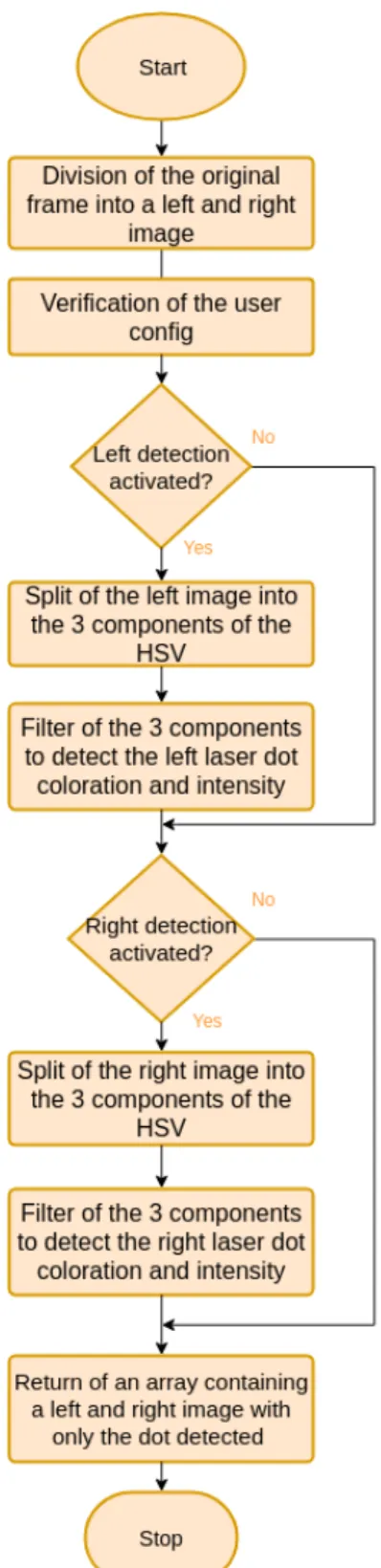
3.2.5.1 Laser dots detection

The method detectDots is responsible for the laser dots detection. The order of operations is as described in figure3.5:

Figure 3.5: Flowchart of the operations that occur in the detectDots method .

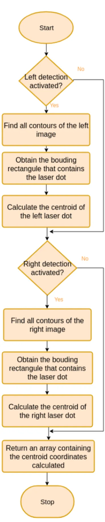
3.2.5.2 Centroid calculation

The method calcCentroidsDots is responsible for the calculation of the centroid coordinates. The order of operation is present in figure3.6:

Figure 3.6: Flowchart of the operations that occur in the calcCentroidsDots method .

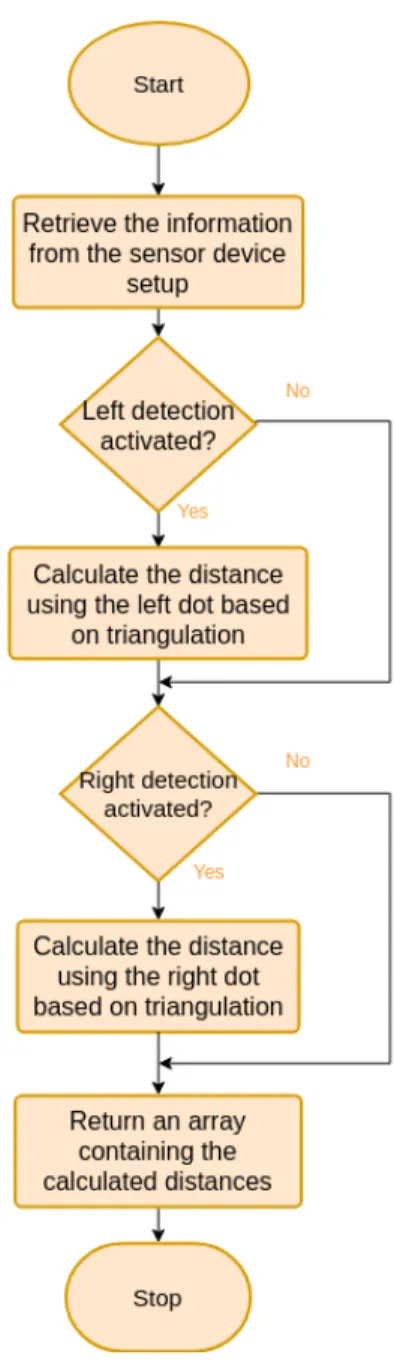
3.2.5.3 Triangulation calculation

The computation of the distances is executed by the Triangulation method. Figure3.7shows the sequence of actions that take place in this calculation.

Figure 3.7: Flowchart of the operations that occur in the Triangulation method .

3.2.6 Data handling

After the computation of the centroid coordinates of the laser dots, the method calcDistance calls the method calcQualityFactor that retrieves a quality factor of each laser dot detected based on its location and circularity. If the quality factor is considered lower than a determined threshold, the detection of that specific laser dot is treated as not successful and the distance related to that laser

dot is not calculated. After the calculation of the distances by the Triangulation method, the results of the detection and the distances calculation are examined in order to decide what information to send to the user. Each operation has the capacity of detection errors and inserting error codes in the procedure that can be detected by this phase. The information sent is dependent on how successfully the calculation was.

3.2.7 Communication

After the determination of the information that is going to be sent to the user, an array is filled with all the information demanded in the software’s configuration. The format of this array is as follows:

Table 3.1: Communication array format

Vector position Information

0 Left dot distance

1 Right dot distance

2 Average or circular average

3 Quality factor of the left dot detection 4 Quality factor of the right dot detection

The information of this array depends on the configuration of the software, quality of the measures and on how successfully the overall procedure was. For example, if the left or right detection is disable on the configuration, in the positions 0 or 1, correspondingly, the user will receive the value -2, indicating that the functionality was not enabled in the configuration file. The same is verified for the rest of the array positions since the average, circular average and quality factors calculations can be enabled or disabled in the configuration file.

In case of any type of error detected during the calculation of any of the information of those positions, the user will receive the value -1, indicating that the data acquired for that array position was considered not reliable nor valuable. This can occur in a situation of internal errors, fail on the detection of the laser dots or centroid coordinates or if the quality factor is considered below a certain value.

After filling the array mentioned, this array is sent via UDP communication. This functionality was implemented by modifying and adding necessary methods to a class present in the software used in [41] already mentioned, class named Protocol. This class originally allowed the features of sending and receiving UDP packages. Minor changes were made to some methods already present in this class and the following 3 methods were added:

• A method that allows the user to initiate and terminate the calculation of the distance through UDP communication (named send_ConfigImageProcessing);

• A method used by the calcDistance method in order to fill a package that contains the array of information following certain rules to make it clear for the user the order of the informa-tion transmitted (called send_DistCalc);

• A method that allows the user to receive the information calculated by the Sensor module through UDP (ReceiveDistance).

The class Protocol mentioned and a XML file are the interface elements that allow a user to communicate and control the Sensor module. It is needed of the method socket present in the Protocol class in order to create a socket capable of communicating with the Sensor module and the use of the method send_ConfigImageProcessing containing the command to enable or disable the calculation of the distance. A C++ example of this procedure is illustrated in figure3.8.

Figure 3.8: Example of the interaction with the Sensor module in order to enable its operation .

Furthermore, an XML file present in the Sensor module package must be filled as shown in figure3.9.

Figure 3.9: Configuration XML file example .

These steps will initiate the Sensor module operation. In order to receive the information, the user uses the ReceiveDistance method present in the Protocol class as presented in the C++ example in figure3.10.

Figure 3.10: Example of the use of the ReceiveDistance method .

3.2.8 Characterization and tests

In order to characterize and test the sensor module, it is first necessary to know the limitation of the technology used in the distance calculation. Through the triangulation method it is known that the accuracy of the measurements is inversely proportional to the distance of the obstacle. This can be demonstrated by the analysis of the distance procedure shown in3.2.2.2:

D = BR

Rtanβ − (2P − R)tanΘ (3.4)

Considering the angle between the laser beam and the optical axis (β ) equal to 0, the equation presented in3.5is given by:

D = _RB f

2−P

(3.5) The denominator on the equation presented represents the distance in pixels between the pixel where the laser point is projected on the image plane and the center point of the image (∆ dpixels).

Since the value of B and f are constant values related to the setup of the sensor device, the only determinant factor is the value of ∆ dpixels. Since this value depends only on which pixel the

laser dot is detected, it is then possible to assert that the range of values of the distance obtained is "discrete" and has an error equal to the distance necessary to go through that makes the detection of the laser to be in the forthcoming pixel. In table3.2 it is illustrated the value of the inherent error caused by the use of this method for 4 different distances for B equal to 4cm and f equal to 1615. The values for B and f have no practical meaning and are therefore only valuable in order to exemplify the topic described.

Using the results from table3.2is possible to verify that the error is increasing with the increase on the distance as expected.

It is also necessary to know the error induced through the utilization of non-ideal components and possible software limitations. In order to quantify these errors, a methodology of testing is

Table 3.2: Inherent error caused by laser triangulation

∆dpixels D for ∆ dpixels ∆dpixels + 1 D for ∆ dpixels + 1 error error(%)

250 0.258m 249 0.259m 0.1cm 0.39

60 1.077m 59 1.095m 1.8cm 1.69

36 1.794m 35 1.846m 5.2cm 2.90

21 3.076m 20 3.230m 15.4cm 5.00

used to ensure that it is possible to not only calibrate the sensor module but also examine the possible error present on the measures.

The structure set up in order to test the Sensor module is illustrated in the images3.11and

3.12.

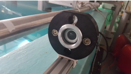
Figure 3.11: Structure containing the camera and the laser devices .

The structure illustrated contains the camera, laser pointer devices mentioned in3.2.2.1fixed into a 3 m structure marked each 10 cm and a movable target.

The first phase of tests is the determination of the divergence of the camera relative to the target. In order to do so, the target contains a center mark that can be compared to the center of the image that is being captured by the camera. A series of tests were performed from the range of 10 to 250 cm, moving the target 20cm between each test. The results obtained are presented in table3.3.

Figure 3.12: The full structure underwater, containing the target on the left .

Table 3.3: Deviation of the camera angle of view D Deviation of the center

0.10 m 0.3 cm 0.30 m 0.7 cm 0.50 m 1.1 cm 0.70 m 1.6 cm 0.90 m 2.1 cm 1.10 m 2.6 cm 1.30 m 3 cm 1.50 m 3.4 cm 1.70 m 3.7 cm 1.9 m 4.1 cm 2.1 m 4.4 cm 2.3 m 4.8 cm 2.5 m 5.1 cm

By analyzing the information from table3.3it is possible to calculate a linear regression that translates the increment of the deviation with the increase of the distance towards the obstacle. The equation calculated capable of defining the deviation in meters is presented in3.6.

Deviation = 0.02033 × D + 0.001956 (3.6)

devices were placed with 4cm to the center each and it is expected that as the distance increases this distance on the target will change due to the angle of the laser devices. The measurement of this divergence took into account the deviation of the camera. For each test, the distance of the laser beams on the target towards the center (Dleft-centerand Dright-center) was calculated and the

results are presented in table3.4.

Table 3.4: Deviation of the lasers D Dleft-center Dright-center 0.10 m 4.2 cm 3.8 cm 0.30 m 4.4 cm 3.5 cm 0.50 m 4.7 cm 3.2 cm 0.70 m 5.0 cm 2.9 cm 0.90 m 5.3 cm 2.6 cm 1.10 m 5.5 cm 2.4 cm 1.30 m 5.7 cm 2.2 cm 1.50 m 6.0 cm 1.9 cm 1.70 m 6.3 cm 1.7 cm 1.9 m 6.7 cm 1.4 cm 2.1 m 7.0 cm 1.1 cm 2.3 m 7.3 cm 0.8 cm 2.5 m 7.5 cm 0.6 cm

As expected the rate of change of the distance of the lasers towards the center is constant due to the angle of the lasers being constant. Therefore, it is possible to calculate a linear regression of this divergence and use it in order to correct it. The linear regressions obtained were the following: Dleft-center=0.01404 × D + 0.03990 (3.7)

Dright-center= −0.01316 × D + 0.03872 (3.8)

After these two procedures of calibration, a series of tests were performed from the range of 10 to 250 cm, moving the target 20cm between each test in order to validate the performance of the Sensor module. The deviation study performed previously was used in order to correct the distance of the lasers towards the center at each calculation of the distance. This means that initially, the software uses the value of 4 cm for the distance of the lasers, but after each distance calculation, the value obtained is inserted in the linear regression equations in order to retrieve the value of the actual deviation of the laser dots towards the center.

The results obtained for the distance calculated using the left laser dot (Dl) and right laser dot

(Dr) are presented in the table3.5.

Table 3.5: Results obtained for sensor performance

D Dl Dr Errorl Errorr 0.10 m 0.1004 m 0.1014 m 0.4 mm 1.4 mm 0.30 m 0.3011 m 0.3017 m 1.1 mm 1.7 mm 0.50 m 0.4942 m 0.5027 m 5.8 mm 2.7 mm 0.70 m 0.7022 m 0.6889 m 2.2 mm 1.1 cm 0.90 m 0.9106 m 0.8769 m 1.06 cm 2.31 cm 1.10 m 1.0832 m 1.0737 m 1.68 cm 2.63 cm 1.30 m 1.2795 m 1.2785 m 2.05 cm 2.15 cm 1.50 m 1.4908 m 1.4712 m 0.92 cm 2.88 cm 1.70 m 1.6958 m 1.7196 m 0.42 cm 1.96 cm 1.9 m 1.8983 m 1.8742 m 0.17 cm 2.58 cm 2.1 m 2.1740 m 2.1606 m 7.4 cm 6.06 cm 2.3 m 2.3579 m 2.2253 m 5.79 cm 7.47 cm 2.5 m 2.5635 m 2.4225 m 6.35 cm 7.75 cm

The results show that the sensor is working as intended showing an error within the range mentioned in table 3.2, where the deviations compared to that range is essentially due to the infrastructure, where the camera, obstacle and even the lasers might have suffered small changes in their position during the tests. Furthermore, some error in the measurement of the lasers and camera deviations that were acquired manually have a significant impact on the measurements obtained.

Figure 3.13: Measurements obtained by the left laser dot .

Figure 3.14: Measurements obtained by the right laser dot .