Investigating climbing fiber activity during locomotor learning

UNIVERSIDADE DE LISBOA

FACULDADE DE CIÊNCIAS

DEPARTAMENTO DE FÍSICA

Investigating climbing fiber activity during locomotor learning

Hugo Viana Bettencourt

Mestrado Integrado em Engenharia Biomédica e Biofísica

Perfil em Sinais e Imagens Biomédicas

Dissertação orientada por:

Prof. Dr. Alexandre Andrade

Abstract

Patients with cerebellar damage invariably display impairments in locomotion. The cerebellum is vital for calibrating motor patterns, and it achieves this by integrating neural signals from two main inputs: mossy and climbing fibers. Whilst the former incorporates contextual sensory information, the latter informs the cerebellum about movement errors. These error signals, that originate in the contralateral inferior olive, are essential to promote changes in motor patterns that eventually lead to motor learning. However, it is still not clear how exactly these climbing fibers are involved in complex tasks that require the coordination of different body parts. In this work, we aim to understand the role of the climbing fiber signals in a locomotor learning task. Here, we developed methods to 1) optogenetically perturb climbing fiber activity, and 2) image climbing fiber responses in the cerebellar cortex using calcium imaging. Preliminary results from the optogenetic experiments highlight the necessity of successfully targeting climbing fibers with a combined genetic and anatomical approach to achieve sufficient specificity. In the imaging experiments we demonstrate successful single-cell identification and signal extraction in the cerebellar cortex. This work provides tools to study the role of the climbing fibers during locomotor learning.

Resumo

Em tarefas quotidianas, os membros do nosso corpo encontram-se perfeitamente coordenados de

modo a atingir movimentos suaves e eficientes sofre

em suscitado

o interesse n

planeamento de movimentos, e outras tarefas mais complexas. cerebelar

celular relativamente simples e estereotipada, que se repete ao longo da sua estrutura. Dois inputs esta : as fibras musgosas e as fibras trepadeiras. Enquanto as primeiras transmitem contextual acerca do a

sinais de erro provenientes de uma estrutura cerebelar no tronco cerebral contralateral, inferior. A atividade dos dois tipos de

um tem n fibras musgosas

Purkinje o cerebelar fibras paralelas. Estas

comunicam com as c lulas de Purkinje, o breves, chamados picos simples, acima dos 60Hz). Em contraste, cada fibra trepadeira entra

apenas , levando a que esta produza um sinal

- excit rio elevado, caracterizado por s pico

complexo picos simples (cerca

de 1Hz), levando a uma pausa dos picos simples empo.

As fibras trepadeiras enviam sinais de erro do para o cerebelo e pensa-se que estes sinais a cabo a aprendizagem motora. Isto foi verificado em tarefas

motoras simples, como a estabiliz . No entanto, sabemos como

envolvem de todo o

corpo.

Neste estudo um paradigma experimental que avalia

locomotora utilizando murganhos como modelo animal. Nesta tarefa, denominado passadeira de cinta dupla, o murganho anda num corredor estreito por cima de duas cintas transparentes (uma de cada lado do corpo) cujas velocidades podem ser controladas independentemente. Com um espelho angulado a gravar simultaneamente a parte debaixo e de lado do corpo do murganho enquanto este anda no corredor. Quando uma das cintas do que a outra

conhecida como split

. Com , o murganho aprende um novo

locomotor que reduz a assimetria imposta. Subsequentemente, quando voltamos

em ambas as cintas denominada por tied observamos novamente uma assimetria, mas no aftereffect

locom split, e que este foi

de algum modo memorizado.

Para conseguirmos estudar o impacto das fibras trepadeiras na aprendizagem locomotora, , de modo a tentarmos perturbar a atividade destes ne

inferior utilizando uma linha de murganhos denominada Thy1-ChR2-YFP. Nesta linha, as mbranar denominada channelrhodopsin-2 que muda

na

era que os animais andassem no setup experimental enquanto ativ duas s de laser diferentes: 2Hz e 10Hz.

uma significativa da aprendizagem locomotora evidente pela do aftereffect.

p c a

a aprendizagem locomotora.

, quando a era ipsilateral.

Esta lateralidade dos resultado de que

os sinais de erro origem contralateral.

o

olivar inferior

-o especifici

mai

-ChR2-YFP e AAVretro-Jaws. A primeira envolvia a

de channelrhodopin-2 restringida a o . Nesta

dos dois murganhos de um outro projeto . Verificou-se uma di tados de ambos, tendo a histologia evidenciado um

-nos a concluir que, para identificarmos se a ma

deve ser feito com

posicionamento correcto das fibras. , envolvia administradas no

elar para expressar o

uma fonte de luz amarela. Os nossos resultados

obter histologia destes animais, temos ainda a fibras

trepadeiras, nem do posic .

Para tod recorr atividade das fibras

trepadeiras. No entanto, ,

os nossos resultados, embora promissores, s.

Para avaliar a atividade das fibras trepadeiras durante a aprendizagem na passadeira de cinta dupla, sinais de induzidos por picos complexos. Esta plataforma

U colcoado no meio da roda, permite-nos filmar

simultaneamente a parte de baixo e a parte lateral .

nova plataforma demonstrou a capacidade para filmar o comportamento do animal eo com

sinais Purkinje.

e com sucesso a

estimativas da sua atividade neuronal.

Neste projecto procurou- fibras trepadeiras na

base para futuras ex com o objectivo de identificar, pertubar e visualizar a sua atividade durante aprendizagem locomotora.

Palavras-chave: cerebelo, fibras trepadeiras, locomo , aprendizagem motora, optogenetica, microscopia de

Acknowlegdements

I would like to start by thanking Dr. Megan Carey for the opportunity to be apart of her lab for almost 2.5 years and letting me conduct incredible investigative work, with a lot of patience and enthusiasm along the way.

To my internal supervisor Dr. Alexandre Andrade I thank you for the support you gave me this past few years, especially throughout my thesis project. Your knowledge, patience and help throughout my college years has shaped me to the person I am today.

For all the members of the Carey Lab: Ana G., Ana M., Catarina, Dana, Diogo, Dennis, Dominique, Hugo, Jovin, Marta, Tatiana and Tracy; a huge thank you for the debates, coffee sessions, picnics and lab meetings that made feel at home and guided me to create the story I present in this thesis. Without your help and tutorship, I would have not been able to perform at my best capacity. However, I dedicate this work to Hugo Marques. With your supervision, motivation and enthusiasm I had the change to learn more than I imagined and present a work that I m extremely proud of. I will take your advice and knowledge with me for the rest of my life.

A special thank you to the amazing friends I made at the Champalimaud Foundation: Daniela, Diogo, Margarida and Marta. Your support and our daily lunch shenanigans motivated and helped me carry on despite situations where I thought I couldn t anymore.

To Beatriz and Teresa, my friends for life: you were responsible for keeping me sane and happy this past year. Just an hour a week was enough for me to unwind and forget all the problems that were inherent to the scientific process. I hope you ll be there always, because god knows I need it.

Without my family and their support none of this would have been possible. For my mom I thank you for the huge support, even when you didn t know or understand what I was doing. You have shaped my career and life in an incredible way and I couldn t thank you enough. To my grandma, I send such a huge gratitude for listening when I just wanted to talk and in helping in any way, shape or form. To my sister Sara, that is the biggest example of persistence and courage to take the world by the horns and controlling it, I send my sincere gratitude. To all, I love you.

And finally to Afonso, my rock and source of emotional support. Your presence, even thousand of miles away for this past year, was vital for the success of this thesis. Thank you for everything and I love you.

Contents

1.

Introduction

1.1. The cerebellar cortex: cell types, neural connectivity, and electrical activity ... 1

1.2. Functions of the cerebellum: motor coordination and learning ... 3

1.3. Cerebellar gait ataxia: how is the cerebellum involved? ... 5

1.4. Interlimb coordination and learning ... 5

1.5. Project objectives ... 6

2.

Methods

2.1.5. Split-belt treadmill protocols ... 11

2.1.6. Laser stimulation protocols ... 13

2.1.7. Data analysis ... 13 2.1.8. Histology ... 13 2.2. Imaging ... 14 2.2.1. Surgical procedures ... 14 2.2.2. Experimental setup ... 14 2.2.3. Experimental protocols ... 15

2.2.4. Rotary treadmill tracking algorithm ... 15

2.2.5. Imaging analysis ... 15

3.

Results

3.1.1. Thy1-ChR2 ... 19

3.2. Behavioral and Imaging setup... 31 3.2.1. Behavioral platform ... 31 3.2.2. Imaging analysis ... 33

4.

Discussion

4.2. Behavioral setup and imaging analysis ... 37

4.2.1. Behavioral setup ... 37

4.2.2. Imaging analysis ... 37

5.

Conclusion ... 39

List of Figures

Figure 1.1 Graphical representation of the cerebellar circuit ... 2

Figure 1.2 Electrical activity of the cerebellar Purkinje cells recorded intracellularly ... 2

Figure 1.3 Learning curves gathered from a task that consisted in hitting a fixed target with a dart ... 4

Figure 2.1 Split-belt treadmill for mice ... 9

Figure 2.2 Illustration of a stride cycle in a mouse ... 9

Figure 2.3 Example of tracks gathered by the LocoMouse tracking algorithm ... 10

Figure 2.4 Short protocol performed in the Split-belt treadmill for the Thy1-ChR2-YFP and VGlut2-ChR2-YFP manipulations ... 12

Figure 2.5 Long protocol performed in the Split-belt treadmill for the AAVretro-Jaws manipulation ... 12

Figure 2.6 Rotary treadmill experimental setup. ... 15

Figure 2.7 Mukamel cell sorting algorithm divided into five stages ... 16

Figure 2.8 Example of the selection process applied to the gathered PCs ... 17

Figure 3.1 Control vs 2H RF stimulation in Thy1-ChR2-YFP transgenic mice ... 20

Figure 3.2 Control vs 10HzRF stimulation in Thy1-ChR2-YFP transgenic mice ... 22

Figure 3.3 Control vs 10HzLF stimulation in Thy1-ChR2-YFP transgenic mice ... 23

Figure 3.4 Baseline analysis between the control and stimulation protocols in the Thy1-ChR2-YFP transgenic mice ... 25

Figure 3.5 Control vs 10HzRF stimulation in VGlut2-ChR2-YFP transgenic mice ... 27

Figure 3.6 Histology results gathered from the two VGlut2-ChR2-YFP transgenic animals ... 28

Figure 3.7 Baseline analysis between the control and the 10Hz RF protocols in the VGlut2-ChR2-YFP transgenic mice ... 28

Figure 3.8 Control vs 0.5Hz laser frequency stimulation in wild type mice expressing AAVretro-Jaws ... 30

Figure 3.9 Tracking results from a mouse walking on top of the rotary treadmill ... 32

Figure 3.10 Example of the Mukamel algorithm pipeline... 33

1.

Despite the constant changes in their body and environment, animals maintain a stable and efficient locomotor pattern effortlessly. This is a complex task, since it needs every body part to be perfectly coordinated across space and time. The cerebellum is believed to be crucial for such a coordinated movement, since cerebellar patients are known to display gait ataxia [1] [3]. However, it is still unknown how the cerebellum achieves this.

The work presented in this thesis aims to manipulate the activity of the climbing fibers to perturb sensory error signals that are thought to be involved in locomotor learning. We also implemented a new experimental setup that will allow us to image the activity of these cells during a locomotor learning task.

This chapter is organized into four sections. The first section presents a detailed description of the cellular architecture of the cerebellar cortex. The second section analyzes the functionality of the cerebellum and its cellular components. The third section gives an overview of how the cerebellum is involved in motor coordination. The fourth section describes how locomotor learning can be studied in a laboratory environment.

1.1. The cerebellar cortex: cell types, neural connectivity, and electrical activity

The cerebellar cortex has a relatively simple and stereotyped cellular structure, which facilitates Neuroscience researchers to locate specific cell types and analyze their activity during behavioral tasks [4]. To achieve this goal, techniques such as genetical manipulations, electrophysiology, and neuroimaging have been applied in an attempt to understand how the neural connections between the existing neurons delineate the function of this brain region [3].

Figure 1.1 shows a schematic of the cerebellar circuit. Two excitatory pathways convey information to the cerebellar cortex. The mossy fibers carry contextual information originating in several brain regions. In contrast, climbing fibers carry error signals that originate in the contralateral inferior olive, a brain structure located at the level of the brain stem [3], [5], [6]. Both input systems make distinct synaptic connections with the Purkinje cells the sole output of the cerebellar cortex. The mossy fiber pathway indirectly connects with the output neurons via granule cells. Each granule cell then projects to Purkinje cells in a T-shape branch. These projections are named parallel fibers. They distribute the information from individual mossy fibers to many Purkinje cells [3]. However, this is not the case for the climbing fibers. Each climbing fiber synapses directly with 1 to 10 Purkinje cells, with each output neuron only receiving projections from a single climbing fiber [4]. This establishes a highly specific connectivity between the climbing fibers and the cerebellar Purkinje cells [3].

Figure 1.1 Graphical representation of the cerebellar circuit. The neurons in orange and pink carry information to the cerebellar cortex (mossy and climbing fibers, respectively). Green cells represent the granule cells and their corresponding parallel fibers, which then forms synaptic connections with the Purkinje cells (represented in purple). The Purkinje cells enter in contact with the deep cerebellar nuclei (DCN - blue), which then connects with other brain areas, such as the motor cortex. Adapted from [7].

From a physiological point of view, each input system impacts the Purkinje cell activity in distinct ways. The mossy fibers produce brief single action potentials, also named simple spikes, at a relatively high frequency (spontaneous activity ~60Hz) [3]. These signals are thought to produce an impact on motor commands [7] [9]. On the other hand, the climbing fiber synapse, considered one of the most powerful connections in the vertebrate nervous system, has a higher excitatory influence in the Purkinje cell activity, and it is believed to be responsible for inducing motor learning [5]. The impulses carried by the climbing fibers yield an extremely powerful excitatory postsynaptic potential in the Purkinje cells [6]. These discharges, named complex spikes, occur at a relatively low frequency (spontaneous activity ~1Hz) and are characterized by a large initial amplitude, followed by a sequence of partial spike responses, named spikelets, and a prolonged period of depolarization, called an inactivation response [10]. During this inactivation response, the mossy fiber activity gets silenced [11]. The difference between the two types of activity can be observed in Figure 1.2.

Figure 1.2 Electrical activity of the cerebellar Purkinje cells recorded intracellularly. (1) A brief single action potential, named simple spike, is produced by the mossy fiber inputs via the parallel fiber projections; (2) A discharge characterized by a large initial amplitude, with a posterior sequence of partial spike responses, named spikelets, and a prolonged period of

1.2. Functions of the cerebellum: motor coordination and learning

The inability of reaching a fixed target, a delay in the initiation of movement and a lack of coordination between limbs are common and well-documented symptoms in patients with cerebellar damage [1] [3]. Based on these abnormalities, several studies have attempted to understand exactly what is the function of the cerebellum.

Makoto Fujita has proposed the cerebellum to act as an adaptive filter where each of the mossy fiber inputs is characterized by a specific weight. These weights are adjusted once in the presence of a signal carried by the climbing fibers. This signal is defined by the difference between the motor command being performed and the desired motor goal [12]. Once this difference reaches zero, the climbing fiber activity loses its impact and the motor learning process is terminated.

As quick coordinated movements cannot be performed under pure feedback control, due to the slow feedback process and small gains, theories extended beyond this simple feedback loop [13]. In these studies, the cerebellum is defined as a predictive machine [14], [15]. To update our motor commands and achieve a desired goal, the cerebellum needs two essential components: sensory inputs that send copies of our motor commands and errors that emerge from the performance of these commands. The mossy fibers send the motor copies and the climbing fibers ensure that the motor errors are being relayed into the cerebellar cortex. The incorporation of both components computes a sensory signal that predicts the outcome of movements and compensates for eventual errors [13]. This predictive function of the cerebellum may be observed in eye-blink conditioning studies, where animals learn to associate a neutral stimulus (e.g., a LED light) to a blink evoking stimulus (e.g., an air puff). However, in this case, the mossy fibers do not send a copy of the motor command. Rather, they send the information related to the timing of the neutral stimulus. With time, the incorporation of both mossy and climbing fiber signals will lead to a motor response that suffers a shift in time as the animals learn to predict the air-puff [16] [18].

David Marr proposed the climbing fibers as the responsible components for the motor learning process [4]. The climbing fiber activity would drive synaptic plasticity at the level of the Purkinje cells. This plasticity was termed LTP long term potentiation due to the facilitation of certain parallel fiber synapses that, in the correct pattern, would result in the desired motor output. Later, James Albus demonstrated certain similarities to role of the climbing fibers was different according to him. The synaptic plasticity induced by the climbing fibers would elicit a weakening of the parallel fiber synapses. This process was termed LTD long term depression [19], with a later study showing evidence of this process [20].

Despite differences between both theories, Marr and Albus shared a common idea: the cerebellum functions as a spatial pattern identifier with an ability to change its synaptic configurations when necessary [21]. Albus termed the climbing fibers as a teacher in the context of motor learning, by

to the cerebellar Purkinje cells [19].

at the center of the motor learning process for simple motor behaviors. In VOR (vestibulo-ocular reflex) studies, any alteration in the stabilization of an image in the retina is compensated by a gain change defined as the ratio between eye and head velocities. This motor learning process requires

William Thach delved into a more complex motor task [25]. In his work, humans had to learn to hit a target with a pair of vision impairment goggles that shifted their normal line of sight. In healthy subjects, once the goggles were introduced (first dashed line in Figure 1.3a), Thach observed a motor error (or an initial error) that was reduced with time as the individuals recalibrated their arm movements. Then, after the goggles were removed (second dashed line in Figure 1.3a), another motor error was observed but in the opposite direction (or an aftereffect) indicating that the motor alterations were retained when they had the goggles on. Yet, with time, the execution of the task returned once again to normal. This constitutes the basis of the motor learning process: a continuous improvement of the coordination between different body parts to achieve a goal; with the learning curve illustrated in Figure 1.3a indicating the normal behavior during a motor learning task.

Surprisingly, once patients with a damaged inferior olive (IO) were introduced to the task, the authors gathered a different set of results (Figure 1.3b). The first motor error was shown once the goggles were introduced, but with no improvement as time went by. Also, with the removal of the goggles, the performance returned immediately to normal as if no changes in the arm movement had happened. This experiment suggests that motor learning is impaired in the absence of climbing fiber activity.

Figure 1.3 Learning curves gathered from a task that consisted in hitting a fixed target with a dart. The x-axis refers to the throws performed by the human experimentee. The y-axis mentioned the angular error that was measured from each throw. The first dashed line corresponds to the moment when the vision impairment goggles were introduced, and the second dashed line when the goggles were removed from the experiment. A: Performance of a healthy subject. When the goggles were introduced, a motor error was evident due to the need of a recalibration of the arm movements (initial error). With time this error got smaller. Then, once the goggles were removed, another error in the opposite direction was noted, indicating that the motor alterations were retained (aftereffect). B: Performance of a patient with a damaged inferior olive. We observe an error once the goggles were introduced, but with no improvement with time. Also, no error was recorded once the goggles were removed from the experiment. With no climbing fiber activity the experimentee lost the ability to perform the task. Adapted from [25].

1.3. Cerebellar gait ataxia: how is the cerebellum involved?

As we showed in the previous section, the climbing fiber inputs were shown to be vital for learning to take place in simple motor tasks, with Thach demonstrating that without these cells the ability to perform his eye-hand coordination task was lost. However, gait ataxia, a common thread in cerebellar patients, has yet to be described.

Machado and Darmohray analysed the locomotor coordination in mice with Purkinje cell degeneration (pcd) as they walked along a transparent corridor [2]. Like cerebellar patients these mice showed to be ataxic. After accounting for body size and walking-speed differences between the control and mutant groups, the forward movements of the individual paws were surprisingly similar. However, the authors noted a complete disruption of the normal pattern of whole-body coordination. These results show us that gait ataxia that results from cerebellar damage is characterized by the lack of coordination between body parts, and not by the movements of the individual limbs. The authors argued that this effect in the individual limbs reflected on the existence of compensatory neural mechanisms originated from the complete loss of Purkinje cells.

1.4. Interlimb coordination and learning

With the whole-body coordination impaired in cerebellar gait ataxia, its analysis has become a priority in cerebellum studies. Reisman and Bastian both proposed human tasks aimed to investigate our ability to learn new motor patterns [26], [27]. These tasks involved a split-belt treadmill that allows us to induce perturbations in locomotor symmetry. In this paradigm, each belt underneath the feet of the experimentee is controlled by distinct motors. Once one of the belts goes faster than the other, the locomotion become asymmetrical and a new motor pattern must be implemented.

In these split-belt conditions, the coordination between limbs gets adjusted with time to once again achieve an efficient gait [14], [26]. Both authors demonstrated the learning curve similar to

study (see Section 1.2 Figure 1.3). As the speed ratio between the belts changes, we observe a motor error (initial error) that decreases with time. Once the 1:1 ratio returns there is another motor error, but in the opposite direction (an aftereffect), indicating that the newly acquired motor pattern was implemented and memorized. With time, this motor error also diminishes until we achieve the original stable gait.

Darmohray successfully adapted a version of the split-belt treadmill to mice ([28]), showing results consistent with those observed in the human studies by Reisman and Bastian. Figure 1.4 illustrates an example of a locomotion parameter used to measure the symmetry between the front limbs of the mouse.

The represented learning curve are what

Figure 1.4 Learning curve demonstrating the symmetry between the front paws of the mouse. The grey patch represents the trials where each belt had a different speed (split trials). We observe an initial error once this condition is placed, with an improvement as time goes by. When we return to the normal conditions we observe another motor error in the opposite direction named an aftereffect. Adapted from [28].

1.5. Project objectives

As described, climbing fibers have been hypothesized to send error signals to the cerebellar cortex, thus providing support for motor learning. The goal of this project is to understand the role of the climbing fibers during locomotor learning. To achieve this, we used the mouse model and implemented techniques to either perturb or image the activity of these cells during a locomotor learning task.

To perturb climbing fiber activity we attempted three optogenetical manipulations, while the animals underwent the split-belt learning protocol ([28]). We used optogenetics to either stimulate or inhibit climbing fibers. By stimulating with a frequency ten times higher as the normal baseline, we expected these cells to lose their ability to send their well-timed error signals and thus impairing motor learning. And by inhibiting them, we expected to abolish error signals, a situation alike what Thach observed in his work, and thus also impair motor learning.

To image climbing fiber activity during locomotion, we built a new experimental setup consisting of a freely moving rotary treadmill and a wide-field fluorescence microscope. Our objective was to allow a mouse to walk while head-fixed on top of the treadmill, allowing the imaging of the climbing fibers to take place. We successfully incorporated the paw-tracking algorithm used in the lab ([2]), allowing for future behavioral studies to be applied. Also, by modifying an existing imaging processing pipeline ([29]), we successfully extracted complex spikes from Purkinje cell dendrites. With these results, we allow future studies to observe the climbing fiber activity during a locomotor learning task.

2.

As this thesis project has two distinct goals, this chapter is divided into two sections. The first focuses on methods used for our optogenetical perturbations of the climbing fibers during locomotor learning. The second describes the methods related to the construction of a new behavioral setup suited for calcium imaging, followed by the changes done to the tracking algorithm ([2]) and to the image processing pipeline ([29]).

Every mouse used in this work is housed in sterilized cages with groups of three to four animals. The cages are kept in a room on a reverse light cycle (12h light:12h dark), with food and water at the thesis are performed during the dark period so that the mice are in their most active state. Experiments are planned in accordance to with European Union Directive 86/609/EEC of September 10th _{2010, and approved by the Champalimaud Center for the}

2.1. Locomotor learning

In this thesis we applied optogenetics that incorporate both genetic and optical methods to either stimulate or inhibit a specific cell population in a millisecond-scale time precision [30]. To achieve such a fine-tuned stimulation, we used both transgenic animals and viral injections that allowed us to control the expression of light sensitive transmembrane proteins or ion pumps in the type of neuron we wanted to analyze [31]. The stimulation can either be based on excitatory or inhibitory activity, whether the ion gate being expressed opens or closes, respectively.

r, with some studies targeting the cerebellum of vertebrate animals already carried out. In these studies, a temporary stimulation or inactivation of the cerebellar Purkinje cells was successfully achieved and proven by the evoked spikes in electrophysiology results [32] [34].

We present three optogenetic perturbations aiming to target the climbing fibers. A basic description of each one can be found in the list below:

Thy1-ChR2-YFP: Transgenic mouse line that expresses a light sensitive ion gate channel (channelrhodopsin-2, ChR2), that changes its configuration to the open state once in the fibers, as well as cells in the brainstem [35], [36]. The focus of this manipulation is to target and stimulate the axons projecting to the inferior olive to indirectly activate climbing fibers. VGlut2-ChR2-YFP: Transgenic mouse line that expresses the same light sensitive ion gate

channel as the Thy1-ChR2-YFP line (channelrhodopsin-2, ChR2), but in neurons in the hindbrain and brainstem, more specifically the pons and the inferior olive [35]. The focus of this manipulation is to target the cells of the inferior olive to activate the climbing fiber projections.

AAVretro-Jaws: Manipulation achieved by performing an injection of the adeno-associated retrograde virus that leads to the expression of Jaws, a light sensitive ion pump, which mediates

580nm) [37]. By using this retrograde virus, the targeting of the neural connections from the injection site to their source is achieved, with the chosen injection site being the cerebellar cortex [38]. This allows the olivary projections to the cerebellar cortex to express Jaws, with the climbing fibers being included. Using a optic fiber located above the inferior olive, this manipulation allows to directly inhibit climbing fiber projections.

2.1.1. Surgical procedures

Animals from all three manipulations were anesthetized with isoflurane and placed in a stereotaxic frame (David Kopf Instruments, Tujunga, CA). As each manipulation has distinct surgical procedures, this subsection is divided into three descriptions, each of them relating to a specific manipulation. Anteroposterior (AP) and Mediolateral (ML) coordinates were calculated from bregma, an anatomical point on the skull where the coronal suture is intersected by the sagittal ngle. Dorsoventral (DV) coordinates were calculated using the surface of the brain as reference.

2.1.1.1. Thy1-ChR2-YFP

Animals from the Thy1-ChR2-YFP transgenic mouse line were used for this procedure.

An optical fiber with 200- Lenses, Quebec, Canada) was

placed into the brain through a drilled craniotomy. The fiber was placed above the left side of the inferior olive (AP -6.8, ML +0.3, DV -5) and fixed into place with dental cement (Super Bond, C&B). After the surgery, the animals went through a minimum of 1 day of recovery, with monitorization for any signs of pain or discomfort.

2.1.1.2. VGlut2-ChR2-YFP

Animals from the VGlut2-ChR2-YFP transgenic mouse line were used for this procedure. An optical fiber with 200- 22 NA (Doric Lenses, Quebec, Canada) was placed into the brain through a drilled craniotomy. The fiber was placed above the left side of the inferior olive (AP -6.3, ML +0.5, DV -5.5) and fixed into place with the use of dental cement (Super Bond, C&B). These animals were originally used on a different lab project prior to our experiments, with this surgical procedure having been performed by a lab colleague. This was done to reduce the waste of animal resources.

2.1.1.3. AAVretro-Jaws

Animals from the C57BL/6 line (wild-type mice) were used for this procedure. We performed a viral injection (200nl of volume; with dilution 1:4 with phosphate buffered saline PBS) of the rAAVhsyn-Jaws-KGC-GFP-ER2 (AAV Retrograde) virus using Nanoject II (Drummond) through a drilled craniotomy located at the level of cerebellar cortex on the right side of the brain (AP -6.24, ML -1.6, DV -1.5). The craniotomy was filled over with a silicon-based elastomer (Kwik-cast, WPI). An optical fiber with

200-diameter, 0.22 NA (Doric Lenses, Quebec, Canada) was placed into the brain through another craniotomy located above the left side of the inferior olive (AP 6.8, ML +0.3, DV

-use of dental cement (Super Bond, C&B). The control experiment began one week later, so the virus would be fully expressed once the stimulations began.

2.1.2. Split-belt treadmill

A custom-designed setup was used for all climbing fiber manipulations [28]. A high-resolution camera (Pike F-032 B/C, Allied Vision Technologies) acquired movies at 330 fps of the mice walking inside a narrow corridor with a transparent floor (30x4cm). Two transparent mylar belts were driven by two DC motors with high-resolution encoders and an Escon 50/5 motor controller

(Max). ed for simultaneous filming of both side

and bottom views. A matrix of LED white lights was positioned towards the corridor to maximize contrast and reduce reflection. Each trial was initiated with use of a custom-software written in LabVIEW. An illustration of the experimental setup can be viewed in Figure 2.1.

Figure 2.1 Split-belt treadmill for mice. A mirr -speed

camera captures side and bottom views at 330 fps. The motorized split-belt treadmill can be used to make each belt go at different speeds. Adapted from [28].

With two independent motors running each of the belts in the corridor we can implement two speed configurations. If we have the same speed on both belts there is a tied-configuration; when the belts have different speeds, we are in a split-configuration.

2.1.3. Locomotion analysis

In animal locomotion, each limb cycle has two main phases: stance, which begins when the limb strikes the ground, and swing, when the limb lifts from the ground. The completion of both phases forms one stride (Figure 2.2) [2], [26].

Figure 2.2 Illustration of a stride cycle in a mouse. Each individual stride cycle is divided into two phases: stance and swing. Stance begins when the limb strikes the ground and swing initiates when the limb lifts from the ground. Adapted from [2].

To signal each stride performed by the animal we used an algorithm already available at the lab named the LocoMouse tracking algorithm [2]. An image of the corridor, with no animal inside, was captured before every session to remove the background from each frame. With only the image of the mouse left, the tracking process could start. A bounding box was computed for each movie frame to locate the body of the mouse. Then, a machine-learning paw filter recognized the limb of the mouse, indicating at each time stamp the 3D coordinates for all four limbs.

Tracking data was later sub-selected to remove periods where the mouse was inactive or when the algorithm failed to correctly track the paws. This selection was based on lack of stride cycle detection or impossible paw configurations, such as inversions of left-right or front-hind paws. Tracks were then submitted to automatic detection of swing and stance points to further sort the tracks into individual stride cycles. An example of the recovered tracks, with detection of both swing and stance phases, is represented in Figure 2.3.

Figure 2.3 Example of tracks gathered by the LocoMouse tracking algorithm ([2]). The tracks are represented by the forward position relative to the corridor. The front paws (blue and red front left and front right

with each other, and the same with the hind paws (light blue and pink front left and front right). An example of a stride is represented, initiating with the first black filled circle (stance) and finishing on the second black filled circle (subsequent stance). The underlined circle refers to the swing portion of the stride.

2.1.4. Locomotion parameters

Each stride retrieved from the tracking analysis was defined from one stance onset to the subsequent stance onset. With a coordinate system in place (forward direction relative to the corridor), we computed two types of parameters: intralimb and interlimb parameters. Whenever we refer to a single limb it is named an intralimb parameter. On the other hand, whenever we want to study coordination between limbs, it is labelled as an interlimb parameter. A description of the four locomotion parameters used in this thesis can be found below:

Stride length: Spatial intralimb parameter that measures the distance travelled by each individual paw between two consecutive stance onsets (mm);

Double support: Temporal interlimb parameter that measures the time in which both front limbs are at stance onset simultaneously, relative to the stride of one limb (%); Step length: Spatio-temporal interlimb parameter that measures the distance between one paw and the corresponding contralateral paw at stance onset (mm). Depends on both center of oscillation and double support parameters.

2.1.5. Split-belt treadmill protocols

Mice were handled and accustomed to the setup before experiments began. Training on the split-belt treadmill consisted of three daily sessions of twelve trials each where the mouse walked in a tied-belt configuration. The speeds of the belts were controlled in such a way that the mouse could keep up with them with no need of reinforcement from the experimenter.

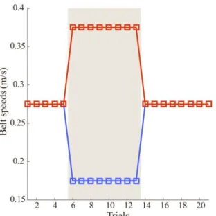
Every learning session relied on a sequence of baseline (tied-belt), adaptation (split-belt), and post-adaptation (tied-belt) trials. Each trial lasted for 60s, with short periods of rest in between each trial where the motors were turned off. During the tied-belt trials, the speed of the belts was set to 0.275m/s. During the split-belt trials the speed of the fast limb was set to 0.375m/s and the slow limb was set to 0.175m/s (a ratio of 2.14:1).

Two types of protocols were performed: short (1-day duration) and long (5-day duration). The short protocol was done for the Thy1-ChR2-YFP and VGlut2-ChR2-YFP manipulations, where a control session consisting of 21 trials (schematic found in Figure 2.4) was followed by an optogenetical stimulation protocol consisting of 27 trials, 21 of which were stimulated trials following the same schematic as the controls. The extra 6 trials were non-stimulated with three at behavior. The AAVretro-Jaws animals performed the long protocol, with both the control and stimulation sessions having a total of 54 trials over the duration of 5 days (schematic found in Figure 2.5 dashed lines represent the division of the days). However, the first and last three trials of the protocol were non-stimulated trials. The black bar in Figure 2.5 represents the trials when the laser was turned on.

Figure 2.4 Short protocol performed in the Split-belt treadmill for the Thy1-ChR2-YFP and VGlut2-ChR2-YFP manipulations. Red refers to the fast paw (0.375 m/s) and blue to the slow paw (0.175 m/s). The grey patch indicates which trials were done with the split-configuration. For the controls (N = 21 trials), the session consisted of 5 initial baseline trials, followed by 8 split, and finishing with 8 post-adaptation tied trials. For the stimulations (N = 27 trials), we followed the same speed protocol where all 21 trials were stimulated and added three non-stimulated trials at the start and end of the session.

Figure 2.5 Long protocol performed in the Split-belt treadmill for the AAVretro-Jaws manipulation. Red refers to the fast paw (0.375 m/s) and blue to the slow paw (0.175 m/s). The grey patch indicates which trials were done with the split configuration. A total of 54 trials were performed for both the control and stimulation sessions, over the course of 5 days. For both conditions, the protocol consisted of 12 initial baseline trials, followed by 22 split, and finishing with 20 post-adaptation trials. The dashed lines represent the division of the days. The black bar on top indicates in which trials the laser was turned on, with a total of 48 stimulated trials.

2.1.6. Laser stimulation protocols

For the Thy1-ChR2-YFP manipulation we applied three stimulation protocols: 2Hz right limb fast (2Hz RF), 10Hz right limb fast (10Hz RF) and 10Hz left limb fast (10Hz LF). The laser power was adjusted for each animal before the session began, with a slight paw tremor as our desired phenotype. The used laser powers are in the list below:

2Hz RF: (0.54 0.42)mW with a duty cycle of 20% (N=9); 10Hz RF: (0.67 0.47)mW with a duty cycle of 20% (N=9); 10Hz LF: (0.53 0.35)mW with a duty cycle of 20% (N=6).

For the VGlut2-ChR2-YFP manipulation we only performed one stimulation protocol: 10Hz right limb fast (10Hz RF). As our desired phenotype was the same as the Thy1-ChR2-YFP manipulation, the laser power was adjusted for each animal. The used laser power was (2.4 0.85)mW with a duty cycle of 20% (N=2). Finally, for the AAVretro-Jaws manipulation, as this refereed to an inhibition of climbing fiber activity, we used a laser power was 20mW with a duty cycle of 50% for all of the animals (N=3).

2.1.7. Data analysis

A symmetry analysis was performed on the four locomotion parameters (see section 2.1.4) by subtracting the parameter values of the slow front limb from the fast front limb (e.g., front symmetry=front fast-front slow). In this thesis, we focused only on the front limbs since these are those that have been shown to learn more clearly [2]. Later, an animal average for each trial was computed. Before plotting any of the calculated parameters, we performed a baseline subtraction by computing the mean initial baseline and subtracting its value for each trial. In both short and long protocols, the control baseline was taken from the initial tied trials prior to the splitting of the belts (trial 1 to 5 for the short; trial 1 to 12 for the long). Regarding the stimulation baseline, we considered only the initial baseline trials where the laser was turned on (trial 4 to 8 for the short; trial 4 to 12 for the long).

We performed a statistical analysis for all three manipulations using MATLAB. We used the mean of the first two trials of the post-adaptation phase to serve as a quantifiable measure of learning (aftereffect) and compared control and stimulation sessions via paired t-tests. Adaptation slopes were calculated by fitting a linear regression model to all split data points in both average and individual animal data. A comparison between sessions was performed via paired t-test. We used a significance cutoff of 0.05 for all statistics, with statistical significance indicated in the plots by * for p < 0.05.

2.1.8. Histology

After the stimulation sessions, animals were perfused with 4% paraformaldehyde and their brains removed, to examine the position of the implanted optical fiber. Coronal and sagittal sections were cut in a vibratome and mounted on glass slides with moiol mounting medium. All histology results were acquired via a confocal laser point-scanning microscope (Zeiss LSM 710), using a 10x objective. For the histology of the Thy1-ChR2-YFP animals, a 20x objective was also used to observe the axonal projections to the inferior olive.

2.2. Imaging

In this work we used a calcium imaging technique to image climbing fiber activity. We combined wide-field microscopy with activity-dependent fluorescence labelling to observe the complex spike activity in Purkinje cell dendrites. As calcium (Ca2+_{) is involved in neurotransmitter release, with the} aid of calcium fluorescent markers we may perform optical measurements and estimate its concentration in these cells [39] [42]. This allows us to record neuronal activity in living tissue in vivo.

We implemented an ultra-sensitive protein calcium sensor named GCaMP6f that emits fluorescence transients in the neurons in the presence of a blue light-source. With a cranial window placed above the cerebellar cortex we could observe the activity of the Purkinje cells after expression of the calcium sensor. The mouse was head-fixed and allowed to walk on top of a self-paced rotary treadmill. In this section we explore the methods related to the construction of the setup, the alterations to the tracking algorithm, and the imaging processing pipeline used to identify and extract individual cell activity.

2.2.1. Surgical procedures

Animals of C57BL/6 (wild type) line were anesthetized with isoflurane and placed in a stereotaxic frame (David Kopf Instruments, Tujunga, CA). Three hours before the surgery began, dexamethasone (0.1mg/kg) was administered to reduce swelling during and after the procedure. A 3mm cranial window was made on the right side of the skull, beneath lambda, the meeting point of the sagittal and the lambdoid suture, with the aid of a biopsy punch (Miltex GmbH). Three viral injections (315nl of volume each) of the AAV1.CAG.GCaMP6f.WPRE.SV40 (AV-1-PV3081 Upen) virus were made using Nanoject II (Drummond). During the injection, the DV coordinate injected volumes in each. A 3mm glass window was used to cover the craniotomy, being fixed into place by tissue adhesive (3M Vetbond). Finally, a head plate was fixed to the skull, near bregma, with the aid of dental cement (Super Bond, C&B). The rotary treadmill protocols began three weeks later to allow the virus to fully express, with continuous monitorization of any signs of pain or discomfort.

2.2.2. Experimental setup

We built a circular resin transparent treadmill with a diameter of 25cm and a width of 5cm. The setup was fixed to a horizontal pole passing through its center, allowing the treadmill to perform a circular motion around that axis. Two posts were positioned on the highest point of the treadmill, slightly angled to the front, so that the head of the mouse would be fixed. A corridor with transparent walls, black removable roof and a sliding door was placed behind the head-fixing posts. This corridor allowed the head fixing procedure to be performed in a much smoother fashion for both the mouse and the experimenter. A mirror was placed underneath and behind the head-fixing posts, with an 45 allowing a high-resolution camera (Pike F-032 B/C, Allied Vision Technologies) to acquire movies at 330 fps of the mice walking on top of the rotary treadmill. Six LED matrix infrared lights were positioned below the treadmill and angled towards the top, so the best lighting and contrast could be achieved. We used a one-photon microscope equipped with three linear stages that allowed to accurately position it across three dimensions. A 4x lens (Misumi) was used in our recordings, with a camera recording the images with a frame rate of 30 fps. An

Figure 2.6 Rotary treadmill experimental setup. A circular resin transparent treadmill with a diameter of 25cm and a width of 7cm was fixed to a horizontal pole passing through its center, allowing a circular motion to performed around that axis. Two posts were positioned on the highest point of the treadmill, slightly angled to the front, so that the head of the mouse would be fixed. A corridor with transparent walls, black removable roof and a sliding door was placed behind the head-fixing posts, allowing the head fixing procedure to be performed in a much smoother fashion for both the mouse and the experimenter. A high-resolution camera was used to acquire movies at 330 fps of the mice walking on top of the rotary treadmill. LED matrix infrared lights were positioned below the treadmill and angled towards the top, so the best lighting and contrast could be achieved. A 4x microscopy lens was used in our recordings, equipped with a camera recording the images with a frame rate of 30 fps.

2.2.3. Experimental protocols

A week of daily training sessions began two weeks after the surgical procedure. These sessions had the main objective of habituating the animals to be head-fixed and to run on top of the rotary treadmill with no need of the experimenter to intervene. Once full expression of the virus was achieved, we recorded testing videos for further analysis.

2.2.4. Rotary treadmill tracking algorithm

We modified the LocoMouse tracking algorithm, to allow tracking of the four paws on the rotary treadmill

boundary box was implemented. We also changed the shape of the original paw filter (described in [2]) by using a Gaussian function with a 5mm standard deviation.

2.2.5. Imaging analysis

Each testing video captured during the experimental sessions went through a pre-processing phase involving a movement correction algorithm ([43]). After the necessary frame alignment, an automated algorithm involving PCA and ICA procedures was performed to automatically identify Purkinje cells dendrites and retrieve complex spike activity. When viewed from the top, these Purkinje cell dendrites have an elongated shape and appeared parallel to each other. Each step of the algorithm is described in the diagram (Figure 2.7) and text below. This subsection of the

methods relies strongly on the paper by Mukamel ([29]), with some alterations made by us. Mukamel viewed Purkinje cell activity, retrieving individual cells in the surface of the cerebellum with a shape similar to lines parallel to each other, as it is expected from Purkinje cell dendrites.

The first step of the Mukamel algorithm consists in applying Principal Component Analysis (PCA), to exclude noise sources via reduction of the dimensionality of the data. By calculating the temporal covariance matrix, which allows us to treat large data sets, we compute both the spatial filter and the time course matrix that defines each principal component (PC). Then, we remove a selection of five PCs with the largest eigenvalues, to exclude noise sources with high variability.

A noise threshold was also set by creating a reference movie with the same dimensions as the recorded trials, but with independent Gaussian distributed random noise. By comparing the variance spectrum of the reference movie to the data, we determine which PCs were above the threshold and include them in the final selection [44]. Figure 2.8 illustrates an example of the referred selection process.

However, PCA cannot isolate individual cells. As this process relies on variance differences to define its components, certain cells with similar activity are included in the same component. Therefore, the gathered PCs generally had a mixture of signals from a variety of different cells. To successfully separate these signals, the algorithm applies Independent Component Analysis (ICA). This process extracts the signals from each cell, by searching for pairs of spatial filters and time traces that are sparse and statistically independent from one another. To study both the spatial and temporal sparseness, the Mukamel algorithm uses spatio-temporal ICA (stICA). Generally, spatial ICA gathers more accurate results in our data sets, being the process used in this thesis project.

Figure 2.7 Mukamel cell sorting algorithm divided into five stages ([29]). Firstly, principal component analysis is performed to reduce noise sources via dimensional reduction. The second step relies on gathering individual components, each of which referring to intracellular Ca2+ _{signals. With these, an image segmentation procedure is implemented to separate}

Figure 2.8 Example of the selection process applied to the gathered PCs. We generally exclude the first 5 PCs with the highest eigenvalues to remove noise sources with high variability. Then, with the aid of a noise threshold, we choose the PCs that are above the said threshold. In this example we selected 400 PCs.

Following the application of ICA, a third step of image segmentation is implemented, due to some ICs representing more than one cell. The first phase of this segmentation process consists in a smoothing of the filters via convolution with a Gaussian

pixels). After this, a threshold of 1.5 standard deviations above the mean is applied to obtain a binary mask. Every mask with a size below 50 pixels is then excluded from further analysis. This was done to reassure that no artifacts were confounding our results and just the cells were being selected. Finally, every pixel inside the selected area had their weights equal to the original filter, with the pixels outside the area set with weight equal to zero. The parameter values that are represented were chosen by us after an initial examination of our field-of-view and a manual selection of some ROIs, with later extraction of its area.

We also implemented an additional setup to

any irregular shaped ROIs. This ROIs were due to the presence of artifacts at the edges of the movie, blood vessels, or traces of cement from the surgical procedure. To solve this problem, we excluded ROIs using three distinct methods:

Centroid coordinates: We determine the centroid of each ROI and extract its coordinates via MATLAB function regionprops. Whenever the coordinates are close to the edges of the movies, we exclude the ROI, as it only represents image artificats resultant from the capture of the movie.

Ratio between major and minor axes: We determine the major and minor axes for each ROI (via MATLAB function regionprops) and calculated the ratio between both. Once a ROI showed a ratio with a value approximate to one, we assume a circular shape and excluded the cell from further analysis.

Boundary analysis: We applied a simple PCA analysis to each ROI using the MATLAB function pca. With this application we reduce the 2D boundary to a 1D trace. This trace gets smoothed via MATLAB function smooth and compared with the original by analysis of the correlation coefficient (via MATLAB function corrcoef). Once a ROI presents a coefficient below 0.99, we assume irregular shape and exclude it.

After this shape-based exclusion, the extraction of the signals from each cell can be finally performed. This is done by averaging the intensity over all the pixels inside the ROI for each time frame. Then, by removing the background intensity from all pixels in each frame and dividing by the same background, we retrieve the signal for the specific cell being analysed in units of F/F. With all the gathered signals, we calculate the frequency from the cell by counting the number of spikes based on an intensity threshold of 0.35 above the zero mean also used in the Mukamel paper.

3.

As this thesis work focuses on two distinct types of results, this chapter is divided into two sections, just as in Section 2: locomotor learning and imaging results.

3.1. Locomotor learning

This section presents results of the three optogenetical manipulations attempted to perturb climbing fiber activity.

3.1.1. Thy1-ChR2

Transgenic Thy1-ChR2-YFP mice performed four experimental sessions as schematized in Figure 2.4. The first was the control session (right-belt fast) without laser stimulation, followed by three stimulation sessions: 2Hz right-belt fast (2Hz RF), 10Hz right-belt fast (10Hz RF) and 10Hz left-belt fast (10Hz LF). For a better visualization of the results, we aligned all data to the first split-belt trial. Furthermore, only the stimulated trials from the three stimulation sessions are shown (trial 4 to 24), with a later analysis being shown focusing on the effects of laser activation on the baseline.

In our first experiment, we stimulate with double the spontaneous frequency expected from the climbing fibers (2Hz RF Figure 3.1 N = 9, both female and male). We expect this stimulation to not disrupt the normal performance on the setup, as the frequency is similar to the once expected from these cells, allowing them to maintain their ability to send their error signals throughout the session. Regarding the interlimb parameters (Figure 3.1a-c), animals show typical adaptation and post-adaptation curves, with a clear initial error and negative aftereffect in both protocols. We analyse two distinct features when studying these parameters: adaptation slope and aftereffect values. From our experience in the lab, a positive adaptation slope is not sufficient to see whether the animals learned or not, as certain animals may present flat adaptation curves yet still present an aftereffect. Thus, we use the aftereffect as a quantifiable measure of learning and the adaptation slope as an additional analysis to show expression of learning.

A linear regression model estimates the slope of the adaptation phase in both protocols (control slopes: mstep_length;control = 0.22, mdouble_support;control = 0.41, mcenter_of_oscillation;control = 0.14; 2Hz slopes: mstep_length;2HzRF = 0.44, mdouble_support;2HzRF = 0.56, mcenter_of_oscillation;2HzRF = 0.22). In all three parameters we observe an increase in the slopes when we performed the 2Hz RF protocol, yet we do not note statistical significance when comparing both protocols (control vs 2Hz RF adaptation slope: t8 = -1.46, p = 0.18; t8 = -0.87, p = 0.41; t8 = -1.28, p = 0.24; for step length, double support and center of oscillation symmetries respectively). With respect to the aftereffect, we do not show statistical significance when comparing protocols (control vs 2Hz RF aftereffect: t8 = 1.29, p = 0.23; t8 = 1.29, p = 0.23; t8 = 0.99, p = 0.35; for step length, double support and center of oscillation symmetries respectively). These results show that animals performed the task in a similar way as they did in the control protocol, with no effects from the stimulation being observed.

We then present the stride length symmetry (Figure 3.1d) that serves as a proxy of how well the animals walked during the sessions. The absence of a difference between protocols (control vs 2Hz RF) suggests a normal walking pattern during the laser manipulation. Our results show the typical

intralimb behaviour consisting of a rapid asymmetry once animals enter the split-trials that remains unaltered during this period, followed by a return to the normal baseline once the post-adaptation phase initiates. This was consistent in both the control and the 2Hz RF data, with no observable difference between both.

We can additionally observe the location of the optical fiber that was implanted in the histology results shown in Figure 3.1e. The fiber is located immediately above the left side of the inferior olive, with an additional amplified image in Figure 3.1f showing the projections that we are aiming to target with this manipulation.

Figure 3.1 Control vs 2H RF stimulation in Thy1-ChR2-YFP transgenic mice. All data points were aligned to the first split-belt trial of the stimulation session for a better comparison between protocols. The grey patch indicates the adaptation phase (split-trials). Only the stimulated trials (4 to 24) are represented. Black represents the control data and pink the stimulation data. For all three interlimb parameters, the aftereffect values from both protocols are represented, with statistical significance being shown (n.s no statistical significance). A: Step length symmetry (mm); B: Double support symmetry (%); C: Center of oscillation symmetry (mm). In all interlimb parameter plots, no statistical difference in the aftereffects is noted, with an increase in the adaptation slopes; D: Stride length symmetry (mm). No observable differences were noted between both protocols; E: Histology retrieved from one of the animals. Red represents calbindin, a calcium binding protein. Yellow represents cells that express channelrhodopsin-2 ion gate channel, marked with yellow fluorescent protein. The inferior olive is marked with dashed

In our second experiment, we aim to use the same animals as before while stimulating with ten times the spontaneous climbing fiber activity (10Hz RF Figure 3.2). When we stimulate with such a high frequency, we expect to perturb the normal functionality of the climbing fibers as they lose their ability to time their error signals whenever necessary.

Certain differences between both protocols can be observed in the interlimb parameters (Figure 3.2a-c). A smaller after effect and a somewhat flat adaptation curve are main features when analysing the step length and center of oscillation symmetries. The adaptation slopes were estimated using the same linear regression model as before (10Hz slopes: mstep_length;10Hz = 0.02, mdouble_support;10Hz = 0.28, mcenter_of_oscillation;10Hz = -0.03). In all three parameters the slope decreased its value, mainly in the step length and center of oscillation symmetries, but no statistical difference between the protocols is observed (control vs 10Hz RF adaptation slopes: t8 = 1.42, p = 0.19; t8 = 0.54, p = 0.60; t8 = 2.09, p = 0.07; for step length, double support and center of oscillation symmetries respectively). Our analysis of the aftereffect shows a clear decrease in the step length and center of oscillation parameters, but no observable difference in the double support. Statistically, no significant difference was shown in the double support and center of oscillation, with a significant difference when analysing the step length (control vs 10Hz RF aftereffect: t8 = 3.16, p = 0.01; t8 = 1.11, p = 0.30; t8 = 1.95, p = 0.09; for step length, double support and center of oscillation symmetries respectively). These results suggest that 10Hz stimulation impairs learning of step length symmetry.

Regarding the stride length symmetry (Figure 3.2d), our results show no differences when

comparing ility

Figure 3.2 Control vs 10HzRF stimulation in Thy1-ChR2-YFP transgenic mice. All data points were aligned to the first split-belt trial of the stimulation session for a better comparison between both protocols. The grey patch indicates the adaptation phase (split-trials). Only the stimulated trials (4 to 24) are represented. Black represents the control data and yellow the stimulation data. For all three interlimb parameters, the aftereffect values from both protocols are represented, with statistical significance being shown (n.s no statistical significance; * statistical significance with p < 0.05). A: Step length symmetry (mm). Statistical difference in the aftereffect values between both protocols. A decrease in the slope was noted when laser was turned on ; B: Double support symmetry (%). No statistical difference in the aftereffects between both protocols, with also a slight decrease in the slope of the adaptation phase; C: Center of oscillation symmetry (mm). No statistical difference in the aftereffects between both protocols, with a flat adaptation phase; D: Stride length symmetry (mm). No observable differences between both protocols.

After our analysis in the 10Hz RF experiment, we asked whether this effect in learning was specific when the contralateral side of the body was exposed to the fast belt. To answer this question, we performed the same stimulation protocol, but with the left side of the body going faster (10Hz LF Figure 3.3). With the fiber being placed above the left side of the inferior olive, we expect no effect on the normal animal behavior once we perturb the left-side of the body, since the climbing fibers project contralaterally to the cerebellar cortex. As in this case we have the left-side going faster, the symmetry analysis would present a negative learning curve. For a better visualization of the data and an easier comparison with the control protocol, we flipped the curves relative to the x-axis.

We only used six animals in this protocol from the original group, for some of them presented unwillingness to perform on the setup in the later sessions, not allowing more data collection. With this in mind, the control data only considers the six animals used in the 10Hz LF protocol. Regarding the interlimb parameters (Figure 3.3a-c), the same linear regression model estimates the adaptation slopes (control slopes: mstep_length;control;6 = 0.20, mdouble_support;control;6 = 0.27, mcenter_of_oscillation;control;6 = 0.15; 10Hz LF slopes: mstep_length;10HzLF = 0.45, mdouble_support;10HzLF = 0.48, mcenter_of_oscillation;10HzLF = 0.17). As we observed in the 2Hz RF study (see Figure 3.1), the adaptation

both protocols in all three interlimb parameters (control vs 10Hz LF adaptation slopes: t5 = 3.59, p = 0.02; t5 = 4.23, p = 0.01; t5 = 3.12, p = 0.03; for step length, double support and center of oscillation symmetries respectively . When analysing the after effects, no significant difference when comparing the two protocols is shown (control vs 10Hz LF aftereffect: t5 = 1.02, p = 0.26; t5 = 0.27, p = 0.80; t5 = 0.99, p = 0.37; for step length, double support and center of oscillation symmetries respectively), indicating that the animals learned just as they did in the control session. We extended our analysis to the stride length symmetry (Figure 3.3d), where we observe some variability during the split trials, the typical intralimb behavior is still evident. The existing noise that we observe might explain certain changes in the other three parameters, as the walking pattern of the animals affects the coordination between the limbs.

Figure 3.3 Control vs 10HzLF stimulation in Thy1-ChR2-YFP transgenic mice. All data points were aligned to the first split-belt trial of the stimulation session for a better comparison between both protocols. The grey patch indicates the adaptation phase (split-trials). Only the stimulated trials (4 to 24) are represented. Black represents the control data and blue the stimulation data. For all three interlimb parameters, the aftereffect values from both protocols are represented, with statistical significance being shown (n.s no statistical significance). A: Step length symmetry (mm); B: Double support symmetry (%); C: Center of oscillation symmetry (mm). No statistical difference in the aftereffects between both protocols. When comparing the adaptation slopes from both protocols, we observe an increase in the slopes for all three parameters for the stimulation protocol. Statistical significance was evident in all three interlimb parameters. D: Stride length symmetry (mm). We note some variability throughout the adaptation phase that can explain value jumps in the three interlimb parameters. Despite this variability, the normal intralimb behavior is visible in both protocols

After our analysis of all three stimulation protocols, we asked ourselves what was the impact that the laser had on the normal baseline behavior of the animal. Figure 3.4 shows the five initial baseline trials for all four protocols color coded as above. As the 10Hz LF protocol had less animals in its experimental population, we only selected the animals that matched the ones in that protocol. We immediately observe an animal in the 10Hz RF protocol that has a trial with a high asymmetry during the baseline phase in the step length and center of oscillation symmetries. As this behavior did not appear on the other protocols, we account this outlier as an irregularity from the behavior of the animal on that specific trial, probably due to improper walking.

We note an increase in the step length and center of oscillation baselines and a decrease when analysing the double support. These shifts seem to be consistent for the high frequency protocols, yet the 2Hz RF does not show the same effect, being similar when compared with the control. These results suggest a perturbation in the normal locomotion of the animal by creating an initial asymmetry in the walking pattern already during the tied-belt trials. In attempt to understand this result, we need to observe the histology results in Figure 3.1e,f. The projections to the inferior olive are expressing channelrhodopsin-2, but this expression also targets several brain stem structures surrounding the fiber. We have achieved an anatomical specific perturbation of the projections to the inferior olive, but with a lack of genetic specificity. Our next goal is to focus on additional experiments to achieve both anatomic and genetic specificity.

Figure 3.4 Baseline analysis between the control and stimulation protocols in the Thy1-ChR2-YFP transgenic mice. Individual animals are represented with dashed lines and the average acoss animals with the thick line. The five initial baseline trials were chosen from the control data, with the five stimulated baseline trials being chosen from the stimulation protocols. As the 10Hz LF protocol has a smaller experimental population, we matched the animals from the other protocols, only presenting a total of six animals in this data. An individual animal showed high asymmetry in one trial during the 10Hz RF protocol. As this effect was not evident in the rest of the protocols, we conclude that this was due to irregularity in the anim behavior in that specific trial. The highest frequency protocols show an increase in the baseline in the step length and center of oscillation and a decrease in the double support. This was not evident in the 2Hz RF protocol, that showed great similarity with the control baseline.