Visualizations of Boger Fluid Flows in a 4:1
Square–Square Contraction
M. A. Alves
Depto. de Engenharia Quı´mica, CEFT, Faculdade de Engenharia da Universidade do Porto, 4200-465 Porto, Portugal
F. T. Pinho
Centro de Estudos de Feno´menos de Transporte, Depto. de Engenharia Mecaˆnica, Universidade do Minho, Campus de Azure´m, 4800-058 Guimara˜es, Portugal
P. J. Oliveira
Depto. de Engenharia Electromecaˆnica, Unidade Materiais Teˆxteis e Papeleiros, Universidade da Beira Interior, 6201-001 Covilha˜, Portugal
DOI 10.1002/aic.10555
Published online August 12, 2005 in Wiley InterScience (www.interscience.wiley.com).
Visualizations of the 3-D flow in a 4:1 square–square sudden contraction for two viscoelastic Boger fluids and two Newtonian fluids were carried out at low Reynolds numbers. In these creeping flow conditions, the vortex length remained unchanged for Newtonian fluids, whereas a nonmonotonic variation with flow rate was observed for the Boger fluids. Initially, the corner vortex slightly increased with flow rate to a local peak at a Deborah number of De2⬇ 6, before decreasing significantly to a minimum at De2⬇
15 (De2is based on downstream characteristics). Finally, for Deborah numbers⬎ 20
there was intense vortex enhancement until a periodic flow was established at higher flow rates (De2 ⬇ 45–52). The strong elastic vortex enhancement was preceded by the
appearance of diverging streamlines on the approach flow and, for the Boger fluid with higher polymer concentration, vortex enhancement took place through a lip vortex mechanism.© 2005 American Institute of Chemical Engineers AIChE J, 51: 2908 –2922, 2005
Keywords: viscoelastic flow, Boger fluid, diverging flow, visualization, 3D contraction flow
Introduction
Flow visualizations have always been important in fluid mechanics and motivated a wealth of research in the field, as illustrated in Van Dyke’s classic work An Album of Fluid Motion.1They provide a clear insight of many phenomena and
reinforce elaborate mathematics. Non-Newtonian fluids are usually more viscous than common Newtonian fluids and their flows are frequently investigated by flow visualization because
they tend to take place in the laminar regime. A compilation of flow visualization studies specifically for non-Newtonian flu-ids, was written by Boger and Walters in 1993,2and constitutes
a representative sample of works published in this important subfield of fluid mechanics.
Sudden contraction flows are classical benchmark problems used in computational rheology,3with the explicit assumption
of two-dimensional (2-D) flow to simplify the simulations, and a large number of visualization studies in planar and axisym-metric contractions have been published in the literature. The flow behavior of non-Newtonian fluids in these simple config-urations can be very surprising; there can be substantially different flow patterns for fluids with apparently similar Correspondence concerning this article should be addressed to M. A. Alves at
rheological characteristics, and distinct patterns also arise in comparable configurations as a result of geometric differences (such as planar vs. axisymmetric).
The following paragraphs provide a review of relevant works in sudden contraction flows of axisymmetric, planar, and square–square type, and a summary of the main conclusions is presented in Table 1.
Axisymmetric contractions
For axisymmetric contractions, pioneering visualization studies with viscoelastic fluids were carried out by Cable and Boger4-6and Nguyen and Boger,7who also reviewed previous
work in the field. At low flow rates they observed that the salient corner vortex was controlled by viscous forces and a normalized length of 0.18 was measured, with the normaliza-tion based on the upstream pipe diameter. At higher flow rates a dramatic vortex growth was reported for all geometries (cf. Table 1) and for both shear-thinning and constant viscosity elastic fluids. At even higher Deborah numbers the flow be-came asymmetric and time dependent. At intermediate condi-tions Cable and Boger observed the onset of diverging flow upstream of the contraction plane and the simultaneous reduc-tion of the salient vortex length, a phenomenon partially attrib-uted to inertia. Fluid elasticity was considered the cause for the flow instabilities because the Reynolds numbers were well below those associated with transitions arising from inertial effects.
From the mid-1980s the 4:1 contraction became the focus of a variety of experimental and numerical work. The experimen-tal work concentrated on the investigation of low Reynolds number flow transitions and elastic instabilities and relied on several techniques, as in McKinley et al.8 At that time the
numerical methods were usually unable to predict accurately the subcritical steady flows and the emphasis was focused on improving the numerical techniques.
In 1986 Boger et al.9 investigated the behavior of two
different Boger fluids having similar shear properties and yet found quite different vortex dynamics; for a polyisobutylene in polybutene fluid (PIB/PB) vortex enhancement was preceded by the growth of a lip vortex, whereas for polyacrylamide dissolved in corner syrup (PAA/CS) the lip vortex was absent. It was concluded that an additional measure of extensional properties had to be taken into account and in his 1987 review paper10Boger suggested that parameter to be the extensional
viscosity, and described in more detail the flow dynamics in the sudden contraction with increasing Deborah number. For some fluids only a convex corner vortex exists, growing in size and becoming concave as elasticity increases. For other fluids the corner vortex extends to the reentrant corner, and a lip vortex is formed. For high contraction ratios, the two vortices are initially separated, but similar distinct vortices were also seen by McKinley et al.8in small contraction-ratio experiments. As
the elasticity increases, the strength of the lip vortex grows at the expense of the corner vortex, whereas the length of the latter remains unchanged. Eventually, the lip vortex occupies the whole contraction plane region and a further increase in the Deborah number leads to a larger concave-shaped vortex. At even higher Deborah numbers a small pulsating lip vortex now appears and leads to unsteady behavior. All these features have
been observed in axisymmetric contractions under conditions of negligible inertia.
Recent experimental investigations by Rothstein and Mc-Kinley11,12 clearly demonstrate the important role of
exten-sional viscosity on the dynamics of vortex growth and on the associated enhanced pressure drop in contraction flows. They conjectured that the extra pressure drop results from an extra dissipative contribution to the elastic stress arising from a stress-conformation hysteresis in the nonhomogeneous exten-sional flow generated near the contraction plane. Such conjec-ture has implications on constitutive-equation modeling and led to the recent numerical simulations of Phillips et al.13with a
closed form of the adaptive length scale (ALS) model of Ghosh et al.,14 which accounts for hysteresis of the conformation
tensor. These authors were able to qualitatively predict large pressure drop enhancements, although there were still discrep-ancies in comparison with experiments.
Planar contractions
Investigations in planar contraction flows began soon after those in axisymmetric contractions and, although they con-firmed some of the findings observed for the circular geome-tries, some notable discrepancies also emerged. Walters and Webster15found no significant vortex activity for Boger fluids
in the 4:1 case, in marked contrast to observations in 4.4:1 circular contractions. However, for shear-thinning fluids vortex growth was observed in both planar and axisymmetric geom-etries. To help clarify these differences, Evans and Walters16
studied the flows of shear-thinning and constant viscosity elas-tic fluids (aqueous solutions of polyacrylamide) through planar contractions (contraction ratios of 4:1, 16:1, and 80:1) and always found strong vortex enhancement for the shear-thinning fluids, even for the smaller contraction ratio, and difficulties in observing vortex activity for Boger fluids. They also reported that both the contraction ratio and fluid elasticity contributed to vortex enhancement with shear-thinning fluids. However, for the larger contraction ratios a lip vortex was seen and a growth mechanism similar to that previously found for circular dies was observed, although in the 4:1 planar contraction there was no sign of such a lip vortex. In a subsequent paper Evans and Walters17looked at the behavior of shear-thinning fluids in the
smaller contraction ratio of 4:1 to investigate whether a lip vortex mechanism of vortex growth was still at work. They found that for the less viscous/concentrated polymer solutions such lip vortex could be generated and that inertia played a critical role in separating the corner and lip vortices. Indepen-dent lip and corner vortices were also found in the numerical simulations of creeping flow by Alves et al.18,19 for a 4:1
contraction with Boger fluids represented by either the upper convected Maxwell (UCM) or the Oldroyd-B models.
The relevance of extensional viscosity in planar contraction flows was emphasized in the experimental investigations of White and Baird,20,21who used two polymer melts: polystyrene
(PS) and low-density polyethylene (LDPE). Whereas a vortex was observed for the LDPE, it was absent from PS flows and the difference was attributed to the distinct extensional viscos-ities, given their similar weak shear-thinning behavior. This was corroborated when the same authors later used a constitu-tive equation that represented accurately the measured exten-sional viscosity of both fluids,22 and were able to predict
Table 1. Relevant Investigations of Viscoelastic Fluid Flow in Axisymmetric, Planar, and Square Contractions*
Ref. Authors (year)
Flow Conditions and Test
Fluids Main Conclusions
4–6 Cable and Boger (1978, 1979)
Circular, ⫽ 2, 4 Shear-thinning fluids
Vortex flow regime with vortex growth at low flow rates. Divergent flow regime at intermediate flow rates and
inertial effects.
Unstable flow regime at large flow rates. 7 Nguyen and Boger
(1979)
Circular, 4⬍ ⬍ 14.6 Boger and shear-thinning
fluids
Sequence of flow regimes referring to lip vortex behavior:
(1) vortex growth; (2) asymmetric flow; (3) rotating flow; (4) helical flow (pulsating).
15 Walters and Webster (1982)
Planar and circular, ⫽ 4 Boger and shear-thinning
fluids
Boger fluids: substantial vortex activity in circular contraction and virtually none in planar case. Shear-thinning fluid: substantial vortex activity in circular
and planar contractions.
Rounding the corner dramatically changes flow. 24 Walters and Rawlinson
(1982)
Planar, ⫽ 13.3 SQ/SQ, ⫽ 13.3 Boger fluids
No noticeable vortex activity for the 13.3:1 planar contraction.
Significant vortices observed for the 13.3:1 3-D SQ/SQ contraction.
Vortex enhancement with increasing flow rate. Slight asymmetry at highest flow rates. 9 Boger et al. (1986) Circular, 4.4⬍ ⬍ 16.5
Boger fluids
Simultaneous lip and corner vortices, with lip vortex dominating as De increases:
De⬍ 3 no influence of on lip vortex; De⬎ 3 influence of on lip vortex. 16 Evans and Walters
(1986)
Planar, ⫽ 4, 16, 80 Boger and shear-thinning
fluids SQ/SQ, ⫽ 16 Boger fluids
Planar:
Boger fluids: difficulty in observing vortex activity. Shear-thinning fluids: substantial vortex activity in all
cases.
Large: vortex growth associated with lip vortex. Small: vortex growth is not associated with lip
vortex. SQ/SQ:
Strong vortex enhancement for Boger fluids. 20 White and Baird
(1986)
Planar, ⫽ 5.9 Weakly shear-thinning
melts
Vortex growth for LDPE due to early onset of shear-thinning and strain hardening extensional viscosity. No vortex growth for PS which has no strain hardening
extensional viscosity. Relevance of extensional viscosity. 21 White and Baird
(1988)
Planar, ⫽ 4, 8 Weakly shear thinning
polymer melts (LDPE, PS)
Confirmation of the observations of White and Baird20
for lower and higher contraction ratios.
22 White and Baird (1988)
Planar, ⫽ 4, 8 Numerical, Full PTT, ⫽
0
Simulations confirm experiments of White and Baird21in
terms of streamlines and birefringence.
Size and intensity of vortex determined by parameter, which controls extensional viscosity in the PTT model.
17 Evans and Walters (1989)
Planar, ⫽ 4 Shear-thinning fluids
For some fluids there are lip and corner vortices, with the former responsible for the vortex enhancement mechanisms, as for large.
For mobile fluids inertia separates corner and lip vortices. 8 McKinley et al. (1991) Circular, 2⬍ ⬍ 8
Boger fluid
Sequence of flow regimes near the lip vortex: (1) stable; (2) time periodic; (3) quasi-periodic; (4) aperiodic. Time-dependent 3-D flow for 2⬍ ⬍ 5 at high flow
rates.
Rounding corner delays transitions. 46 Boger and Binington
(1994)
Circular, ⫽ 4 Sharp and rounded
reentrant corner Boger fluids
Each of the two fluids studied react differently to the rounded corner: dramatic changes are observed for the polyacrylamide based Boger fluid, in deep contrast to less dramatic changes observed for the polyisobutylene based fluid.
47 Purnode and Crochet (1996)
Numerical simulations with a FENE-P model Planar, ⫽ 4, 16, 80 Shear-thinning fluids
Predictions qualitatively match the experimental results of Evans and Walters.16,17
Lip vortex not associated with inertia. 26 Mompean and Deville
(1997)
Numerical, Oldroyd-B model
2-D, ⫽ 4 3-D planar ⫽ 4
2-D: no prediction of lip vortex; decrease of corner vortex size with Deborah number.
3-D: Corner vortex in center plane always smaller than in 2D case.
numerically, at least qualitatively, the different vortex patterns observed.
The surprisingly different behavior of Boger fluids in circu-lar and planar contractions has been further studied by Nigen and Walters.23Experiments in both types of contraction were
conducted with Newtonian and Boger fluids having identical shear viscosities and it was demonstrated that, although there were higher extensional strain rates in the planar geometry than in the circular die, virtually no elastic vortex enhancement was found in the former geometry in contrast to the latter. Given that the vortex dynamics is a complex function of strain rates, strains, and molecular conformation histories,12 these
differ-ences are not so surprising. Square–square contractions
Experiments with flows through square–square contractions are scarce, partly because they are more complex but also because of their inadequacy to be used for comparison with 2-D simulations. In their 1982 experiments, Walters and Raw-linson24reported similarities between the flows through
circu-lar and square–square contractions. In particucircu-lar, the
differ-ences found between flows of Boger fluids in planar and circular contractions were also seen for planar and 13.3:1 square–square contractions and at intermediate Deborah num-bers a diverging flow was seen upstream of the contraction as originally observed by Cable and Boger4 for circular
geome-tries.
In the square duct contraction, and in contrast to the 2-D planar case, isopressure lines can close in the cross-stream directions, as in the axisymmetric geometry, but there are now normal stress imbalances leading to secondary flows. The dy-namics of the vortices in combination with these new second-ary flow structures and fluid elasticity are still to be well characterized and understood.
In view of the above, it comes as no surprise that flow predictions of square–square contraction flows are virtually inexistent except for the work of Xue et al.,25to be discussed
below. Most of the existing three-dimensional (3-D) viscoelas-tic flow simulations in contractions basically considered the 2-D planar contraction extending along the spanwise direction and so the 3-D effects were attributed only to the presence of end walls. Some computations of such planar 3-D contraction
Table 1. Relevant Investigations of Viscoelastic Fluid Flow in Axisymmetric, Planar, and Square Contractions* (Continued)
Ref. Authors (year)
Flow Conditions and Test
Fluids Main Conclusions
27 Xue et al. (1998) Numerical 2-D: UCM
3-D planar: Boger and shear-thinning fluids (UCM, PTT with ⫽ 0)
2-D: Lip and corner vortex growth mechanisms depending on elasticity and Deborah numbers. Appearance of lip vortex depends on polymer viscosity and is promoted by inertia. 3-D planar
䡠 UCM: confirms presence of lip vortex for some flow conditions.
䡠 PTT: qualitative agreement with experiments of Quinzani et al.48
25 Xue et al. (1998) Numerical
2D and 3D SQ/SQ, ⫽ 4 Boger and shear-thinning
fluids: UCM, PTT ( ⫽ 0)
Relevance of transient extensional behavior along centerline. In 3-D vortex activity correlates well with steady extensional properties, but not in 2-D.
11 Rothstein and McKinley (1999)
Circular, ⫽ 4 Boger fluid
Measurement of enhanced pressure drop. It is suggested that this is attributable to an additional dissipative contribution of polymer stress manifested in stress conformation hysteresis.
18 42 43
Oliveira and Pinho (1999); Alves et al. (2000)
Planar, numerical  ⫽ 4
UCM and PTT fluids
Lip vortex growth mechanism for UCM fluid. No lip vortex for PTT fluid.
Streamline divergence for high Deborah flows, enhanced by inertial effects (UCM).
Importance of mesh refinement and discretization schemes for numerical accuracy.
12 Rothstein and McKinley (2001) Circular, 2⬍ ⬍ 8 Various curvatures of corner Boger fluid
 ⫽ 2: steady elastic lip vortex
4ⱕ ⱕ 8: no lip vortex observed, only corner vortex. Rounding the reentrant corner leads to shifts in the onset
of flow transitions to larger Deborah numbers. The role of contraction ratio on vortex growth dynamics
is rationalized by using a dimensionless ratio of the elastic normal stress difference in steady shear flow to that in transient uniaxial extension.
23 Nigen and Walters (2002)
Planar and circular 2ⱕ ⱕ 32 Boger fluids
Planar case: no sign of steady vortex enhancement Circular: lip mechanism responsible for vortex growth
and enhanced pressure drop. 19 Alves et al. (2003) Planar, numerical; ⫽ 4
Highly refined mesh Oldroyd-B and PTT (linear and exponential) models
Lip vortex enhancement for Oldroyd-B fluid accompanied by decrease in corner vortex. Intense corner vortex growth for linear PTT and no lip
vortex.
High Deborah number simulations for PTT models.
flows (in fact, quasi-2-D) were presented by Mompean and Deville26and Xue et al.27; their intention was mainly to
illus-trate the capabilities of their finite-volume methods in 3-D simulations, so they did not comment on the results of their calculations in relation to 3-D effects and in fact the detailed 3-D flow structure was not well resolved. The only 3-D effect mentioned by Xue et al.27was that the average velocity in a
3-D channel differs from the average velocity in a 2-D channel, and therefore the Deborah number should be modified accord-ingly.
In a second article, Xue et al.25 tackled the actual 3-D
square–square contraction using the Phan-Thien–Tanner model (PTT) (with a nonzero second normal stress difference coeffi-cient) and UCM constitutive equations. They found strong vortex enhancement for both fluid models, in contrast to the results for the planar contraction where only the PTT fluid (shear-thinning fluid) exhibited vortex enhancement. These contrasting behaviors mirror those observed experimentally for axisymmetric and planar contraction flows, and are explained by the 3-D nature of circular and square–square contractions. The numerical investigations of Xue et al.25related the
calcu-lated flow dynamics with the transient extensional viscosity of the fluids, but nothing was reported regarding unexpected sec-ondary flows in the contraction region or the onset of flow instabilities; they did mention, however, the existence of the well-known secondary flow in the fully developed straight upstream and downstream noncircular ducts.
In conclusion, the vast majority of experimental work on contraction flows of viscoelastic liquids has been on axisym-metric and (approximately) planar configurations, with the expectation that 2-D numerical simulations would allow for adequate predictions. A square–square contraction arrange-ment is a good compromise between geometric simplicity and complex 3-D flow structure, and appears as a good candidate for a prototype 3-D test case that is necessary for validating numerical 3-D codes. However, before embarking on the heavy task of performing full 3-D simulations of such viscoelastic flows, both under steady and transient conditions, a thorough experimental investigation is required. This is the motivation for the present experimental work, which concentrates on char-acterizing the flow patterns in square–square contractions of elastic fluids having a constant shear viscosity.
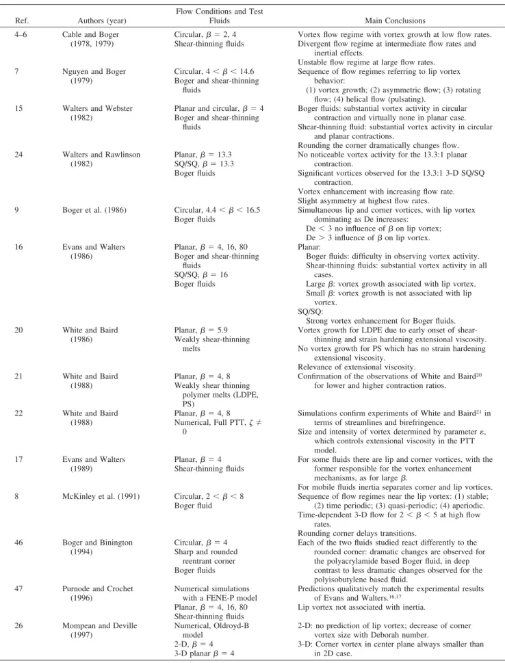
Experimental Setup
The experimental apparatus is depicted in Figure 1. The rig consisted of two consecutive square ducts (length: 1000 and 300 mm) and a vessel. The sides of the square ducts were 2H1
⫽ 24.0 mm and 2H2⫽ 6.0 mm, respectively, thus defining the
4:1 contraction ratio. The flow rate was set by an adequate control of applied pressure on the upper duct and frictional losses in the long coiled pipe (T in Figure 1) located between the smaller duct and the vessel, at the bottom of the rig. To achieve low flow rates the coiled pipe was 8 m long and had a diameter of 4 mm, whereas for higher flow rates the diameter of the coiled pipe was 6 mm. Applied pressure was kept between 0.5 and 4 bar, and the dashed lines in Figure 1 represent the pressurized air lines. This flow arrangement ad-equately controlled the flow rate without significant constric-tions, such as valves, that would eventually degrade the
poly-mer molecules. The flow rate was measured by a stopwatch and the passage of the liquid-free surface at two marks in the upper duct. In all tests the fluid temperature was measured and the fluid properties were taken from the rheometric master curves shown in the next section. To improve the quality of the visualizations the rig was placed inside a dark room.
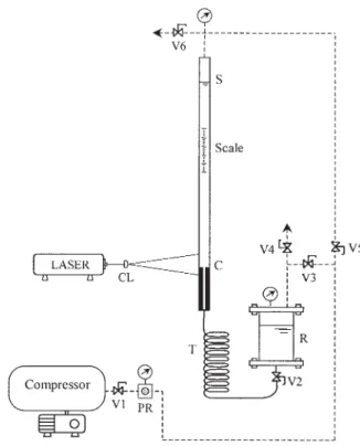
A 10 mW He–Ne laser light source was used to visualize the flow patterns. The laser beam passed through a cylindrical lens to generate a light sheet illuminating highly reflective tracer particles suspended in the fluid. These were 10 m PVC particles (at a concentration of about 15 mg/kg fluid) added during the preparation of the fluid. The path lines formed were recorded using long time exposure photography with a con-ventional camera (Canon EOS300 with a macro EF100 mm f/2.8 lens), as sketched in Figure 2, which includes a schematic representation of the test section. The terminal velocity of the PVC particles was negligible: assuming Stokes flow conditions it was estimated to be 0.15m/s in the less viscous Newtonian fluid used (N85), which is three orders of magnitude smaller than the minimum flow bulk velocity.
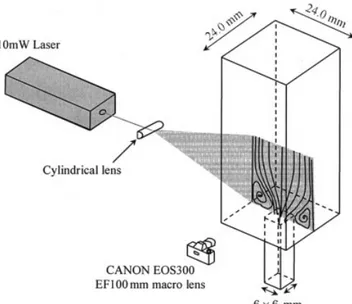
The shear viscosity () and the first normal stress difference coefficient (⌿1) in steady shear flow, and the storage and loss
moduli (G⬘, G⬙) in dynamic shear flow were used to charac-terize the rheology of the Boger fluids. These properties were measured with an AR2000 rheometer from TA Instruments, using a cone–plate setup with 40 mm diameter and 2° angle. A falling ball viscometer from Gilmont Instruments (model GV-2200) was also used for some viscosity measurements with the Newtonian fluid N85.
Figure 1. Flow rig.
PR, pressure regulator; V1 to V6, ball valves; R, reservoir; CL, cylindrical lens; T, long coiled pipe; S, free surface; C, contraction plane.
Rheological Characterization of the Fluids
Four fluids based on mixtures of glycerin and water were investigated: two viscous Newtonian fluids (N85 and N91) and two viscoelastic Boger fluids (PAA100 and PAA300). Their compositions, densities, and zero-shear rate viscosities are listed in Table 2. The Boger fluids were prepared by dissolving a small amount of polyacrylamide (PAA; Separan AP30 pro-duced by SNF Floerger) in the Newtonian solvent N91. To minimize the intensity of shear thinning a small amount of NaCl was added, as described in detail in Stokes.28To reduce
bacteriological degradation of the solutions the biocide Kathon LXE, produced by Rohm and Haas, was also added. The fluid densities were measured at 21.2°C using a picnometer. Newtonian fluids
For the N85 fluid the measured shear viscosity was ⫽ 0.125 Pa䡠s at 18°C, the temperature at which the visualizations took place. For the N91 fluid the rheometer was used to measure the shear viscosity at temperatures ranging from 15.9 to 25.0°C. This second Newtonian fluid, which served as solvent for the PAA solutions, was also used to evaluate the accuracy of the rheometer and to estimate the base noise level in dynamic tests (represented as the dashed baseline of 2G⬘ in Figures 3b and 4b). For N1, the measurements at␥˙ ⬍ 100 s⫺1
indicated a zero reading within experimental uncertainty, as they should. The uncertainty in measuring N1was of the order
of⫾10 Pa, in agreement with the specifications of the manu-facturer for the cone-plate geometry used. For␥˙ ⬎ 100 s⫺1
inertial effects became important, and negative values of N1
were measured. This inertial effect for Newtonian fluids was well predicted by the following equation29:
N1,inertia⫽ ⫺0.152R2 (1)
where and R represent the angular velocity and the radius of the cone, respectively.
The effect of temperature on the shear viscosity for the N91 fluid is well described by an Arrhenius equation, defining a shift factor aTof the form
ln共aT兲 ⫽ ln 共T兲 共T0兲 ⫽
冋
⌬H R冉
1 T⫺ 1 T0冊册
(2)Figure 2. Flow visualization technique and details of the test section.
Table 2. Composition and Properties of the Fluids (Mass Concentrations)
Designation PAA (ppm) Glycerin (%) Water (%) NaCl (%) Kathon (ppm) (kg/m3) 0(Pa䡠 s) N85 — 84.99 15.01 — 25 1221 0.125 (18°C) N91 — 90.99 7.51 1.50 25 1250 0.367 (20°C) PAA100 100 90.99 7.50 1.50 25 1249 0.487 (20°C) PAA300 300 90.97 7.50 1.50 25 1247 0.735 (20°C)
Figure 3. Material parameters in steady and dynamic shear flow for the PAA100 fluid.
(a) Open symbols for shear viscosity and first normal stress difference coefficient; solid symbols for G⬘ and⬘; (b) com-parison between G⬘ and G⬙ data (symbols) and fitting by three-mode Oldroyd-B model (solid lines).
where(T0) represents the viscosity at the reference absolute
temperature T0, here taken as T0 ⫽ 293.15 K. Fitting this
equation to the experimental data gave ⌬H/R ⫽ 6860 K and (T0)⫽ 0.367 Pa䡠s (more details can be found in Alves30).
Generally, the shift factor aTis defined as31
aT⫽ 0共T兲 0共T0兲 T0 T 0 (3)
where 0(T0) designates the zero shear-rate viscosity at the
reference temperature T0, and and 0are the fluid densities at
temperatures T and T0, respectively. When the range of
tem-peratures is limited the definition of the shift factor can be simplified by dropping the effects of density and temperature ratios31and thus Eq. 2 is the form adopted in this work, with
(T) ⫽ 0(T) and(T0)⫽0(T0). Boger fluids
For the Boger fluids the steady shear properties were mea-sured at temperatures ranging from 15.3 to 30.0°C. The time– temperature superposition principle was found to be valid for both fluids and was used to build master curves. The value of
⌬H/R obtained for the solvent was found to be adequate for the two Boger fluids. The reduced rheological quantities (subscript r) thus become as defined by Eqs. 4a– 4d32
r⬅共T0兲 ⫽ aT共T兲 ␥˙r⬅␥˙共T0兲 ⫽ aT␥˙共T兲 (4a)
G⬘r⬅ G⬘共T0兲 ⫽ G⬘共T兲 G⬙r⬅ G⬙共T0兲 ⫽ G⬙共T兲 (4b)
⬘r⬅⬘共T0兲 ⫽⬘共T兲/aT ⬙r⬅⬙共T0兲 ⫽⬙共T兲/aT (4c)
r⬅共T0兲 ⫽共T兲/aT ⌿1r⬅ ⌿1共T0兲 ⫽ ⌿1共T兲/aT 2 (4d)
The reduced steady shear viscosity and first normal-stress coefficient data (r,⌿1rvs.␥˙r) are plotted in Figures 3a and 4a
for the PAA100 and PAA300 fluids, respectively. Both figures also include dynamic shear data in appropriate form (⬘r, 2G⬘r/
r 2vs.
r) to compare the corresponding limiting behaviors at
vanishing deformations, but note their different ordinate scales. The dynamic shear data are plotted separately in Figures 3b and 4b, which include predictions of G⬘ and G⬙ (solid lines), using a three-mode Maxwell model plus a Newtonian solvent con-tribution. The parameters of these multimode models are listed in Table 3, at reference temperature T0.
The data in Figures 3a and 4a clearly show the limiting behavior of the measured properties in steady and dynamic shear flows. The reduced shear viscosity is approximately constant at reduced shear rates in the range 0.3 to 50 s⫺1for the PAA100, whereas for the PAA300 it decreases approximately 10% per decade of reduced shear rate. At␥˙r⫽ 54 and 28 s⫺1
(for the PAA100 and PAA300, respectively) there is an abrupt growth in r and ⌿1,r and this is accompanied by a slight
reduction in reduced shear rate (with the rheometer operating in “controlled stress mode”). This phenomenon results from an elastic instability leading to 3D flow, which is frequently observed with Boger fluids in cone–plate and plate–plate geometries, as investigated previously by Phan-Thien33 and
McKinley et al.34More details of this instability for these fluids
can be found in Alves.30
Figures 3b and 4b show that the three-mode Oldroyd-B model is accurate enough to predict G⬘ and G⬙ within the measured range, whereas a single-mode model was found to be unable to give accurate predictions of G⬘ and G⬙ over the whole range of frequencies. Data at low and high frequencies, leading to values of G⬘ close to the base line (noise level), were excluded. This baseline, determined as a function of angular speed for deformations of 0.10 and 0.50 using the Newtonian fluids N85 and N91 and deionized water, represents the sen-sitivity of the rheometer and can be used to estimate the experimental uncertainty in G⬘ for the viscoelastic fluids.
The relaxation spectra will be useful later to quantify the
Figure 4. Material parameters in steady and dynamic shear flow for the PAA300 fluid.
(a) Open symbols for shear viscosity and first normal stress difference coefficient; solid symbols for G⬘ and⬘; (b) com-parison between G⬘ and G⬙ data (symbols) and fitting by three-mode Oldroyd-B model (solid lines).
Table 3. Linear Viscoelastic Spectra for Boger Fluids at Reference Temperature (T0ⴝ 293.15 K) Mode k k(s) k(Pa䡠 s) PAA100 PAA300 1 3.0 0.075 0.23 2 0.3 0.027 0.090 3 0.03 0.018 0.048 Solvent — 0.367 0.367
Deborah number and for future numerical simulations of this flow. The Deborah number is used here to quantify elastic effects and is defined identically to the Weissenberg number reported in other works in the literature, based on downstream quantities.
Flow Visualization Results
Newtonian fluids
Flow visualizations were carried out first with the Newtonian fluids to assess the effect of inertia on the flow structure and to serve as a reference for comparison against the results for the elastic Boger fluids. For the 2-D planar and axisymmetric geometries a fair amount of knowledge has been established on the behavior of Newtonian fluids,10although such information
is missing for square–square contractions.
Figure 5 shows photographs of stream traces of the flow of the Newtonian fluids in the middle plane of the 3-D sudden contraction and Figure 6 plots the variation of the normalized vortex length (xR/2H1) with Reynolds number, here defined as
Re2⫽
2H2U2
(5)
where H2and U2designate the downstream duct half-width and
bulk velocity, respectively.
As expected, inertia leads to a reduction of the corner vortex, especially noticeable for Reynolds numbers⬎ 1. At low Reyn-olds numbers, inertial effects are negligible and xR/2H1
asymp-totes to 0.163. It is interesting to note that, under creeping flow conditions, the vortex size for a 4:1 circular contraction asymp-totes to exactly the same value, xR/2H13 0.163, whereas for
a 4:1 2-D planar contraction the size is somewhat different, xR/2H13 0.1875 (values based on numerical simulations; see
Alves et al.30,35). For the circular contraction, Boger10quotes a
value of xR/(2H1) ⫽ 0.17 ⫾ 0.01 based on both experiments
and numerical predictions, in close agreement with our simu-lations.
For Newtonian fluids, all the experimental flow features are well captured by numerical simulations, shown on the right column of Figure 5; in addition, the predicted variation of the vortex length with the Reynolds number, shown by the curve in Figure 6, quantitatively matches the measured data. These numerical simulations were obtained with a finite-volume methodology developed by the authors.36
Figure 5 also highlights the point that, even though at first sight the flow inside the vortex looks 2-D, in reality it is 3-D. In contrast with the planar and axisymmetric sudden contrac-tion flows, none of the recirculacontrac-tions is ever closed in the square contraction, as revealed by a careful inspection of the streaklines. This was also confirmed by visual inspection and especially by the numerical calculations from which the flow description sketched in Figure 7 was outlined. Figure 7 shows streaklines from fluid particles starting at two different planes in the upstream duct: the middle plane perpendicular to the wall (ABCD), always seen in the photos, and the second plane (EFGH) at 45° to the wall passing through opposite corners of the square cross section (hereafter referred to as corner plane).
Figure 5. Experimental (left column) and numerical (right column) streaklines for the flow of Newtonian fluids N85 and N91 in the middle plane of a
square–square sudden contraction at T ⴝ
18.0ⴞ 0.2°C.
Figure 6. Influence of the Reynolds number on the vor-tex length at the middle plane of a square– square sudden contraction for Newtonian flu-ids N85 and N91.
Particles flowing near the walls along the corner plane enter the corner-plane vortex, rotate toward its center, and then drift toward the middle plane along the eye of the recirculating region, in this way entering the vortex located at the middle plane. Once here the particles now rotate toward the periphery of the middle-plane vortex and exit the vortex at the reentrant corner going into the downstream duct.
Open 3-D recirculations were also predicted by other authors who simulated Newtonian flows in 3-D sudden expansions37,38
(quasi-2-D as the expansion took place in one dimension only) and in 3-D (quasi-2-D) backward-facing steps.39,40The
inho-mogeneous flow conditions experienced by fluid particles com-ing either along the upstream square– duct walls or along its corners, into the contraction plane region, result in different velocity gradients, thus leading to stress gradients and complex secondary flows.
Boger fluids
To quantify the strength of elastic effects with Boger fluids it is convenient to use a single relaxation time in the definition of the Deborah number, which can be either based on upstream (De1) or downstream flow conditions (De2). Most studies of
contraction flows define the Deborah number with a deforma-tion rate characteristic of downstream flow condideforma-tions (leading to De2). Alves et al.41 showed that lip vortex activity (when
present) scales with De2, independently of the contraction ratio
(), whereas dimensionless corner vortex size (xR/2H1) and
intensity depend on De2/. Thus, hereafter the results are
presented with Deborah number based on downstream quanti-ties, De2. Nevertheless, conversion between upstream and
downstream Reynolds and Deborah numbers is straightfor-ward: Re2⫽ 4Re1; De2⫽ 64De1.
The downstream Deborah number is defined as
De2⫽ p共T兲U2 H2 ⫽ aTp共T0兲U2 H2 (6)
where p is an equivalent relaxation time based on the
Old-royd-B model, and calculated from the linear viscoelastic spec-tra using the following equations
p⫽
冘
k⫽solvent k (7) p⫽ 1 pk⫽solvent冘
kk (8)In this way, it is guaranteed that at low deformation rates (and low angular velocities), the viscoelastic behavior of the equivalent single mode Oldroyd-B model is identical to that of the multimode model (say,⌿1,0⬅ lim␥˙30⌿1⫽ ¥k2kk⫽
2pp). This definition of relaxation time considers only the
role of the polymer additive in the absence of solvent to establish the elasticity of the fluid, but it should be noted that some authors prefer to define a Maxwell relaxation time as0
⫽ ⌿1,0/20.
Thus, from the data in Table 3 the parameters of the equiv-alent single-mode Oldroyd-B model are the following: for the PAA100, 0 ⬅s⫹p ⫽ 0.487 Pa䡠s, resulting in a solvent
viscosity ratios/0⫽ 0.754, and a relaxation timep⫽ 1.947
s; for the PAA300,0⬅s⫹p⫽ 0.735 Pa䡠s,s/0⫽ 0.499,
andp⫽ 1.952 s. Clearly, with the relaxation time defined as
in Eq. 8 we have almost the same relaxation time for both Boger fluids. Because these two polymer solutions are dilute, the configurations/behavior of the individual polymer mole-cules in the same solvent should not differ significantly, and so the relaxation times of the molecules should be similar. How-ever, a higher polymer concentration leads to higher “elastic-ity” because the fluid becomes more viscous and the polymer molecules take longer to relax. This can be quantified in two alternative ways, either by using the total viscosity of the fluid to calculate the Maxwell relaxation time, as mentioned above (leading to0⫽ 0.480 and 0.977 s for PAA100 and PAA300,
respectively), or by using the so-called elasticity number (El2),
defined by the ratio of the Deborah and Reynolds numbers
El2⫽ De2 Re2⫽ p0 2H2 2 (9)
which is independent of flow kinematics and takes into account the viscosity of the solution: El2 ⫽ 42.2 and 63.9 for the
PAA100 and PAA300, respectively. This results in the PAA300 fluid being 1.52 times more elastic than PAA100. We note, however, that if the elasticity number is defined as El⫽ pp/2H2
2 (⫽⌿ 1,0/4H2
2), to be consistent with the definition
ofp, then the PAA300 fluid is approximately three times more
“elastic” than PAA100 (in agreement with the ratio between the zero shear rate values of the first normal stress coefficient measured for both fluids), a figure more in line with the increase in polymer concentration. In any case, whatever the definition adopted to measure “elasticity,” the solution of PAA300 is more elastic than that of PAA100 and this effect explains the different flow behaviors reported hereafter.
Streak photographies at the middle plane of the contraction are presented in Figure 8 for the flow of the PAA100 fluid for increasing values of the flow rate. The flow characteristics are
Figure 7. 3-D particle trajectories for a Newtonian fluid under conditions of negligible inertia.
complex, but are caused only by elastic effects because inertia is not significant (Re2⬍ 0.95). At relatively low values of the
Deborah number (De2 ⫽ 2.65), viscous effects predominate
and the flow pattern is similar to that seen in Figure 5 for Newtonian fluids, with a concave separation streakline and the 3-D nature of the recirculating flow in evidence. With increas-ing Deborah number changes progressively occur: first, there is a very slight increase in vortex size while the separation streak-line straightens; then, the corner vortex progressively decreases in size to about a quarter at De2⬵ 15, an effect that cannot be
attributed to inertia because the Reynolds number remains well below Re2 ⫽ 1. McKinley et al.8 reported results in the 4:1
axisymmetric contraction bearing some resemblance with these: negligible elastic effects for De2(␥˙) ⬍ 1 (using a
shear-rate-dependent Maxwell relaxation time) and a decrease in the corner vortex size for Deborah numbers up to De2(␥˙) ⬇ 3.
However, in contrast to McKinley et al. for the axisymmetric contraction, the formation of a strong lip vortex while the corner vortex decreases in size is not seen in the present experiments, although the higher curvature of the streaklines at the reentrant corner suggests the possibility that a weak lip
vortex does exist (see photo for De2 ⫽ 13.4). In fact, the
decrease of xRat low De2is compatible with the existence of a
lip vortex,19 although it has been observed that x
R usually
grows monotonically when such a lip vortex is absent. In addition, the fluids used in those references were clearly more elastic than here: in McKinley et al.8the elasticity number is
evaluated as El2⬇ 610 and in Rothstein and McKinley12as El2
⬇ 2100.
As the Deborah number further increases the corner vortex starts to grow, and simultaneously there are changes in the characteristics of the streamlines approaching the contraction plane. For De2 ⱖ 24.1, the approach flow streaklines in the
middle plane and close to the contraction are seen to progres-sively diverge with flow elasticity, moving away from the centerline. This anomalous effect had already been predicted by Oliveira and Pinho42,43 and Alves et al.18for the flow of
Boger fluids in a 4:1 plane sudden contraction and was also observed in the experiments of McKinley et al.8for the flow of
a Boger fluid in circular contractions. Attempts to explain the causes for divergence of streamlines upstream of the contrac-tion for Boger fluids have pointed to a local intense increase in extensional viscosity leading to an increased flow resistance in the centerline just upstream of the contraction plane as the extension rates grow in a region of predominantly extensional flow characteristics. Such extensional thickening is a char-acteristic of Boger fluids, but there are not enough data to correlate rheological behavior with diverging flow. McKinley et al.8discuss this issue and mention different degrees of flow
divergence for fluids with similar extensional viscosity behav-ior, arguing for the relevance of the total Hencky strain to this
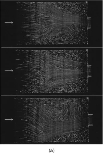
Figure 8. Influence of elasticity on the streakline flow patterns at the middle plane of a 4:1 square– square sudden contraction for PAA100 at Tⴝ 18.1ⴞ 0.2°C.
flow feature. However, the total Hencky strain is here un-changed because it is a function of the contraction ratio. Also of note here, the diverging streamlines with Boger fluids were observed in the absence of noticeable lip vortex activity. This contrasts with the visualizations of McKinley et al.8 in the
axisymmetric geometry, but agrees with their conclusions that diverging streamlines and lip vortex formation are probably unrelated.
As discussed more recently by Rothstein and McKinley,12
extensional viscosity alone does not explain the variety of flow features in contraction flows; hysteresis effects on the stress-conformation, normal stress effects in shear and extension, as well as contraction ratio and transient extensional viscosity behavior are relevant to the existence or not of a lip vortex and to the enhanced pressure drop, so the issue of diverging stream-lines should be at least as complex. In fact, the early experi-ments of Cable and Boger4-6had already shown strong
diverg-ing flow in the presence of combined shear-thinndiverg-ing and inertial effects, suggesting that inhomogeneous shear condi-tions near the wall are equally important. Quite interestingly, in the experiments of Walters and Rawlinson24in a 13.3:1
squar-e–square contraction, there is an abrupt expansion of the cen-tral jet as the fluid is just about to enter the smaller duct (cf. their Figure 5 at W⫽ 0.002), but there is already an enhanced vortex and the diverging streamlines may be related in part to the fluid particles being dragged into the recirculation, some-thing that we did not observe in our experiments.
The growth of the large vortex continues with elasticity, and the flow remains steady up to De2 ⬇ 52. At higher Deborah
numbers, the 3-D nature of the recirculating flow seems to have changed, as can be assessed by careful comparison of streak-lines in the recirculation at De2⫽ 50.4 with those taken at low
Deborah numbers. As the Deborah number further increases the flow becomes periodic, possibly because of an elastic instability, and this is observed by the crossings in some streaklines at De2 ⫽ 54.2. The amplitude of the oscillations
increases with De2, as seen in the three photos of Figure 9 taken
at three moments in time within a cycle for two different supercritical flow conditions. At even higher flow rates the flow loses its periodicity.
For the more concentrated Boger fluid, PAA300, the streak-line flow visualizations are shown in Figures 10a and 10b for conditions corresponding to two different temperatures, T ⫽ 21.0 and 17.5°C. The second set was taken 3 months after the first, with the same fluid sample (it was stored in a refrigerator), and with the purpose of checking the repeatability of the flow and absence of fluid degradation over time under the tested conditions. In general terms, the influence of Deborah number is the same as for PAA100, but a couple of important differ-ences are worth mentioning. First, the increase of the corner vortex located on the axial midplane at low Deborah numbers is also observed, but it is now more intense than that with the PAA100 fluid. This is clear in Figure 11, which compares the variation for both fluids of the vortex size in the midplane against the Deborah number (De2): for PAA300 xR/2H1peaks
by more than 25% relative to the Newtonian value at De2⬇ 6,
followed by a decrease to about 0.07 in the range De2⫽ 6 to
15. A second more important difference in relation to PAA100 is that a lip vortex is now clearly seen in the midplane for a certain range of Deborah numbers (see photos at De2⫽ 8.70
and 9.62 in Figure 10). In particular, at De2 ⫽ 9.62 when
inertia is still negligible, the lip vortex has similarities to that found for Boger fluids in the 4:1 plane contraction calculations of Alves et al.18(cf. their Figure 7 at De
2⫽ 4 for UCM fluids).
It is known from experimental and numerical work in the 4:1 plane sudden contraction flow with Boger fluids,23,44that a lip
vortex is formed at low to moderate Deborah numbers. This lip vortex grows with elasticity and eventually dominates the corner vortex, the characteristic flow feature of Newtonian flows and low-Deborah number viscoelastic flows. In contrast, for the axisymmetric sudden contraction flow of Boger fluids the corner vortex is normally found to grow with elasticity without the presence of any lip vortex35,45; there are exceptions
to this Boger fluid behavior, as in the experiments of Boger et al.9 and McKinley et al.8with PIB/PB solutions. Boger and
Binnington46also observed a lip vortex mechanism for a
PAA-based fluid in a 4:1 circular contraction with rounded corners, in deep contrast with the (usual) strong corner vortex enhance-ment observed in the same 4:1 circular contraction, but with a sharp reentrant corner. Rothstein and McKinley12argued about
the competing roles of extensional stresses and shear-induced normal stresses on vortex growth mechanisms, and concluded that lip vortices are associated with a domination of
shear-Figure 9. Streaklines for the flow of PAA100 in the mid-dle plane of a square–square contraction at three different moments within two different oscillating supercritical flow conditions.
induced elasticity, whereas corner vortex growth is dominated by extensional stresses, thus predominating at large contraction ratios and/or large Deborah numbers.
Given the similarities between the square–square contraction and the axisymmetric geometry in terms of both extensional strain rates developed along the centerline and the possibility of partial balance of cross-stream/azimuthal pressure and stress gradients, it comes as no surprise that the visualizations of Evans and Walters16for a square–square 16:1 contraction do
not show any lip vortex and instead illustrate a strong enhance-ment of the middle plane corner vortex (see their Figure 11). The presence of cross-stream secondary flows in the square contraction increases shear-induced normal stresses relative to those found in the corresponding circular contraction flow and, according to the above mechanism of Rothstein and McKinley, this will widen the range of contraction ratios where the lip
Figure 10. Influence of elasticity on the streakline flow patterns at the middle plane of a 4:1 square– square sudden contraction for PAA300.
vortex is observed. Such an effect is similar to rounding the reentrant corner in axisymmetric contractions: Rothstein and McKinley12report for this case the existence of a lip vortex for
the 4:1 contraction and a delay in corner vortex development, confirming the observations of Boger and Binnington.46
At higher flow rates/elasticity (De2 ⬎ 20) there is vortex
enhancement through a lip vortex mechanism. A diverging streakline pattern upstream of the contraction plane is also observed, but now in the presence of a lip vortex. The appear-ance of diverging streaklines in a 3-D square–square contrac-tion flow of Boger fluids, with and without lip vortex, is documented here for the first time and confirms the suggestion of McKinley et al.8 that the two phenomena are probably
unrelated. Simulations by Oliveira and Pinho42 for creeping
flow of UCM fluid in a 4:1 planar contraction corroborate this point, and the numerical results presented in Oliveira and Pinho43for the same flow under conditions where inertia is not
negligible (Re2 ⫽ 1) illustrate that inertial effects enhance
streamline divergence for high Deborah number flows. At even higher Deborah numbers, say for De2ⱖ 46.7 (De1
ⱖ 0.726), the flow of PAA300 becomes periodic, showing a behavior similar to that reported above for the PAA100 fluid. This periodic flow results from an elastic instability and occurs earlier than for the PAA100 solution, at De2⬵ 45 (De1⬵ 0.7).
Figure 12 shows three photos with the PAA300 solution per-taining to a cycle of events for two different supercritical flow
Figure 11. Variation of normalized vortex length with flow elasticity for Boger fluids PAA100 and PAA300.
Figure 12. Streaklines for the flow of PAA300 in the mid-dle plane of a square–square contraction at three different moments within oscillating su-percritical flow conditions.
(a) De2⫽ 55.1 and Re2⫽ 0.577; (b) De2⫽ 61.5 and Re2⫽
conditions, confirming that the average size of the time-dependent vortex continues to grow with Deborah number. Conclusions
Flow visualizations were carried out in the middle plane of a 4:1 square–square sudden contraction for Newtonian and Boger fluids under conditions of negligible inertia, using streakline photography. The Newtonian flow patterns were in good agreement with our own numerical results and show inertia to be negligible for Reynolds numbers below Re2⬇ 1.
The flow field was clearly three-dimensional, exhibiting open vortices with both Newtonian and viscoelastic fluids, and in-ertia tended to push the corner vortex toward the contraction plane.
For the two Boger fluids the upstream vortices were seen to increase slightly at low Deborah numbers, before an intense decrease took place leading to a minimum vortex size at De2⬇
15. As the Deborah number further increased, the streaklines on the central region of the approaching flow started to diverge, whereas the vortices grew strongly with elasticity until the flow became periodic and eventually chaotic at higher flow rates.
For the more concentrated Boger fluid (PAA300) these ef-fects were more intense because of the corresponding higher elasticity number, and a major difference in flow features was clearly seen: after the vortex attained its minimum size at intermediate Deborah numbers, 10ⱕ De2 ⱕ 15, a lip vortex
appeared and grew with elasticity. For the PAA100 solution, and although only corner vortex enhancement was observed, the variation of vortex size with Deborah number was compat-ible with the existence of a weak lip vortex (not captured with our visualization technique).
We speculate that the secondary flow in the cross section of the rectangular channel tends to increase the role of shear-induced normal stresses, thus leading to the appearance of a lip vortex at this contraction ratio and consequently delaying the vortex growth and instability to higher Deborah numbers, com-pared to the corresponding situation of a circular contraction. Such flow features, and the existence of a diverging flow well upstream of the contraction, are reported here for the first time in relation to the square–square contraction flow of Boger fluids. However, similar flow features have been previously reported for circular contractions.
Acknowledgments
The authors thank Prof. M. P. Gonc¸alves and D. Torres for help in characterizing the rheology of the fluids used in this work. M. A. Alves thanks Fundac¸a˜o Calouste Gulbenkian for financial support. Sponsorship of FEDER by the FCT program POCTI/EME/37711/2001 is gratefully acknowledged. Finally we are grateful for the relevant comments of one of the reviewers whose helpful suggestions significantly improved this article. Literature Cited
1. Van Dyke M. An Album of Fluid Motion. Stanford, CA: The Parabolic Press; 1982.
2. Boger DV, Walters K. Rheological Phenomena in Focus. Amsterdam: Elsevier; 1993.
3. Hassager O. Working group on numerical techniques. Fifth Interna-tional Workshop on Numerical Methods in Non-Newtonian Flows, Lake Arrowhead, USA. J Non-Newt Fluid Mech. 1988;29:2-5. 4. Cable PJ, Boger DV. A comprehensive experimental investigation of
tubular entry flow of viscoelastic fluids: Part I. Vortex characteristics in stable flow. AIChE J. 1978;24:868-879.
5. Cable PJ, Boger DV. A comprehensive experimental investigation of tubular entry flow of viscoelastic fluids: Part II. The velocity fields in stable flow. AIChE J. 1978;24:992-999.
6. Cable PJ, Boger DV. A comprehensive experimental investigation of tubular entry flow of viscoelastic fluids: Part III. Unstable flow. AIChE
J. 1979;25:152-159.
7. Nguyen H, Boger DV. The kinematics and stability of die entry flows.
J Non-Newt Fluid Mech. 1979;5:353-368.
8. McKinley GH, Raiford WP, Brown RA, Armstrong RC. Non linear dynamics of viscoelastic flow in axisymmetric abrupt contractions. J
Fluid Mech. 1991;223:411-456.
9. Boger DV, Hur DU, Binnington RJ. Further observations of elastic effects in tubular entry flows. J Non-Newt Fluid Mech. 1986;20:31-49. 10. Boger DV. Viscoelastic flows through contractions. Ann Rev Fluid
Mech. 1987;19:157-182.
11. Rothstein JP, McKinley GH. Extensional flow of a polystyrene Boger fluid through a 4:1:4 axisymmetric contraction/expansion. J Non-Newt
Fluid Mech. 1999;86:61-88.
12. Rothstein JP, McKinley GH. The axisymmetric contraction-expan-sion: The role of extensional rheology on vortex growth dynamics and the enhanced pressure drop. J Non-Newt Fluid Mech. 2001;98:33-63. 13. Phillips SD, Joo YL, Brown RA, Armstrong RC. Modeling and simulation of the flow through an axisymmetric contraction-expansion using a multi-mode Adaptive Length Scale model, Paper NF25, Proc of the XIV International Congress on Rheology (in CD-ROM), Seoul, Korea; 2004.
14. Ghosh I, Joo YL, McKinley GH, Brown RA, Armstrong RC. A new model for dilute polymer solutions in flows with strong extensional components. J Rheol. 2002;46:1057-1089.
15. Walters K, Webster MF. On dominating elastico-viscous response in some complex flows. Philos Trans R Soc Lond A Phys Sci. 1982;308: 199-218.
16. Evans RE, Walters K. Flow characteristics associated with abrupt changes in geometry in the case of highly elastic liquids. J Non-Newt
Fluid Mech. 1986;20:11-29.
17. Evans RE, Walters K. Further remarks on the lip-vortex mechanism of vortex enhancement in planar contraction flows. J Non-Newt Fluid
Mech. 1989;32:95-105.
18. Alves MA, Pinho FT, Oliveira PJ. Effect of a high-resolution differ-encing scheme on finite-volume predictions of viscoelastic flows. J
Non-Newt Fluid Mech. 2000;93:287-314.
19. Alves MA, Oliveira PJ, Pinho FT. Benchmark solutions for the flow of Oldroyd-B and PTT fluids in planar contractions. J Non-Newt Fluid
Mech. 2003;110:45-75.
20. White SA, Baird DG. The importance of extensional flow properties on planar entry flow patterns of polymer melts. J Non-Newt Fluid
Mech. 1986;20:93-101.
21. White SA, Baird DG. Flow visualization and birefringence studies on planar entry flow behaviour of polymer melts. J Non-Newt Fluid Mech. 1988;29:245-267.
22. White SA, Baird DG. Numerical simulation studies of the planar entry flow of polymer melts. J Non-Newt Fluid Mech. 1988;30:47-71. 23. Nigen S, Walters K. Viscoelastic contraction flows: Comparison of
axisymmetric and planar configurations. J Non-Newt Fluid Mech. 2002;102:343-359.
24. Walters K, Rawlinson DM. On some contraction flows for Boger fluids. Rheol Acta. 1982;21:547-552.
25. Xue SC, Phan-Thien N, Tanner RI. Numerical investigations of La-grangian unsteady extensional flows of viscoelastic fluids in 3-D rectangular ducts with sudden contractions. Rheol Acta. 1998;37:158-169.
26. Mompean G, Deville M. Unsteady finite volume simulation of Old-royd-B fluid through a three-dimensional planar contraction. J
Non-Newt Fluid Mech. 1997;72:253-279.
27. Xue SC, Phan-Thien N, Tanner RI. Three dimensional numerical simulations of viscoelastic flows through planar contractions. J
Non-Newt Fluid Mech. 1998;74:195-245.
28. Stokes JR. Swirling Flow of Viscoelastic Fluids. PhD Dissertation. Melbourne, Australia: Dept. of Chemical Engineering, University of Melbourne; 1998.
29. Barnes HA. A Handbook of Elementary Rheology. Aberystwyth, Wales: Institute of Non-Newtonian Fluid Mechanics, University of Wales; 2000.
Theoret-ical and Experimental Analysis (in Portuguese). PhD Dissertation.
Porto, Portugal: Dept. of Chemical Engineering, University of Porto; 2004.
31. Bird RB, Armstrong RC, Hassager O. Dynamics of Polymeric Liquids.
Volume 1: Fluid Dynamics. New York, NY: Wiley; 1987.
32. Quinzani LM, McKinley GH, Brown RA, Armstrong RC. Modeling the rheology of polyisobutylene solutions. J Rheol. 1990;34:705-748. 33. Phan-Thien N. Cone-and-plate flow of the Oldroyd-B fluid is unstable.
J Non-Newt Fluid Mech. 1985;17:37-44.
34. McKinley GH, Byars JA, Brown RA, Armstrong RC. Observations on the elastic instability in cone-and-plate and parallel-plate flows of a polyisobutylene Boger fluid. J Non-Newt Fluid Mech. 1991;40:201-229.
35. Alves MA, Oliveira PJ, Pinho FT. Numerical simulation of viscoelas-tic contraction flows. In: Bathe KJ, ed. Computational Fluid and Solid
Mechanics. Amsterdam: Elsevier; 2003:826-829.
36. Alves MA, Oliveira PJ, Pinho FT. A convergent and universally bounded interpolation scheme for the treatment of advection. Int J
Numer Methods Fluids. 2003;41:47-75.
37. Chiang TP, Sheu TWH, Wang SK. Side wall effects on the structure of laminar flow over a plane-symmetric sudden expansion. Comput
Fluids. 2000;29:467-492.
38. Schreck E, Scha¨fer M. Numerical study of bifurcation in three-dimen-sional sudden channel expansions. Comput Fluids. 2000;29:583-593. 39. Williams PT, Baker AJ. Numerical simulations of laminar flow over a 3D backward-facing step. Int J Numer Methods Fluids. 1997;24:1159-1183.
40. Biswas G, Breuer M, Durst F. Backward-facing step flows for various expansion ratios at low and moderate Reynolds numbers. ASME J
Fluids Eng. 2004;126:362-374.
41. Alves MA, Oliveira PJ, Pinho FT. On the effect of contraction ratio in viscoelastic flow through abrupt contractions. J Non-Newt Fluid Mech. 2004;122:117-130.
42. Oliveira PJ, Pinho FT. Plane contraction flows of Upper Convected Maxwell and Phan-Thien–Tanner fluids as predicted by a finite-vol-ume method. J Non-Newt Fluid Mech. 1999;88:63-88.
43. Oliveira PJ, Pinho FT. Numerical procedure for the computation of fluid flow with arbitrary stress–strain relationships. Num Heat Transfer
B. 1999;35:295-315.
44. Walters K, Webster MF. The distinctive CFD challenges of computa-tional rheology. Int J Numer Methods Fluids. 2003;43:577-596. 45. Sasmal GPA. Finite-volume approach for calculation of viscoelastic
flow through an abrupt axisymmetrical contraction. J Non-Newt Fluid
Mech. 1995;56:15-47.
46. Boger DV, Binnington RJ. Experimental removal of the re-entrant corner singularity in tubular entry flows. J Rheol. 1994;38:333-349. 47. Purnode B, Crochet MJ. Flows of polymer solutions through
contrac-tions. Part 1: Flows of polyacrylamide solutions through planar con-tractions. J Non-Newt Fluid Mech. 1996;65:269-289.
48. Quinzani LM, Armstrong RC, Brown RA. Birefringence and laser-Doppler velocimetry (LDV) studies of viscoelastic flow through a planar contraction. J Non-Newt Fluid Mech. 1994;52:1-36.