Color vision models : some simulations, a general n-dimensional model, and the colourvision R package

Ecology and Evolution. 2018;8:8159–8170. www.ecolevol.org  

|

1 | INTRODUCTION

The study of proximate and ultimate causes of animal coloration has played a significant role in our understanding of evolutionary

processes (for a review on the study of coloration see Cuthill et al., 2017). To study the selective forces acting on an organism coloration, it is crucial to understand how color patches are perceived by po-tential selective agents (e.g. a predator; Endler, 1990). Furthermore,

Received: 19 January 2018 

|

|

O R I G I N A L R E S E A R C H

Color vision models: Some simulations, a general n- dimensional

model, and the colourvision R package

Felipe M. Gawryszewski

This is an open access article under the terms of the Creative Commons Attribution License, which permits use, distribution and reproduction in any medium, provided the original work is properly cited.

© 2018 The Authors. Ecology and Evolution published by John Wiley & Sons Ltd. Departamento de Zoologia, Instituto de

Ciências Biológicas, Universidade de Brasília, Brasília, Brazil

Correspondence

Departamento de Zoologia, Instituto de Ciências Biológicas, Universidade de Brasília, Brasília, Brazil.

Email: f.gawry@gmail.com

Abstract

The development of color vision models has allowed the appraisal of color vision in-dependent of the human experience. These models are now widely used in ecology and evolution studies. However, in common scenarios of color measurement, color vision models may generate spurious results. Here I present a guide to color vision modeling (Chittka (1992, Journal of Comparative Physiology A, 170, 545) color hexa-gon, Endler & Mielke (2005, Journal Of The Linnean Society, 86, 405) model, and the linear and log- linear receptor noise limited models (Vorobyev & Osorio 1998,

Proceedings of the Royal Society B, 265, 351; Vorobyev et al. 1998, Journal of Comparative Physiology A, 183, 621)) using a series of simulations, present a unified

framework that extends and generalize current models, and provide an R package to facilitate the use of color vision models. When the specific requirements of each model are met, between- model results are qualitatively and quantitatively similar. However, under many common scenarios of color measurements, models may gener-ate spurious values. For instance, models that log- transform data and use relative photoreceptor outputs are prone to generate spurious outputs when the stimulus photon catch is smaller than the background photon catch; and models may generate unrealistic predictions when the background is chromatic (e.g. leaf reflectance) and the stimulus is an achromatic low reflectance spectrum. Nonetheless, despite differ-ences, all three models are founded on a similar set of assumptions. Based on that, I provide a new formulation that accommodates and extends models to any number of photoreceptor types, offers flexibility to build user- defined models, and allows users to easily adjust chromaticity diagram sizes to account for changes when using differ-ent number of photoreceptors.

K E Y W O R D S

chromaticity diagram, color hexagon, color space, color triangle, color vision model, receptor noise-limited model

animal vision may also evolve in response to environmental condi-tions, as is suggested by the correlation between light conditions and peak wavelength sensitivities of marine mammal photoreceptors (Fasick & Robinson, 2000).

There are several axes of variation in animal vision, such as density and distribution of receptors in the retina (Hart, 2001), eye resolution (Land & Nilsson, 2012), and presence of oil- droplets in photoreceptors cells (Hart, Partridge, Bennett, & Cuthill, 2000). In terms of color vision, the most obvious differences are found in the spectral sensitivity of photoreceptors cells (Kelber, Vorobyev, & Osorio, 2003; Osorio & Vorobyev, 2008). For instance, most non-mammal vertebrates are tetrachromats, most insects are trichro-mats, and, contrary to mammals, both have a color perception that spans into the ultraviolet (Bowmaker, 1998; Briscoe & Chittka, 2001; Kelber et al., 2003; Osorio & Vorobyev, 2008). A fascinating illus-tration of how photoreceptor sensitivity may affect perceptual dif-ferences comes from human subjects that have undergone cataract treatment. The sensitivity curve of the human blue photoreceptor spans into the ultraviolet (UV) range, but humans are UV- insensitive because pigments in crystallin filter out wavelengths below 400 nm. Cataract surgery occasionally replaces the crystallin with a UV- transmitting lens, and anecdotal evidence suggests that those in-dividuals are then able to see the world differently: new patterns are observed in flower petals, some garments originally perceived as black appear purple, and black light is perceived as blue light (Cornell, 2011; Stark & Tan, 1982).

Thus, studies of animal coloration can clearly benefit from ap-praisals of how color patches are perceived by nonhuman observ-ers. Moreover, the same color patch may be perceived differently depending not only on the observer, but also on the conditions of exposure of the color patch (e.g. background color and environmen-tal light conditions; Endler, 1990). With the advent of affordable spectrometers for reflectance measurements, application of color vision models became commonplace in the ecology and evolution subfields (Kemp et al., 2015). Together, some of the most important color vision papers have been cited over 2,800 times (Endler, 1990 (919); Vorobyev & Osorio, 1998 (601), Vorobyev, Osorio, Bennett, Marshall, & Cuthill, 1998 (460); Chittka, 1992 (324); Chittka, Beier, Hertel, Steinmann, & Menzel, 1992 (128); Endler & Mielke, 2005 (445); Google Scholar search on October 31st 2016).

Knowledge of model strength and limitations is crucial to as-sure reproducible and meaningful results from model applications. Thus, the motivation of this study is twofold: firstly, to compare and illustrate the consistency of between- model results in com-mon scenarios of color measurements; and secondly, to facilitate the use of color vision models by evolutionary biologists and ecolo-gists by giving a unified framework which extends and generalizes the most commonly used color vision models. I did not aim to give an in- depth analysis of the physiology of color vision, but rather, to provide a practical guide to the use of color vision models and to demonstrate their limitations and strengths so that users avoid the common pitfalls of color vision modeling. Guidance on other aspects of color vision models can be found elsewhere (Bitton,

Janisse, & Doucet, 2017; Endler & Mielke, 2005; Hempel de Ibarra, Vorobyev, & Menzel, 2014; Kelber et al., 2003; Kemp et al., 2015; Lind & Kelber, 2009; Olsson, Lind, & Kelber, 2017a,b; Osorio & Vorobyev, 2008; Renoult, Kelber, & Schaefer, 2017; Vorobyev, Osorio, Peitsch, Laughlin, & Menzel, 2001; White, Dalrymple, Noble, & O’Hanlon, 2015).

2 | GUIDELINES AND LIMITATIONS

As any model, color vision models are simplified representations of reality. Their mathematical formulation imposes limits to their pre-dictive power. Many of these limitations have been pointed out by several authors (Bitton et al., 2017; Lind & Kelber, 2009; Vorobyev, 1999; Vorobyev & Brandt, 1997; Vorobyev, Hempel de Ibarra, Brandt, & Giurfa, 1999). Nonetheless, as stressed recently, several papers in the evolution and ecology subfields still misuse color vision models (Marshall, 2017; Olsson et al., 2017b). Some of these limita-tions may be obvious to scientists working directly on color vision, but are not by many nonspecialists that apply color vision models to their research. In this section, I compile and illustrate those limita-tions by a series of simulations. My focus is on the limitations arising from the mathematical formulation of each model, which are often obscure to many nonspecialists in the field.

I modeled the perception of the honeybee (Apis mellifera) using the following color vision models: Chittka (1992) color hexagon model (hereafter CH model), Endler and Mielke (2005) model (here-after EM model), and linear and log- linear versions of the receptor noise model (hereafter linear- RNL and log- RNL models (Vorobyev et al., 1998; Vorobyev & Osorio, 1998). I began with a basic model setup using simulated data. I then proceeded to make a series of changes to this basic model to illustrate how models behave with typical input data used in ecology and evolution papers. At the end, I used real flower reflectance data to compare model results. I vio-lated some model assumptions, for example, I applied the linear- RNL model to nonsimilar colors, so that model behaviour could be visual-ized under suboptimum conditions.

Human color perception can be divided into two components: the chromatic (hue and saturation) and achromatic (brightness/ intensity) dimensions. These models are representations of the chromatic component of color vision (Renoult et al., 2017). Color vision models are based on photoreceptor photon catches of each photoreceptor type in the retina. Photon catches depend on the illuminant spectrum reaching the observed object, the reflec-tance of the observed object, the sensitivity curve of photorecep-tors, and the background reflectance (for details see Supporting Information Appendix S1).

These models assume that color vision is achieved by neural op-ponency mechanisms, which is supported by experimental data (Kelber et al., 2003; Kemp et al., 2015, but see Thoen, How, Chiou, & Marshall, 2014 for an exception to this rule). The exact opponent channels are usually not known (Kelber et al., 2003; Kemp et al., 2015), but empir-ical studies suggest that the exact opponency channels do not need

to be known for a good prediction of behavioural responses by color vision models (Cazetta, Schaefer, & Galetti, 2009; Chittka et al., 1992; Spaethe, Tautz, & Chittka, 2001; Vorobyev & Osorio, 1998). Taking that into account, the three models presented here assume that inputs from photoreceptors are weighted equally and are all opposed against each other.

In addition, photoreceptor values are adjusted taking into consid-eration the photon catch arising from the environment background (Supporting Information Appendix S1, Equation S3), which tries to emulate the physiological adaptation of photoreceptors to the envi-ronmental light conditions and the color constancy (Chittka, Faruq, Skorupski, & Werner, 2014). Photon catches relative to the background are then transformed to represent the relationship between photore-ceptor input and output. Each model will apply a different transforma-tion (e.g. identity, ln, hyperbolic; for details see Supporting Informatransforma-tion Appendix S1), but the rationale behind all these are the nonlinear rela-tionship between photoreceptor input and output. However, only the EM (Endler & Mielke, 2005) and log- RNL models (Vorobyev et al., 1998) apply the natural logarithm as formulated by the Fechner- Weber law of psychophysics. The CH model applies a hyperbolic transformation that also simulates a nonlinear relationship between photoreceptor input and output, and the linear RNL models is to be applied only to simi-lar colors so that the relationship is nearly linear (Vorobyev & Osorio, 1998). Furthermore, EM model uses only relative photoreceptor out-put values (sum of photoreceptor values equal 1), not their absolute values, which is based on the biological observation that only relative differences in photoreceptor outputs are used in a color opponency mechanisms (Endler & Mielke, 2005).

2.1 | First simulation: basic setup

I used honeybee worker (A. mellifera) photoreceptor sensitivity curves (data from Peitsch et al., 1992 available in Chittka & Kevan, 2005; Supporting Information Figure S1a). For the background re-flectance spectrum, I created a theoretical achromatic rere-flectance with a constant 7% reflectance across 300–700 nm (Supporting Information Figure S1b). For the illuminant, I used the CIE D65, a reference illuminant that corresponds to midday open- air condi- tions (Supporting Information Figure S1c). In addition, RNL mod-els assume that, under bright light conditions, color discrimination threshold is limited by photoreceptor noise (Vorobyev & Osorio, 1998; for dim light conditions shot noise also limits discrimina-tion; Vorobyev et al., 1998; see Olsson et al., 2017a for a recent review). For these models, I used measurements of honeybee photoreceptor noise (0.13, 0.06 and 0.12 for short- , medium- , and long- wavelength photoreceptors; data from Peitsch, 1992 avail-able in Vorobyev & Brandt, 1997). With respect to the stimulus reflectance spectra, I generated reflectance curves using a logis-tic function (see Supporting Information Appendix S1 for details). I generated curves with reflectance values from of 10% to 60%, and midpoints varying from 300 to 700 nm with 5 nm intervals, in a total of 81 reflectance spectra (Supporting Information Figure S1d). For each model, I calculated photoreceptor outputs, color

loci (x and y), and the chromatic distance to the background (ΔS) for each reflectance spectra using equations for CH, EM, and RNL models (Equations S2–S19 see Supporting Information Appendix S1 for details on model calculations). To illustrate the generality of the results from these simulations, I ran the same simulations with a Gaussian function to generate the stimulus reflectance spectra, and for tetrachromatic avian vision (see Supporting Information Appendix S1 for methods and results; results are qualitatively very similar to the original simulations).

In this first setup, models are congruent with respect to their results. The chromaticity diagrams indicate a similar relative position of reflectance spectra between models (Figure 1). All of them esti-mate a bell- shaped ΔS curve, with maximum values around a 500- nm midpoint wavelength (Figure 1).

2.2 | Second simulation: stimulus reflectance lower

than background reflectance

In the second simulation, I removed 10 percentage points to the stimulus reflectance spectra (Supporting Information Figure S2a). In this case, my aim was to (a) analyze how a relatively small change in reflectance curves affect model results, as small changes in overall reflectance values may be an artifact of spectrometric measurement error (for guidance on spectrometric reflectance measurements, see Anderson & Prager, 2006); and (b) to create reflectance spectra that would generate a lower photoreceptor response from stimulus than the background.

In this simulation, results projected into chromaticity diagrams show differences between model predictions of color perception for the same reflectance spectrum (Figure 2). Contrary to the first simu-lation, in the EM model, points follow two lines increasing in opposite directions, with data points reaching values outside color space limits (Figure 2b). The EM model estimates spurious ΔS values for reflec-tance curves with midpoints between 450 and 550 nm (Figure 2b). A maximum ΔS of 116 is reached at 490 nm midpoint wavelength; how-ever, by the model definition, the ΔS maximum value is 0.75 (Endler & Mielke, 2005). Photoreceptor outputs also reach nonsensical negative values and values above 1 (by model definition, maximum photorecep-tor output should vary between 0.0 and 1.0; Figure 2b). This happens when relative photon catches (q_i; Equation S4, Supporting Information Appendix S1) are below 1 (i.e. background photon catch is higher than stimulus photon catch), and therefore, the ln- transformation gener-ates negative values. Consequently, the denominator in Supporting Information Equation S9 may reach values close to zero, which causes photoreceptor outputs to tend to infinity.

Comparable to the EM model, the log- RNL model generates nonsensical negative photoreceptor excitation values (Figure 2d). Again, this happens because when the relative photoreceptor pho-ton catch (q_i; Equation S4, Supporting Information Appendix S1) is below 1, the ln- transformation generates negative values (Equation S15, Supporting Information Appendix S1). Consequently, this model now presents a sigmoid ΔS, increasing from short to long midpoint wavelengths (maximum ΔS at 700 nm; Figure 2d).

Therefore, color vision models, especially those that are log- transformed (EM model and log- RNL model) and convert photore-ceptor output to relative values (EM model), are prone to produce nonsensical results when the observed reflectance generates a lower response than the background (Q_i < Q_Bi; Equation S4, Supporting Information Appendix S1).

The transformation of photoreceptor inputs also illustrates a common misconception related to the use of color vision models. Models are intended to be insensitive to variation in intensity only. Nonetheless, in practice, models are insensitive to variation in photo-receptor outputs as long as the difference between outputs remains the same. However, this does not mean that reflectance spectra that only differ in intensity will generate identical model outputs. For in-stance, a reflectance spectrum that generates photoreceptor out-puts of E₁ = 0.1, E₂ = 0.2 and E₃ = 0.3 will lie at the exact same color locus coordinates as another reflectance that generates photorecep-tor outputs of E₁ = 0.2, E₂ = 0.3, and E₃ = 0.4 because differences

between photoreceptor outputs remain the same (i.e. E₃ − E₁ = 0.2;

E₂ − E₁ = 0.1; and E₃ − E₂ = 0.1). Nonetheless, reflectance spectra that differ only in intensity (simulation 1 vs. simulation 2) will most likely generate distinct differences between photoreceptor outputs because of the photoreceptor transformation. Consequently, these spectra will lie at different positions in the animal color space (color locus coordinates; compare Figures 1 and 2). CH model, in special, predicts different color loci for reflectance curves that only differ in intensity due to the hyperbolic transformation (Chittka, 1992). There is a controversy whether this represents a biological phenomenon (Chittka, 1992, 1999) or it is a model limitation (Vorobyev et al., 1999).

2.3 | Third simulation: achromatic stimulus and

chromatic background

In the basic model, I used an achromatic reflectance spectrum (7% reflectance from 300 to 700 nm). In practice, however, most

F I G U R E   1   Chromaticity diagrams, ΔS, and photoreceptor outputs of the basic setup of color vision model simulations: (a) Chittka (1992)

color hexagon (CH), (b) Endler and Mielke (2005) color triangle (EM), and (c) linear and (d) log- linear Receptor Noise Limited models (Linear- RNL and Log- RNL; Vorobyev & Osorio, 1998; Vorobyev et al., 1998). Colors in chromaticity diagrams correspond to reflectance spectra from Supporting Information Figure S1d. ΔS- values (middle row) and photoreceptor outputs (bottom row) as a function of reflectance spectra with midpoints from 300 to 700 nm. Violet, blue, and green colors represent short, middle, and long λmax photoreceptor types, respectively.

Vertical lines represent the midpoint of maximum ΔS- values

E2 E1 E3 CH u s m EM –40 0 40 –40 04 0 E1 E2 E3 x y Linear-RNL –10 0 10 –10 0 10 E1 E2 E3 x y Log-RNL 0. 0 0. 5 1. 0 S 0. 00 .5 1. 0 02 04 0 0 5 10 300 500 700 0. 0 0. 51 .0 Midpoint (nm) Photoreceptor output –1 01 05 10 0. 01 .5 3. 0 (a) (b) (c) (d)

studies that apply color vision models use chromatic reflectance backgrounds, such as a leaf (e.g. Vorobyev et al., 1998), or an aver-age of background- material reflectance spectra (e.g. Gawryszewski & Motta, 2012). Models are constructed so that the background re-flectance spectrum lies at the center of the color space. Vorobyev and Osorio (1998) specifically state that their linear receptor noise model is designed to predict perception of large targets, in bright light conditions and against an achromatic background. Despite this, given that photoreceptors adapt to the light environment condition, usage of chromatic background is probably reasonable (Vorobyev et al., 1998). I generated achromatic reflectance spectra ranging from 5% to 95% in 10 percent point intervals (Supporting Information Figure S2b), and instead of having an achromatic background, I used a chromatic background (Supporting Information Figurre S2c). The background is the average reflectance of leaves, leaf litter, tree bark, and twigs collected in an area of savanna vegetation in Brazil (data from Gawryszewski & Motta, 2012).

The chromatic background causes differences in background photoreceptor photon catches. Consequently, achromatic reflec-tance spectra do not lie at the center of the color spaces as would be expected. The CH model shows a maximum ΔS value of 0.31 at 5% reflectance achromatic spectrum (Figure 3a). ΔS values then decrease as the reflectance value of achromatic spectra increases (Figure 3a). The EM model produces spurious values at 5% reflec-tance achromatic spectrum because it generates negative photore-ceptor output values (Figure 3b). From 15% and beyond, ΔS values then decrease as the reflectance value of achromatic spectra in-creases (Figure 3b). The linear- RNL model shows a linear increase in ΔS values as the reflectance value of achromatic spectra increases (Figure 3c). Similarly, photoreceptor outputs also increase linearly as the reflectance value of achromatic spectra increases, but with different slopes for each photoreceptor type (Figure 3c). Contrary to other models, ΔS- values in the log- RNL model do not change with varying reflectance values of achromatic spectra (Figure 3d).

F I G U R E   2   Chromaticity diagrams, ΔS, and photoreceptor outputs of the second simulation—10 percentage points removed from

reflectance values: (a) Chittka (1992) color hexagon (CH), (b) Endler and Mielke (2005) color triangle (EM), and (c) linear and (d) log- linear Receptor Noise Limited models (Linear- RNL and Log- RNL; Vorobyev & Osorio, 1998; Vorobyev et al., 1998). Colors in chromaticity diagrams correspond to reflectance spectra from Supporting Information Figure S2d. ΔS- values (middle row) and photoreceptor outputs (bottom row) as a function of reflectance spectra with midpoints from 300 to 700 nm. Violet, blue, and green colors represent short, middle, and long λmax

photoreceptor types, respectively. Vertical lines represent the midpoint of maximum ΔS-values

E2 E1 E3 CH u s m EM –40 0 40 –40 04 0 E1 E2 E3 x y Linear-RNL –40 0 40 –40 0 40 E1 E2 E3 x y Log-RNL 0. 0 0. 5 1. 0 S 0. 00 .5 1. 0 02 04 0 02 04 0 300 500 700 0. 0 0. 51 .0 Midpoint (nm) Photoreceptor output –1 01 05 10 –10 –5 05 (a) (b) (c) (d)

Although photoreceptor outputs increase as reflectance value of achromatic spectra increases (Figure 3d), the difference between photoreceptor outputs remains the same. Consequently, ΔS- values do not change.

This simulation shows that CH and EM models predict coun-terintuitive values because a highly reflective achromatic stimulus is predicted to have a lower ΔS- value than a spectrum with simi-lar reflectance to the background. This phenomenon has already been discussed previously both theoretically and experimentally (Stoddard & Prum, 2008; Vorobyev, 1999; Vorobyev & Brandt, 1997; Vorobyev et al., 1999). For instance, in a laboratory experi-mental setup, Vorobyev et al. (1999) showed that bees made more mistakes when trying to detect a grey target against a green back-ground than when trying to detect a white target again the same green background.

Another common misconception arises from the use of detect-ability/discriminability thresholds. The RNL model, for instance, is a good predictor of the detectability of monochromatic light against a gray background (Vorobyev & Osorio, 1998). For this model, and given the experimental condition, a ΔS = 1 equals one unit of just noticeable difference (JND; Vorobyev & Osorio, 1998). However, this threshold is not fixed. For zebra finches, for instance, the same pair of similar red objects have a discriminability threshold of ca. 1 JND when the background is red, but much higher when the back-ground is green (Lind, 2016). Furthermore, the relationship between ΔS values and probability of discriminability varies between species and it is not necessarily linear, in particular for ΔS values that greatly surpass threshold values (Garcia, Spaethe, & Dyer, 2017). In addition,

correct model parametrization is vital for RNL models, which are very sensitive to correct photoreceptor noise values (Lind & Kelber, 2009; Olsson et al., 2017a) and the relative abundance of photore-ceptors in the retina (Bitton et al., 2017).

2.4 | Real reflectance data: comparison

between models

In this setup, my aim was to compare model results using real reflec-tance data. I used 858 reflecreflec-tance spectra from flower parts col-lected worldwide and deposited in the Flower Reflectance Database (FReD; Arnold, Faruq, Savolainen, McOwan, & Chittka, 2010). I used only spectrum data that had a wavelength range from 300 to 700 nm. Data were then interpolated to 1- nm intervals and negative values converted to zero. I used the same reflectance background from simulation 03, and other model parameters identical to the basic model setup. I compared model results visually, and by test-ing the pairwise correlation between the model’s ΔS values. I used the Spearman correlation coefficient because data did not fulfill as-sumptions for a parametric test.

When real flower reflectance spectra are used, models also give different relative perception for the same reflectance spec- trum. The results of the CH model and the log- RNL model are sim-ilar both qualitatively and quantitatively: color loci projected into the color space (Supporting Information Figure S3) show a similar relative position of reflectance spectra, and there is a high cor-relation score between ΔS values (ρ = 0.884; N = 858; p < 0.001). Even though many EM points lie outside the chromaticity diagram

F I G U R E   3   Third setup of color vision model simulations—achromatic stimulus against chromatic background: (a) Chittka (1992) color

hexagon (CH), (b) Endler and Mielke (2005) color triangle (EM), and (c) linear and (d) log- linear Receptor Noise Limited models (Linear- RNL and Log- RNL; Vorobyev & Osorio, 1998; Vorobyev et al., 1998). ΔS- values (top row) and photoreceptor outputs (bottom row) as a function of spectra with achromatic reflectance from 5% to 95%. Violet, blue, and green colors represent short, middle, and long λmax photoreceptor

types, respectively 0. 0 0. 51 .0 S CH 0. 0 0. 51 .0 _EM 0 110 220 Linear-RNL 0 10 20 _Log-RNL 0 50 100 0. 00 .5 1. 0 Achromatic reflectance (%) Photoreceptor output –1 01 02 55 0 –5 0 5 (b) (a) (c) (d)

(Supporting Information Figure S3b), results suggest a high concor-dance between CH and EM models (ρ = 0.889; N = 858; p < 0.001). There was moderate concordance between the linear and log versions of the RNL model (ρ = 0.434; N = 858; p < 0.001) and be-tween the EM and log- RNL models (ρ = 0.662; N = 858; p < 0.001). Finally, there was poor concordance between the linear- RNL model and both EM models (ρ = −0.264; N = 858; p < 0.001), as well as the linear-RNL and CH models (ρ = 0.037; N = 858; p = 0.278).

In addition to the limitations commented above, these models also do not incorporate higher order cognition abilities that may af-fect how color is perceived (Dyer, 2012). In bees, for instance, pre-vious experience, learning and experimental conditions may affect their behavioural discriminability thresholds (Chittka, Dyer, Bock, & Dornhaus, 2003; Dyer, 2012; Dyer & Chittka, 2004; Dyer, Paulk, & Reser, 2011; Giurfa, 2004), and in humans, the ability to discriminate between colors is affected by the existence of linguistic differences for colors (Winawer et al., 2007). Moreover, models presented here are pairwise comparisons between color patches, which do not in-corporate the complexity of an animal color pattern composed of a mosaic of color patches of variable sizes. Endler and Mielke (2005) provide a methodological and statistical tool that can deal with a cloud of points representing an organism’s color patches. Use of hyperspec-tral cameras or adapted DSLR cameras may facilitate the analysis of animal coloration as a whole (Chiao, Wickiser, Allen, Genter, & Hanlon, 2011; Stevens, Párraga, Cuthill, Partridge, & Troscianko, 2007). Other aspects that may be important when detecting a target, such as size, movement, light polarization (Cronin, Johnsen, Marshall, & Warrant, 2014), and color categorization (Hempel de Ibarra et al., 2014; Kelber & Osorio, 2010), are also not incorporated into those models.

Therefore, accurate application of color vision models depends on the inspection of photoreceptor output values, knowledge of model assumptions, comprehension of the mathematical formula used for constructing each model, and familiarity with mechanisms of color vision of the animal being modeled. Comparison of model results with field and laboratory- based behavioural experiments are also crucial to complement and validate model results.

3 | A GENERIC METHOD FOR N-

DIMENSIONAL MODELS

Despite some differences between these models, they can all be understood using the same general formulae. As explained in the section above, color vision is achieved by neural opponency mechanisms (Kelber et al., 2003; Kemp et al., 2015), although for most species the opponency channels have not been identified (Kelber et al., 2003; Kemp et al., 2015). In practice, the solution is to build a model so that all photoreceptor outputs are compared simultaneously. This is achieved by projecting photoreceptor out-puts as vectors (vector lengths represent output values) into a space so that all vectors have the same pairwise angle (i.e. the resulting vector has length zero when all vector lengths are equal; Figure 4). Each model will present differently arranged vectors.

However, they can all be reduced to the same general formula because vector position in relation to the axes has no biological significance as long as they preserve the same pairwise angle (see Vorobyev & Osorio, 1998).

By adding vectors, the length of the resultant vector represents the chromaticity distance of the stimulus against the background, and vector components represent the stimulus coordinates in the color space (color locus; Chittka, 1992). Vorobyev and Osorio (1998) assume that noise at photoreceptors limits chromatic dis-crimination. In this case, each photoreceptor has a specific noise, and the chromaticity distance is given by the resultant photore-ceptor length divided by its noise (see calculation below; Figure 4). For a generic n- dimensional method, let i be the number of photoreceptor sensitivity curves. Assuming an opponency mech-anism, the animal chromaticity diagram will have n = i − 1 dimen-sions. In this space, there will be i vectors, each representing the output of one photoreceptor type (Figure 4a). Each vector will have i − 1 components (n = i − 1), each representing one coordi-nate in the chromaticity diagram (Figure 4a). Photoreceptors are assumed to be weighted equally and give sum zero; therefore, their pairwise angle is given by:

Then, the last component of a generic unit vector (v = [v₁, v₂, v₃ …

vn]) projected into a chromaticity diagram with n = i − 1 dimensions

can be found by the following equations:

If the chromaticity diagram has only one dimension, (i = 2), then the generic vector has only one component (n = 1), given by Equation 2. For a chromaticity diagram with more than one dimen-sion (i > 2), other vector components are found by the following equation:

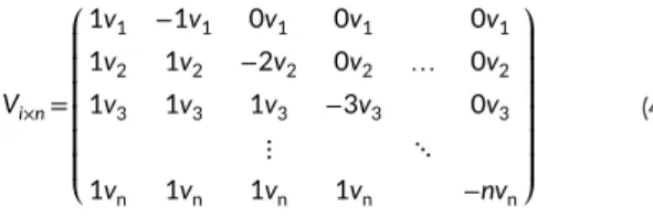
where n is the total number of vector components, and k = (1, 2, 3, …, n − 1). Then a matrix of column vectors (size: i × n; each column represents one vector) with unit vectors equidistant from each other can be found by the following equation:

where v is the generic unit vector, as found by Equations 1–3. Equations 1–4 were found empirically. (1) 𝜃 =arccos ( −1 n ) . (2) v[n]=cos(𝜃). (3) v[n−k]= − 1 n − k √ √ √ √1− ∑n m = n−k+1 v2 m (4) V_i×n= ⎛ ⎜ ⎜ ⎜ ⎜ ⎜ ⎜ ⎝ 1v₁ −1v₁ 0v₁ 0v₁ 0v₁ 1v₂ 1v₂ −2v₂ 0v₂ … 0v₂ 1v3 1v3 1v3 −3v3 0v3 ⋮ ⋱ 1v_n 1v_n 1v_n 1v_n −nvn ⎞ ⎟ ⎟ ⎟ ⎟ ⎟ ⎟ ⎠

Note that this is one of infinite possible solutions to project n vectors into a (n − 1) dimensional space. Although it will not have a biological meaning, nor affect results, other orientations of matrix V can be achieved by vector rotation matrices.

With matrix V, one can find a vector, whose components rep-resent coordinates in the color space (X₁, X₂, …, X_n), by multiplying matrix V by a column vector with photoreceptor output as its com-ponents (p = (p₁, p₂, p₃, … p_i)):

One may also represent Equation 6 as formulae, as is usually per-formed when presenting color vision models.

Matrix V can be manipulated to accommodate different color vi-sion models. Chittka (1992) assumes a maximum vector length of one (Equation S5, Supporting Information Appendix S1); therefore, matrix V can be used directly. The tetrachromatic version of Endler and Mielke (2005), however, assumes a maximum length of 0.75. Therefore, matrix V must be multiplied by a scalar with the desired length (see Supporting Information Appendix S1 for detail on model calculation using formulae above).

In the original study, Vorobyev and Osorio (1998) provided a method to calculate chromaticity distances (ΔS) independently of the matrix V, and their method is already applicable to any number

of photoreceptor types (see also Clark et al. 2017 to another model extension). However, within Vorobyev and Osorio (1998) formulation, it is possible to find a space representing RNL model color space in terms units of receptor noise (see for instance Renoult et al., 2017 and Pike, 2012a,b). For a 2- D color space, the noise standard deviation will be given by the line segment, from the centre to the edge of the standard deviation contours, in the same direction as the vector representing the signal (Figure 4b). Then a vector, (⃗_{s), whose components represent coordinates in}

the color space, is found by dividing vector components by the length of the noise line segment (Figure 4b). This calculation can be performed by a simple change in Vorobyev and Osorio (1998, equation A7). In this new equation, the covariance matrix of recep-tor noise in coordinates of the V matrix (equation A6 in Vorobyev & Osorio, 1998) are square-root transformed and multiplied by x so that vector length represents chromaticity distances instead of chromaticity distances to the square as in equation A7 (Vorobyev & Osorio, 1998):

where V is the matrix in Equation 4, T represents the transpose, ⃗_x

is a column vector with color locus coordinates (as in Equation 6), and R is a covariance matrix of photoreceptor output values. Since photoreceptor outputs are not correlated, R is a diagonal matrix with photoreceptor output variance (receptor noise) in their diago-nal elements (e2

i; Vorobyev & Osorio, 1998). The main advantage of

Equation 7 is to allow visualization of RNL data into a space where distance between points corresponds to chromaticity distance val-ues as calculated by Vorobyev and Osorio (1998) original equations. (5) V⃗p = ⃗x (6) ⎛ ⎜ ⎜ ⎜ ⎜ ⎜ ⎜ ⎝ 1v1 −1v1 0v1 0v1 0v1 1v₂ 1v₂ −2v₂ 0v₂ … 0v₂ 1v₃ 1v₃ 1v₃ −3v₃ 0v₃ ⋮ ⋱ 1v_n 1v_n 1v_n 1v_n −nvn ⎞ ⎟ ⎟ ⎟ ⎟ ⎟ ⎟ ⎠ ⎛ ⎜ ⎜ ⎜ ⎜ ⎜ ⎜ ⎝ p1 p2 p3 ⋮ pn ⎞ ⎟ ⎟ ⎟ ⎟ ⎟ ⎟ ⎠ = ⎛ ⎜ ⎜ ⎜ ⎜ ⎝ X1 X₂ ⋮ Xn−1 ⎞ ⎟ ⎟ ⎟ ⎟ ⎠ (7) ⃗ s =√(VRVT)−1⃗_x

F I G U R E   4   (a) Example of photoreceptor outputs (p) from a trichromatic animal projected as vectors (red arrows) into a chromaticity

diagram. The black arrow denotes a vector (⃗_s) resulting from adding vectors ⃗_p

1, p⃗2, and p⃗3. (Equation 6). Its components are the coordinates

in the color space and its length, the ΔS value to the background in Chittka (1992) and Endler and Mielke (2005) models. Receptor noise models assume that discriminability thresholds are defined by noise at the photoreceptors. Gray points denote randomly generated vectors from normally distributed p values and their receptor noise (one standard deviation). Ellipse denotes the standard deviation. The ellipse is calculated from _p⃗ vectors and their receptor noise. (b) Inset showing the ellipse and its eigenvectors, with the size adjusted to one standard

deviation. The length of the line segment in blue represents vector ⃗_s standard deviation. Receptor noise value against the background is

simply the length of vector ⃗_s divided by its standard deviation

–1.0 –0.5 0.0 0.5 1.0 –1.0 –0.5 0. 00 .5 1. 0 x y p1 _p 2 p3 0.05 0.15 0.25 0.35 0. 10 .2 0. 30 .4 0. 5 x y (a) (b)

The boundaries of the color space will depend on the calculation of photoreceptor outputs. For instance, in Chittka (1992) color hexa-gon model, a trichromatic color space is represented by a hexahexa-gon, whereas in the Endler and Mielke (2005) model, the color space is re-duced to a triangle because summation of photoreceptor outputs is assumed to equal 1 (Equation S9; Supporting Information Appendix S1). In contrast, transformations used by receptor noise models (Vorobyev & Osorio, 1998; Vorobyev et al., 1998) impose no upper limit, and therefore, the color space has no defined boundary.

Furthermore, when extending models to accommodate different numbers of photoreceptors (e.g. from a tetrachromatic to a penta-chromatic version), there is often a trade- off between preserving the edge size (distance between color space vertices) and preserving vector length. Pike (2012a), for instance, holds edge distance con-stant when changing color space dimensions; however, this comes at the cost of increased vector length as the number of dimensions increases. In practice, preserving an edge length of √2 means that

for a trichromat, the maximum chromaticity distance from the center to the edge, is 0.816, but 0.866 for a tetrachromat. In contrast, chro-maticity distances in receptor noise limited models are independent of the color space geometry (Vorobyev & Osorio, 1998). The generic matrix V allows for a user- defined adjustment of color space size.

Distances in chromaticity diagrams are assumed to represent chromaticity similarities between two colors. The assumption is that the longer the distance, the more dissimilar the two perceived col-ors are (note, however, that this relationship is not necessarily linear; see for instance Garcia et al., 2017). Chromaticity distances between a pair of reflectance spectra (a and b) are found by calculating the Euclidian distance between their color loci in the color space:

By definition, background reflectance lies at the centre of the background (X1b=0, X2b=0, … ,Xnb=0).

4 | COLOURVISION: R PACK AGE FOR

COLOR VISION MODELS AND REL ATED

FUNCTIONS

Colourvision is a package for color vision modeling and presentation of model results (Figure 5). The package implements the general method for n- dimensional models presented above and therefore are able to generate user- defined color vision models using a simple R function (a model not implemented in colourvision, or a new user- defined model), which complements other packages and software already available (e.g. pavo, Maia, Eliason, Bitton, Doucet, & Shawkey, 2013). The main advantages of colourvision are (a) the flexibility to build a user- defined color vision models; (b) extension of all color vision models to any number of photoreceptors; and (c) user- defined adjustments of color space when changing number of photoreceptors.

Within this unified framework, researchers may easily test variations from current models that may better represent real-ity. For instance, it is possible to use a tetrachromatic version of Chittka, 1992 color hexagon with same vertex length as in the trichromatic version (in fact with any desired length), instead of a fixed vector length as in Thery and Casas (2002). By extend-ing models to any number of photoreceptor types, colourvision makes it possible, for instance, to model the vision of tenta-tively pentachromatic organisms (e.g. Drosophila melanogaster; Schnaitmann, Garbers, Wachtler, & Tanimoto, 2013), and test model predictions against behavioural data using all models. Furthermore, with the general function to produce user- defined models, it is possible, for example, to generate a receptor noise limited model that transforms photon catch data by x/(x + 1) in-stead of ln (note, however, that these new models have not been validated by behavioural data).

Furthermore, model outputs in colourvision can be projected into their chromaticity diagrams using plot functions (Figure 5). For instance, (8) ΔS =√(X₁ a− X1b )2 +(X₂ a− X2b )2 + … +(X_n a− Xnb )2 .

F I G U R E   5   Diagram showing the main

functions in colourvision (v2.0) R package. Users provide input data that may be changed by data handling functions. Input data are arguments used by color vision model functions. There are functions to the most commonly used color vision models, and a general function able to generate user- defined color vision models (GENmodel). These models have been extended to accept any number of photoreceptor types. Some functions are used internally (internal inset) in models but may be of interest for more advanced users. Model functions generate a comprehensive output, which may be visualized into model- specific color spaces using plotting functions

data from a Chittka (1992) model are easily plotted into a hexagonal trapezohedron, which represents the color space boundaries of a tet-rachromat in this model. The package also provides additional plotting functions for visualization of photoreceptor inputs and outputs into a radar plot, as well as functions to handle input data (Figure 5).

To provide a quick illustration on the potential application of

colourvision I used the same setup as in simulation 3 (section 2).

However, I randomly sampled 50 flowers to serve as reflectance stimuli, and, instead of the honeybee, I simulated dichromatic, trichromatic, tetracromatic, and pentachromatic animals. I generated all combination of spectral sensitivities curves from 330 to 630 nm, with 30- nm intervals, and calculated log- RNL (assuming 0.1 receptor noise to all photoreptors) and CH model outputs. In addition, to test the dependency of ΔS- value to the color space dimensions, I further calculated a CH model, but holding a fixed vertex distance of √3,

instead of a fixed vector length of 1. I used the maximum mean ΔS- value as a selection rule for the best set of photoreceptors (alterna-tively one could have applied the number of flowers above a certain threshold; see for instance Chiao, Vorobyev, Cronin, & Osorio, 2000).

All three models found the same best set of photoreceptors for di- , tri- , tetra- , and pentachromatic animals: 330 and 420 nm (dichro-mat), 330, 420, and 570 nm (trichromat), 330, 390, 420, and 570 nm (tetrachromat), and 330, 360, 420, 450, and 570 nm (pentachromat). In addition, distribution of ΔS- values showed an increase in ΔS- values and a reduction in variability as the number of photoreceptor increases (Figure 6). Interestingly, however, the best trichromatic model is as good as most pentachromatic models. Comparison be-tween CH model with fixed vector length and CH with fixed vertex distance shows a similar pattern, but there is a decrease in ΔS- value for <3 photoreceptors and an increase in ΔS- value for >3 photore-ceptors (Figure 6).

All calculations and color space figures in this study were per-formed using the colourvision R package (R scripts are available in the Supporting Information Data S1–S4), which also illustrate potential package applications. For more detail on how to use co-lourvision, refer to the user guide vignette (https://cran.r-project. org/web/packages/colourvision/vignettes/colourvision-vignette. html).

ACKNOWLEDGMENTS

I would like to thank Dinesh Rao and Thomas White for comments on an earlier version of this manuscript, as well as Ioav Waga for helping with linear algebra calculations; and Universidade de Brasília for paying the article publication fee (grant DPI/DGP 01/2018).

CONFLIC TS OF INTEREST

There are no conflicts of interest to declare.

AUTHOR CONTRIBUTIONS

As a sole author, FMG conducted all steps to produce this manuscript.

DATA ACCESSIBILIT Y

Flower reflectance data are publicly accessible via Flower Reflectance Database—FreD (www.reflectance.co.uk; Arnold et al., 2010). Simulation R scripts are available in the Supporting Information Appendix S1.

ORCID

Felipe M. Gawryszewski http://orcid.org/0000-0002-3072-5518

REFERENCES

Anderson, S., & Prager, M. (2006). Quantifying Colors. In G. E. Hill, & K. J. McGraw (Eds.), Bird coloration: Volume 1, mechanisms and

measure-ments (pp. 41–89). Cambridge, MA, USA: Harvard University Press.

Arnold, S. E. J., Faruq, S., Savolainen, V., McOwan, P. W., & Chittka, L. (2010). FReD: The floral reflectance database–a web portal for anal-yses of flower colour. PLoS ONE, 5, e14287. https://doi.org/10.1371/ journal.pone.0014287

Bitton, P.-P., Janisse, K., & Doucet, S. M. (2017). Assessing sexual di-cromatism: The importance of proper parameterization in tetra-chromatic visual models. PLoS ONE, 12(1), e0169810. https://doi. org/10.1371/journal.pone.0169810

Bowmaker, J. K. (1998). Evolution of colour vision in vertebrates. Eye, 12, 541–547. https://doi.org/10.1038/eye.1998.143

F I G U R E   6   Simulation of flower discrimination (n = 50) using combination 2–5 photoreceptors. ΔS- values calculated using (a) the CH

model with a fixed vector length, (b) CH model with fixed vertex length, and (c) the log- RNL model 2 3 4 5 0.00 0.05 0.10 0.15 0.20 0.25 0.30 S 2 3 4 5 0.00 0.0 5 0.1 0 0.15 0.20 0.25 0.30 Number of photoreceptors 2 3 4 5 2468 10 12 (a) (b) (c)

Briscoe, A., & Chittka, L. (2001). The evolution of color vision in insects.

Annual Review of Entomology, 46, 471–510. https://doi.org/10.1146/

annurev.ento.46.1.471

Cazetta, E., Schaefer, H. M., & Galetti, M. (2009). Why are fruits color-ful? The relative importance of achromatic and chromatic contrasts for detection by birds. Evolutionary Ecology, 23, 233–244. https://doi. org/10.1007/s10682-007-9217-1

Chiao, C.-C., Vorobyev, M., Cronin, T. W., & Osorio, D. (2000). Spectral tuning of dichromats to natural scenes. Vision Research, 40, 3257– 3271. https://doi.org/10.1016/S0042-6989(00)00156-5

Chiao, C.-C., Wickiser, J. K., Allen, J. J., Genter, B., & Hanlon, R. T. (2011). Hyperspectral imaging of cuttlefish camouflage indicates good color match in the eyes of fish predators. PNAS, 108, 9148–9153. https:// doi.org/10.1073/pnas.1019090108

Chittka, L. (1992). The colour hexagon: A chromaticity diagram based on photoreceptor excitations as a generalized representation of colour opponency. Journal of Comparative Physiology A, 170, 533–543. Chittka, L. (1999). Bees, white flowers, and the color hexagon- a

reas-sessment? No, not yet. Naturwissenschaften, 86, 595–597. https:// doi.org/10.1007/s001140050681

Chittka, L., Beier, W., Hertel, H., Steinmann, E., & Menzel, R. (1992). Opponent colour coding is a universal strategy to evaluate the pho-toreceptor inputs in Hymenoptera. Journal of Comparative Physiology

A, 170, 545–563.

Chittka, L., Dyer, A. G., Bock, F., & Dornhaus, A. (2003). Bees trade off foraging speed for accuracy. Nature, 424, 388. https://doi. org/10.1038/424388a

Chittka, L., Faruq, S., Skorupski, P., & Werner, A. (2014). Colour con-stancy in insects. Journal of Comparative Physiology A: Sensory, Neural,

and Behavioral Physiology, 200, 435–448. https://doi.org/10.1007/

s00359-014-0897-z

Chittka, L., & Kevan, P. (2005). Flower colour as advertisement. In A. Dafni, P. Kevan, & B. C. Husband (Eds.), Practical pollination biology (pp. 157–196). Enviroquest Ltd: Cambridge, Canada.

Clark, R. C., Santer, R. D., & Brebner, J. S. (2017). A generalized equa-tion for the calculaClark, R. C., Santer, R. D., & Brebner, J. S. (2017). A generalized equa-tion of receptor noise limited colour distances in

n-chromatic visual systems. R. Soc. open sci, 4, 170712. http://dx.doi.

org/10.1098/rsos.170712

Cornell, P. J. (2011). Blue- violet subjective color changes after crys-talens implantation. Cataract and Refractive Surgery Today Europe,

September, 44–46. Cronin, T. W., Johnsen, S., Marshall, N. J., & Warrant, E. J. (2014). Visual ecology (p. 406). Woodstock, UK: Princeton University Press. Cuthill, I. C., Allen, W. L., Arbuckle, K., Caspers, B., Chaplin, G., Hauber, M. E., … Caro, T. (2017). The biology of color. Science, 357, 1–7.

Dyer, A. G. (2012). The mysterious cognitive abilities of bees: Why mod-els of visual processing need to consider experience and individual differences in animal performance. Journal of Experimental Biology,

215, 387–395. https://doi.org/10.1242/jeb.038190

Dyer, A. G., & Chittka, L. (2004). Fine colour discrimination requires dif-ferential conditioning in bumblebees. Naturwissenschaften, 91, 224– 227. https://doi.org/10.1007/s00114-004-0508-x

Dyer, A. G., Paulk, A. C., & Reser, D. H. (2011). Colour processing in complex environments: Insights from the visual system of bees.

Proceedings of the Royal Society of London B, 278, 952–959. https://

doi.org/10.1098/rspb.2010.2412

Endler, J. A. (1990). On the measurement and classification of colour in studies of animal colour patterns. Biological Journal of the Linnean

Society, 41, 315–352. https://doi.org/10.1111/j.1095-8312.1990.

tb00839.x

Endler, J. A., & Mielke, P. (2005). Comparing entire colour patterns as birds see them. Biological Journal of the Linnean Society, 86, 405–431. https://doi.org/10.1111/j.1095-8312.2005.00540.x

Fasick, J. I., & Robinson, P. R. (2000). Spectral- tuning mechanisms of marine mammal rhodopsins and correlations with foraging

depth. Visual Neuroscience, 17, 781–788. https://doi.org/10.1017/ S095252380017511X

Garcia, J. E., Spaethe, J., & Dyer, A. G. (2017). The path to colour dis-crimination is S- shaped: Behaviour determines the interpretation of colour models. Journal of Comparative Physiology A, https://doi. org/10.1007/s00359-017-1208-2

Gawryszewski, F. M., & Motta, P. C. (2012). Colouration of the orb- web spider Gasteracantha cancriformis does not increase its foraging suc-cess. Ethology Ecology and Evolution, 24, 23–38. https://doi.org/10.10 80/03949370.2011.582044

Giurfa, M. (2004). Conditioning procedure and color discrimination in the honeybee Apis mellifera. Naturwissenschaften, 91, 228–231. https:// doi.org/10.1007/s00114-004-0530-z

Hart, N. S. (2001). Variations in cone photoreceptor abundance and the visual ecology of birds. Journal of Comparative Physiology A, 187, 685– 697. https://doi.org/10.1007/s00359-001-0240-3

Hart, N. S., Partridge, J. C., Bennett, A. T. D., & Cuthill, I. C. (2000). Visual pigments, cone oil droplets and ocular media in four species of estril-did finch. Journal of Comparative Physiology A, 186, 681–694. https:// doi.org/10.1007/s003590000121

Hempel de Ibarra, N., Vorobyev, M., & Menzel, R. (2014). Mechanisms, functions and ecology of colour vision in the honeybee. Journal of

Comparative Physiology A, 200, 411–433. https://doi.org/10.1007/

s00359-014-0915-1

Kelber, A., & Osorio, D. (2010). From spectral information to animal colour vision: Experiments and concepts. Proceedings of the Royal

Society of London B, 277, 1617–1625. https://doi.org/10.1098/

rspb.2009.2118

Kelber, A., Vorobyev, M., & Osorio, D. (2003). Animal colour vision–be-havioural tests and physiological concepts. Biological Reviews, 78, 81–118. https://doi.org/10.1017/S1464793102005985

Kemp, D. J., Herberstein, M. E., Fleishman, L. J., Endler, J. A., Bennett, A. T. D., Dyer, A. G., … Whiting, M. J. (2015). An integrative framework for the appraisal of coloration in nature. The American Naturalist, 185, 705–724. https://doi.org/10.1086/681021

Land, M. F., & Nilsson, D.-E. (2012). Animal eyes (p. 271p). Oxford UK: Oxford University Press. https://doi.org/10.1093/acprof: oso/9780199581139.001.0001

Lind, O. (2016). Colour vision and background adaptation in a passer-ine bird, the zebra finch (Taeniopygia guttata). Royal Society Open

Science, 3, 160383. https://doi.org/10.1098/rsos.160383

Lind, O., & Kelber, A. (2009). Avian colour vision: Effects of variation in receptor sensitivity and noise data on model predictions as com-pared to behavioural results. Vision Research, 49, 1939–1947. https:// doi.org/10.1016/j.visres.2009.05.003

Maia, R., Eliason, C. M., Bitton, P.-P., Doucet, S. M., & Shawkey, M. D. (2013). pavo: An R package for the analysis, visualization and or-ganization of spectral data (A. Tatem, Ed.). Methods in Ecology and

Evolution, 4, 906–913.

Marshall, J. (2017). Do not be distracted by pretty colors: A comment on Olsson et al.. Behavioral Ecology, 29, 286–287.

Olsson, P., Lind, O., & Kelber, A. (2017a). Models for a colorful reality?: A response to comments on Olsson et al.. Behavioral Ecology, 29, 273–282.

Olsson, P., Lind, O., & Kelber, A. (2017b). Chromatic and achromatic vi-sion: Parameter choice and limitations for reliable model predictions.

Behavioral Ecology, 29, 287.

Osorio, D., & Vorobyev, M. (2008). A review of the evolution of animal colour vision and visual communication signals. Vision Research, 48, 2042–2051. https://doi.org/10.1016/j.visres.2008.06.018

Peitsch, D. (1992). Contrast responses, signal to noise ratios and spectral

sensitivities in photoreceptor cells of hymenopterans. Ph.D. thesis, Free

University, Berlin.

Peitsch, D., Fietz, A., Hertel, H., de Souza, J., Ventura, D. F., & Menzel, R. (1992). The spectral input systems of hymenopteran insects and their

receptor- based color- vision. Journal of Comparative Physiology A, 170, 23–40. https://doi.org/10.1007/BF00190398

Pike, T. W. (2012a). Generalised chromaticity diagrams for animals with n- chromatic colour vision. Journal of Insect Behavior, 255, 277–286. https://doi.org/10.1007/s10905-011-9296-2

Pike, T. (2012b). Preserving perceptual distances in chromaticity dia-grams. Behavioral Ecology, 23, 723–728. https://doi.org/10.1093/ beheco/ars018

Renoult, J. P., Kelber, A., & Schaefer, H. M. (2017). Colour spaces in ecology and evolutionary biology. Biological Reviews, 92, 292–315. https://doi.org/10.1111/brv.12230

Schnaitmann, C., Garbers, C., Wachtler, T., & Tanimoto, H. (2013). Color discrimination with broadband photoreceptors. Current Biology, 23, 2375–2382. https://doi.org/10.1016/j.cub.2013.10.037

Spaethe, J., Tautz, J., & Chittka, L. (2001). Visual constraints in for-aging bumblebees: Flower size and color affect search time and flight behavior. PNAS, 98, 3898–3903. https://doi.org/10.1073/ pnas.071053098

Stark, W. S., & Tan, K. E. W. P. (1982). Ultraviolet light: Photosensitivity and other effects on the visual system. Photochemistry and

photo-biology, 36, 371–380. https://doi.org/10.1111/j.1751-1097.1982.

tb04389.x

Stevens, M., Párraga, C. A., Cuthill, I. C., Partridge, J. C., & Troscianko, T. (2007). Using digital photography to study animal coloration.

Biological Journal of the Linnean Society, 90, 211–237. https://doi.

org/10.1111/(ISSN)1095-8312

Stoddard, M. C., & Prum, R. O. (2008). Evolution of avian plumage color in a tetrahedral color space: A phylogenetic analysis of new world buntings. The American Naturalist, 171, 755–776. https://doi. org/10.1086/587526

Thery, M., & Casas, J. (2002). Predator and prey views of spider camou-flage. Nature, 415, 133. https://doi.org/10.1038/415133a

Thoen, H. H., How, M. J., Chiou, T. H., & Marshall, J. (2014). A different form of color vision in mantis shrimp. Science, 343, 411–413. https:// doi.org/10.1126/science.1245824

Vorobyev, M. (1999). Evolution of flower colors – a model against exper-iments. Naturwissenschaften, 86, 598–600. https://doi.org/10.1007/ s001140050682

Vorobyev, M., & Brandt, R. (1997). How do insect pollinators discriminate colors? Israel Journal of Plant Sciences, 45, 103–113. https://doi.org/1 0.1080/07929978.1997.10676677

Vorobyev, M., Hempel de Ibarra, N., Brandt, R., & Giurfa, M. (1999). Do “white” and ‘green’ look the same to a bee? Naturwissenschaften, 86, 592–594. https://doi.org/10.1007/s001140050680

Vorobyev, M., & Osorio, D. (1998). Receptor noise as a determinant of colour thresholds. Proceedings of the Royal Society B, 265, 351–358. https://doi.org/10.1098/rspb.1998.0302

Vorobyev, M., Osorio, D., Bennett, A. T. D., Marshall, N. J., & Cuthill, I. C. (1998). Tetrachromacy, oil droplets and bird plumage colours. Journal

of Comparative Physiology A, 183, 621–633. https://doi.org/10.1007/

s003590050286

Vorobyev, M., Osorio, D., Peitsch, D., Laughlin, S. B., & Menzel, R. (2001). Colour thresholds and receptor noise: Behaviour and phys-iology compared. Vision Research, 41(2001), 639–653. https://doi. org/10.1016/S0042-6989(00)00288-1

White, T. E., Dalrymple, R. L., Noble, D., & O’Hanlon, J. C. (2015). Reproducible research in the study of biological coloration.

Animal Behaviour, 106, 51–57. https://doi.org/10.1016/j.

anbehav.2015.05.007

Winawer, J., Witthoft, N., Frank, M. C., Wu, L., Wade, A. R., & Boroditsky, L. (2007). Russian blues reveal effects of language on color dis-crimination. PNAS, 104, 7780–7785. https://doi.org/10.1073/ pnas.0701644104

SUPPORTING INFORMATION

Additional supporting information may be found online in the Supporting Information section at the end of the article.

How to cite this article: Gawryszewski FM. Color vision

models: Some simulations, a general n- dimensional model, and the colourvision R package. Ecol Evol. 2018;8:8159–8170. https://doi.org/10.1002/ece3.4288