A priori estimation of accuracy and of the number of wells to be employed in limiting dilution assays

A priori

estimation of accuracy and of

the number of wells to be employed

in limiting dilution assays

Departamentos de 1_{Fisiologia, Instituto de Biociências, and} 2_{Imunologia, Instituto de Ciências Biomédicas,}

Universidade de São Paulo, São Paulo, SP, Brasil J.G. Chaui-Berlinck1

and J.A.M. Barbuto2

Abstract

The use of limiting dilution assay (LDA) for assessing the frequency of responders in a cell population is a method extensively used by immunologists. A series of studies addressing the statistical method of choice in an LDA have been published. However, none of these studies has addressed the point of how many wells should be em-ployed in a given assay. The objective of this study was to demonstrate how a researcher can predict the number of wells that should be employed in order to obtain results with a given accuracy, and, therefore, to help in choosing a better experimental design to fulfill one’s expectations. We present the rationale underlying the expected relative error computation based on simple binomial distributions. A series of simulated in machina experiments were performed to test the validity of the a priori computation of expected errors, thus confirm-ing the predictions. The step-by-step procedure of the relative error estimation is given. We also discuss the constraints under which an LDA must be performed.

Correspondence

J.G. Chaui-Berlinck Departamento de Fisiologia Instituto de Biociências, USP 05508-900 São Paulo, SP Brasil

Fax: +55-11-818-7422 E-mail: jgcb@usp.br

J.G. Chaui-Berlinck was the recipient of a FAPESP post-doctoral fellowship (No. 97/10492-3).

Received June 23, 1999 Accepted March 10, 2000

Key words

•Limiting dilution assay: accuracy

•Wells, number of

•Relative error

Introduction

The use of limiting dilution assay (LDA) for assessing the frequency of responders in a cell population is a method extensively used by immunologists. A series of studies addressing the adequate estimator (the statis-tical method of choice) in an LDA have been published (1-6). Interestingly, however, none of these studies has clearly addressed the point of how many wells should be em-ployed in a given assay. Many qualitative propositions are available, mainly of heuris-tic value instead of a quantitative one. For

example: “Numbers of replicates ... 180 per dilution and not less than 60 ...” (Lefkovits and Waldmann, quoted in 2); “... reliable estimates with replicates of the order of 20.” (2); “Our experiments indicate that values between 24 and 72 are efficient ...” (3); “In our laboratory we use 12 dilution steps with 8 wells per dilution ...” (4).

experimen-tal design to fulfill one’s expectations.

Rationale

The observation of clusters in place of discrete events. Consider a finite population of cells, some of which are responders to a given stimulus while the others are non-responders. This defines a relative frequency of responders in such a population as the number of responders divided by the total number of cells. This has the same general form of the frequentist definition of prob-ability1_{, and thus the probability p of finding}

a responder among cells of that population is equal to the relative frequency f:

c

T

c

T

R

p

f

Y

R

q

1 p

Y

= =

¬

= − =

(1)

where YT stands for the sum of the cells of

the population, Rc for the sum of the

re-sponder cells, and ¬Rc for the sum of the

non-responder cells. Obviously, p and q end up by defining a binomial distribution. If a certain number of cells (events) are observed, say n, there shall be an expected p.n number of positive events (i.e., responding cells) among n. This was defined at the level of the discrete individual event, i.e., each cell in the population.

Consider that instead of observing n indi-vidual events one observes clusters of events, and classifies a cluster as positive if there is at least one positive discrete event within it (but how many of these discrete positive events are present in a positive cluster is unknown) and as negative otherwise. The question is how can we infer p (or q) by observing these clusters instead of the

par-ticular events themselves. As stated by Strijbosch et al. (3), it is easy to demonstrate how one is truly observing what is going on in the realm of the discrete events by observ-ing the realm of clusters of those events.

Consider a cluster, Ck, composed of

dis-crete yk events (cells). The probability of a

cluster of this size being negative is the probability that all yk events within it are

negative:

(

)

k

Prob(C i

= − = −

)

1 p

=

q

=

Q

where Cki = - is “the cluster i is negative”.

Take N of these clusters. What is the prob-ability of zero positive events, at the cluster level, in N clusters?

N 0(N)

P

=

Q

However, the number of discrete events com-posing these N clusters (of the same size) is N.yk and the probability of zero positive

events at the individual level will be:

( )

k k N

N y y N

0(y)

P

=

q

=

q

=

Q

and, therefore, the probability of zero posi-tive events at the cluster level is equal to the probability of zero positive events at the individual level, as it was expected to be demonstrated. We will use, without further considerations, the result in which, for small p (i.e., f) and big sample sizes, the Poisson distribution fits well the underlying bino-mial one (i.e., Stirling’s approximation; 7,8):

k (C )k

p y 0

P

=

e

in a given dilution (e is the natural logarithm base). The parameter p is interchangeable with f, the relative frequency of responders

(see above).

The map from P0(C) = Q to f: features of a

binomial distribution. An interesting result emerges from equation 2. If a set of N clus-ters (of the same size at this point) is ob-served, the binomial distribution observed is defined by Prob(Cki = -) = Q and Prob(Cki =

+) = P = 1 - Q, therefore, (P + Q)N _{= 1. The}

final objective of an LDA is to estimate p (or f, equation 5) from the observed Qob. The

best estimate one can make of p by observing these N clusters is mapped to the best esti-mate one can make of Q from Qob.

Given the binomial distribution resulting from (P + Q)N _{= 1, let us consider a coin that}

has a probability Q of tailup in a flip (and 1 -Q of head-up). A clear quantitative question is how many outcomes do we need to ob-serve in order to believe that the Qob

estima-tor we have (Qob, in this example, is the tail

outcome/N outcome ratio) is equal to the true Q? Obviously, stated as this, the ques-tion has two possible and useless answers: if Q is determined in a finite population of events then Qob = Q only if the entire

popula-tion has been sampled; if Q is determined in an infinite population of events then Qob = Q

only when we observe infinite outcomes. However, the question allows a change from its inclusive form to the exclusive one that maintains the essential quantitative feature: how many events should we observe in order to be sure, at a given precision level, that the true Q is a value neither lower than a given Qlow nor higher than another given Qhigh?

Because each of these probabilities, Qlow and

Qhigh, defines a binomial distribution in a

sample of size N, we can define beforehand the limiting cases:

low low

low ob

Q

P

Q

t

Q

N

⋅

+ ⋅

=

high high

high ob

Q

P

Q

t

Q

N

⋅

− ⋅

=

where t is a tabulated value from the Student distribution with N degrees of freedom at the desired confidence level (for example, t = 1.96 for a 95% confidence interval with degrees of freedom tending to infinite). There-fore, the best map one can track down from the observed Qob in N clusters to p (or f) is

the range from Qlow to Qhigh. Two features of

equations 6a and b are: 1) the limits Qlow and

Qhigh are asymmetrical in relation to Qob

(un-less Qob = 0.5) and 2) the limits have to be

found iteratively. Because equations 6a and b are the best that can be done, any estimator of p should not result in a range greater than Qlow to Qhigh in order to obtain the best

accu-racy allowed by the observed Qob in N

clus-ters. At the same time, no estimator can result in a range smaller than those limits, in order to be fair.

A note on estimators of LDA. The solu-tion of equasolu-tions 6a and b results in limits that are asymmetrical to the observed frac-tion of negative wells (Qob). The estimators

given as adequate (maximum likelihood and its jackknife version; 3) or inadequate (e.g., linear regression) result in symmetrical limits (confidence interval). Therefore, one can predict some level of bias to be present in these estimators. However, the large number of wells observed (i.e., N) tends to result in more symmetrical limits in relation to Qob (see below). It is not the aim of

this study to address the adequacy of estima-tors, but it is worth calling attention to this point.

Taking the ratio between the difference Qhigh - Qlow and Qob one obtains the relative

error of the estimated Q. In its logarithmic transformed version, ln(Qhigh/Qlow)/ - ln(Qob),

one obtains the relative error of the esti-mated p (or of the estiesti-mated frequency f). Figure 1 shows this relative error of f in relation to values of Qob for a given N. Notice

that the logarithmic transformed version of the relative error has a nadir around Qob =

range” found in studies concerning the esti-mators of LDA (2,3).

Let us define trivial cases such as those outcomes that generate only one limit by equa-tions 6a and b. There are two possible trivial outcomes: zero positive events (Qob = 1)

and all positive events (Qob= 0)2. Due to the

indetermination of the trivial outcomes they should be disregarded as valuable in the estimation of f (and they regularly are, im-plicitly or exim-plicitly). So, when one observes N events, the non-trivial outcomes go from 1/N to (N - 1)/N. This limits, on an a priori

basis, the range of possible Q (or f) to be estimated by a given N. At the same time, the more distant Qob falls from 0.21 as the

rela-tive error increases (Figure 1).

From a single dilution assay to a limiting dilution one. Up to now we were considering N events observed under the same Q (i.e., the same f.yk product). Basically, what limits the

estimation of f in a single dilution assay is the increase of the relative error and the possibility of trivial outcomes. Dividing N observable events with the same Q into d subsets of η observable events of different values of Q expands the estimation range of f. This occurs when one can be sure that at least some of the subsets will have non-trivial outcomes. For the sake of simplicity, let us consider that each subset di comprises

the same number of observable events as the other subsets (i.e., there is the same number of wells, η, at each dilution i, in a total of d dilutions), and, therefore, d.η = N. Each dilution di has a range of non-trivial results

and every Qobi coming from each di has a

relative error much greater than a putative error that would be obtained by observing a single Qob in N events. As stated before, an

estimator of f should not result in a range greater than Qlow to Qhigh in order to have the

best accuracy allowed by N observations and no estimator can result in a range smaller than those limits, in order to be fair. There-fore, a map from the Qobi outcomes (subset

level) is to be tracked down to a single putative Qpu at the N level by an adequate

estimator in order to reduce uncertainty to the minimum allowed by the number of events observed (remember that N is the total number of wells employed). This is illustrated in Figure 2. Therefore, the prob-lem that now remains is to evaluate the pos-sibility of knowing, on an a priori basis, the value of Qpu that would be obtained from the

Relative error

1.2

1.0

0.8

0.6

0.4

0.0 0.2 0.4 0.6 0.8 1.0 Qob

Figure 1 - Relative error of p (or f) in relation to values of Qob for a

given N. The graph is obtained by numerically solving equations 6a and b for Qob ranging from 1/N

to (N -1)/N at 1/N steps (i.e., a numerical search for values of Qlow and Qhigh for each Qob in

the range) and then computing the relative error (equation 9, see text). Notice that the relative er-ror function has a nadir around Qob = 0.21.

Relative error

2.0

1.6

1.2

0.8

0.4

0.0 0.2 0.4 0.6 0.8 1.0 Qob

Figure 2 - Graphic representa-tion of a map from η to N. In this example, 4 subsets with Qobi

outcomes obtained at the η = 50 level result in a single putative Qpu at the N = 200 level. Such a

Qpu is best represented by the

mean of the observed Qobi at the η level (see text and Appen-dix A, page 947). Notice the re-duction in the relative error from each of the independent Qobi

that occurs when the set is evaluated as a single putative fraction of events.

2_{Notice that if Q}

ob = 0, the best one can do is to state “f≥z”, thereby defining just one boundary. This implies the

need to observe the whole population in order to accept the limit included by such an outcome. Mutatismutandis,

the same applies to Qob = 1.

η = 50

set of Qobi. In Appendix A (see page 947) we

show that the value of Qpu at N is the

con-junction of the independent values of Qobi.

Such a conjunction of independent events results in:

Qpu = mean(Qobi)

in a straightforward computation (see Ap-pendix A, page 947). An adequate estimator should yield, for a set of d different (and non-trivial) Qobi, a relative error related to a

putative Qpu = mean(Qobi) that would be

obtained if the experimental setup consisted of a single dilution assay with N observable events. This is what happens, as shown in the present study.

Equations 6a and b are the best estimates of the possible values of a true Q resulting in an observed Qob in N events at a given

confi-dence level. As stated before, the solution is an iterative numerical procedure. However, as N increases, the approximate estimation would become close to the best one. There-fore, equations 6a and b could be approxi-mated by equation 8 for a large N:

ob ob

(low or high) ob

Q (1 Q )

Q Q t

N

⋅ −

= ± ⋅ (8)

where the limits Qlow and Qhigh are taken as

the subtractive and the additive operations, respectively (t has the same meaning as in equations 6a and b). Notice that the limits are now (wrongly) symmetrical. Also, equa-tion 8 allows a direct a priori computation of the expected limits for a Q to be observed. Thus, equations 8 and 7 can be used to estimate, on an a priori basis, the accuracy expected to be obtained by a given LDA experimental setup.

Methods

In machina experiments were performed with a PC with a Pentium® _{processor using}

the MatLab 4.2b software (The MathWorks

Inc., Natick, MA, USA). Data were obtained using a built-in function of random uniformly distributed variables generating a binomial distribution with a desired probability Q re-lated to f (equation 5). A maximum likeli-hood estimator (φML) was employed to

esti-mate f in the in machina experiments (nu-merical procedure given in Ref. 1). The rela-tive error of a particular result k is 2.SE(k)/

φML(k), where SE stands for the standard error

given by the maximum likelihood proce-dure. The (“real”) relative error for a given f within a given experimental setup was taken as the mean of the relative errors obtained.

The estimated relative error for a given f within a given experimental setup is ob-tained as follows: 1) the exact expected value of Qobi for each dilution di is computed; 2) all

expected trivial results (steps in which Qobi<1/

η or Qobi>(η - 1)/η) are discarded; 3) the

mean value of the remaining non-trivial ex-pected Qobi is computed (equation 7), and

this is the putative Qpu; 4) Nnt as the sum of η

in the non-trivial steps is computed; 5a) the exact limits Qlow and Qhigh are numerically

computed (equations 6a and b with N = Nnt

and Qob = Qpu) or 5b) the approximate limits

Qlow and Qhigh are directly computed

(equa-tion 8 with N = Nnt and Qob = Qpu); 6) the

expected relative error of f in the given ex-perimental setup is then:

( )

high low (f)

pu

Q

ln _Q

expected relative error

-ln Q

 

 

 

=

(9)

Example 1 in the Discussion gives the complete, step-by-step, procedure described above to compute the expected relative er-ror. From now on, e.r.e. stands for expected relative error, the relative error computed by the best or by the approximate procedure.

Results

relative error evaluated. The Strijbosch et al. (3) procedure for experimental designs was employed (see Appendix B, page 947). In this procedure, the number of cells per dilu-tion is computed by means of an algorithm concerned with the range of possible fre-quencies to be covered, a high (P2) and a low (P1) value of P0(C), and the number d’ of

dilutions falling between P1 and P2.

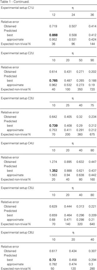
The best estimation of the relative error. Using the procedure of equations 6a and b one can numerically construct exclusion tables for different values of N and obtain the relative error of each non-trivial observ-able Q (equation 9), as Figure 1 graphically shows. Table 1 shows the e.r.e. obtained by this procedure for some experimental setups and the “real” mean relative error coming from the maximum likelihood estimator of

data generated under these different settings. The agreement between the two errors (esti-mated and obtained) is as exact as can be expected for numerical processes. Obviously, such an agreement is independent of Nnt, as

also expected.

Next, we will focus on the approxi-mate direct estimation procedure (step 5b, equation 8). This is because a) we are mainly concerned with an a priori estima-tion of the approximate accuracy a given experimental setup is expected to yield, b) most of the time N is large (N>100) in an LDA, and c) directly solving equation 8 is easier than numerically solving equations 6a and b.

The approximate estimation of the rela-tive error. Table 1 presents relative errors estimated by the approximate procedure

Table 1 - Comparison between the relative error obtained and those predicted both by the best procedure (equations 6a and b) and by the approximate procedure (equation 8) for a series of different experimental designs. The experimental designs were generated by the Strijbosch procedure (Ref. 3; Appendix B, page 947). The number of wells per dilution, η, varied within each experimental setup. Each sub-table also presents the expected number of non-trivial results for each value of η within the experimental setup under analysis. The experimental designs analyzed were:

C1 = [3, 0.15, 0.65, (1:300 to 1:4000)] C2 = [4, 0.10, 0.30, (1:500 to 1:1000)] C3 = [3, 0.70, 0.90, (1:400 to 1:40000)] C4 = [2, 0.10, 0.90, (1:600 to 1:120000)] C5 = [5, 0.35, 0.85, (1:300 to 1:4000)] C6 = [5, 0.15, 0.65, (1:300 to 1:4000)]

where 1) d’, the number of dilutions between P1 and P2; 2) P1; 3) P2, and 4) the upper and the lower boundaries of a frequency range are given within brackets. Thus, [d’, P1, P2, (φ2 to φ1)]. The letters U and L after an

experimental setup stand for the results obtained at the upper and at the lower boundaries of the frequency range, respectively. Notice the fine agreement between the obtained relative error and the predicted ones. On the one hand, such an agreement is independent of the experimental design and the frequency range. On the other hand, such an agreement is jeopardized when the expected non-trivial dilutions comprise a low number of events to be observed. The cases of non-agreement between the predicted and the obtained errors are given in bold (on the “predicted best” lines). This non-agreement is explained by spurious experimental designs resulting in extreme low numbers of non-trivial dilutions associated with high numbers of expected trivial steps. Such a conjunction leads to the emergence of unexpected non-trivial results in putative trivial steps. As an example, consider the experimental setup C3L. The obtained error was 1.529 (italics underlined). This setup comprises 14 dilutions with a putative fraction of negative wells at the lower boundary of the frequency range of Qob(%) = [99.9 99.8 99.7 99.5

99.3 99 98.4 97.7 96.5 94.8 92.3 88.6 83.4 76.2]. Such a Qob leads to only 3 dilutions (underlined) with non-trivial

results when η = 10 wells per dilution (therefore, Nnt = 30). However, there are 110 wells comprising fractions

above 90%, and thus non-trivial results are now expected to emerge within this set of wells (and this is what occurs). When the results are reevaluated after eliminating those 11 trivial steps, the error obtained goes to 1.903, which is now within 5% of the predicted ones. Another problem that emerges at those extremely low numbers of wells comprising the results of an LDA is related to the loss of the nominal confidence interval of the estimator (Chaui-Berlinck JG, unpublished results). However, this is not the subject of this study.

Experimental setup C1U η Experimental setup C1L η

12 24 36 12 24 36

Relative error Relative error

Obtained 0.719 0.507 0.414 Obtained 0.762 0.536 0.436

Predicted Predicted

best 0.8680.8680.8680.8680.868 0.508 0.412 best 0.76 0.521 0.424 approximate 0.952 0.531 0.424 approximate 0.772 0.521 0.425 Expected non-trivial N 36 96 144 Expected non-trivial N 72 192 288 Experimental setup C2U η Experimental setup C2L η

10 20 50 90 10 20 50 90

Relative error Relative error

Obtained 0.614 0.431 0.271 0.202 Obtained 0.574 0.406 0.256 0.191

Predicted Predicted

best 0.7650.7650.7650.7650.765 0.487 0.265 0.188 best 0.557 0.393 0.25 0.186 approximate 0.962 0.532 0.273 0.19 approximate 0.586 0.402 0.252 0.187 Expected non-trivial N 40 100 350 720 Expected non-trivial N 80 160 400 720 Experimental setup C3U η Experimental setup C3L η

10 25 40 75 10 25 40 75

Relative error Relative error

Obtained 0.642 0.405 0.32 0.234 Obtained 1.529 0.926 0.725 0.526

Predicted Predicted

best 0.7390.7390.7390.7390.739 0.408 0.29 0.212 best 2.0512.0512.0512.0512.051 0.9930.9930.9930.9930.993 0.76 0.538 approximate 0.753 0.411 0.291 0.212 approximate 1.984 0.977 0.751 0.533 Expected non-trivial N 70 200 360 675 Expected non-trivial N 30 125 240 600 Experimental setup C4U η Experimental setup C4L η

10 20 40 80 10 20 40 80

Relative error Relative error

Obtained 1.274 0.895 0.632 0.447 Obtained 1.514 1.065 0.75 0.523

Predicted Predicted

best 1.3521.3521.3521.3521.352 0.888 0.621 0.437 best 1.7011.7011.7011.7011.701 1.098 0.745 0.521 approximate 1.563 0.94 0.638 0.442 approximate 1.797 1.122 0.744 0.52 Expected non-trivial N 20 40 80 160 Expected non-trivial N 20 40 120 240 Experimental setup C5U η Experimental setup C5L η

10 20 40 80 10 20 40 80

Relative error Relative error

Obtained 0.629 0.444 0.313 0.221 Obtained 0.953 0.649 0.457 0.323

Predicted Predicted

best 0.659 0.464 0.296 0.209 best 0.9850.9850.9850.9850.985 0.657 0.456 0.321 approximate 0.68 0.471 0.298 0.21 approximate 0.99 0.656 0.455 0.32 Expected non-trivial N 70 140 320 640 Expected non-trivial N 60 160 400 880 Experimental setup C6U η Experimental setup C6L η

10 20 40 10 20 40

Relative error Relative error

Obtained 0.617 0.434 0.307 Obtained 0.655 0.462 0.323

Predicted Predicted

(equation 8) for different experimental set-ups, as well as the mean relative errors coming from the maximum likelihood es-timator of data generated under these dif-ferent settings. Notice that the agreement between the two errors is warranted only when the total non-trivial dilution, Nnt, is

greater than 100. Otherwise, the e.r.e. by the approximate procedure shall overesti-mate such a parameter.

Discussion

Despite the intense use of LDA by immu-nologists in general, its proper employment seems to escape most of them. Two striking problems are the absence of references to how an experimental design is set up (i.e., the range of frequencies that the given setup is prepared to adequately cover) and the use of linear regression by least squares3 _{as the}

estimator of the frequency (in circa 40 to 50% of published studies, our personal ob-servation). Thus, see below five basic state-ments about constraints of the estimation of frequencies in an LDA: 1) in an LDA there is a fixed range of frequencies that can be estimated in a given experimental setup; 2) prior knowledge about a putative range of frequencies to be estimated is a sine qua non

condition in an LDA with the aim of truly determining a certain frequency; 3) such a range should be determined previously, when setting up the experimental design; 4) when the outcome of an experiment falls outside the prior expected range, loss of confidence and power of the estimate occurs, and 5) analysis of the outcome of a particular ex-periment requires programming because there is no good direct analytical LDA esti-mator (e.g., linear regression) and the ad-equate ones are not found in common com-mercial packages.

These features can be found in published

papers about the subject (e.g., 2-4). The empiricist must be aware of these constraints when planning an LDA. Closely related to these problems is the absence of knowledge of what should be expected from a given experimental setup in terms of accuracy. No quantitative prescriptions about the number of wells per dilution (i.e., the number of events to be observed) are found among these constraints (see Introduction). The pres-ent study provides such a quantitative pre-scription, which is based on the relative error of a measure and is thus related to the desired accuracy of such measure. The prescription can be presented as follows: 6) the number of wells in non-trivial steps must be set to match the desired level of accuracy deter-mined a priori.

This putative sixth constraint can be read in either direction, that is, the necessity of increasing the number of wells in a given experiment or the possibility of decreasing such a number in another setting. Let us illustrate these points by means of some “real” problems to be solved. Basically, ac-curacy is expected to be equal to or greater than a given value (thus the relative error is expected to be less than a given value), the number of wells is limited to some maxi-mum N, and the true frequency lies within some range. To these indisputable limits we will add one more: the lower the number of different dilutions to be prepared the less time and energy consuming the experiment will be.

Example 1. The unknown frequency lies in a 20-fold range, d’ = 4, P1 = 0.1, P2 = 0.8 (see Methods). What is the error expected in an experimental setup employing 25 wells per dilution (i.e., η = 25)? What is the gain if

η = 40 instead of 25? The experimental setup will comprise 9 dilutions (d = 9) by the Strijbosch et al. (3) procedure (see Appendix B, page 947 for computation). For the upper

limit in the frequency range, the expected Qob (expected P0(C)) in each dilution (di) is,

respectively, Qob expected (in %) = [73.3

57.3 36.9 16.7 4.1 0.3 0 0 0]. For the lower limit in the frequency range, the expected Qob for each di is, respectively, Qob expected

(in %) = [98.5 97.3 95.1 91.5 85.2 75 59.8 39.7 19.1]. At the upper limit, the number of non-trivial steps expected (for η = 25 wells) comprises dilutions 1 to 5. At the lower limit, the number of non-trivial steps expected comprises dilutions 3 to 9. These numbers of non-trivial expected dilutions are the result of 1/η being equal to 4%, thus excluding dilutions below 4% and above 96% as possible non-trivial dilutions. There-fore, for both extremities in the frequency range, the number of non-trivial dilutions expected, with η = 25, results in Nnt>100

(125 for the upper limit and 175 for the lower one). On this basis, the direct approximate procedure will be employed (equation 8, step 5b). The e.r.e. at the extremities is 0.470 and 0.517, respectively. This represents, roughly speaking, 25% plus and 25% minus around the estimated frequency in a real experiment (e.g., f = φML ± 0.25.φML). When

η is increased to 40 wells, the e.r.e. de-creases to 0.369 and 0.405 at the extremities. One should expect to obtain (approximately) 20% plus and minus around the estimated frequency, representing a 20% increase in accuracy from the η = 25 design. This in-crease is obtained by a 60% inin-crease (15/25) in the number of wells.

Example 2. The relative error is expected to be less than 0.45, N is limited to 300 wells, the expected frequency lies in a 10-fold range. What is best: to set the experiment as A: (d’ = 2, P1 = 0.15, P2 = 0.30, η = 25) or B: (d’ = 4, P1 = 0.10, P2 = 0.60, η = 30)? Notice that setup A concentrates results around the na-dir of the relative error curve (see Figure 1), the so-called “most informative range”. Setup A comprises 12 dilutions (d = 12) and setup B comprises d = 10. As in the above ex-ample, the expected Q at the upper and at the

lower extremities of the frequency range is computed. Then, by computing the expected relative error at the extremities of the fre-quency range in each experimental setup one finds e.r.e. = [0.537 0.355] for A and e.r.e. = [0.412 0.379] for B. Therefore, experimen-tal design B is more consistent with the maximum relative error desired in the entire range of the expected frequencies to be esti-mated. Coincidentally, it is also the less ex-pensive in terms of dilutions to be prepared. All these relevant parameters could be deter-mined beforehand.

Example 3. The relative error is expected to be ≤0.50, the unknown frequency is within a 15-fold range, N is limited to 240 wells. Does a general setting with d’ = 3, P1 = 0.10, P2 = 0.70 and η adjusted as η = integer(N/d) fit the expectations? When the number of cells per dilution is computed under the Strijbosch et al. (3) procedure, one finds that d = 7 and, therefore, η = 34. The expected relative errors for the extremities of the fre-quency range are 0.434 and 0.466. There-fore, such a general setting fits well the expectations of relative errors of less than 0.50 for a 15-fold range of the unknown frequency.

Example 4. Consider a problem similar to the above example, but with the unknown frequency restricted to a 5-fold range. The experimental setup is now reduced to 5 dilu-tions, and thus η = 48. Accuracy increases, as indicated by the e.r.e. of 0.361 and 0.413 at the extremities.

of these determinations are to be made or in terms of relaxing the relative error expected). The use of dilutions related to each other by a power rule (e.g., y(n) = Z(n-1) .y(1)) is given

as an inadequate experimental setup proce-dure by Fazekas de St. Groth (2). When one computes the relationship between the num-ber of cells in each dilution of the experimental setup given in example 5 each step is found to contain approximately 1.862 times the num-ber of cells of the preceding one (i.e., the power scaling factor Z = 1.862). In fact, a given composition of d’, P1 and P2 under the Strijbosch et al. (3) procedure generates a power scaling factor (notice that the frequency range does not matter for such an underlying rule). In example 1, the power scaling factor is 1.792. In example 2, the power scaling factor is 1.255 for setup A and 1.457 for setup B. Despite an underlying power scaling factor, it is possible to attain relative errors at a desired level, contradicting Fazekas de St. Groth’s statement about the power rule. What this investigator means must be read as “one should

not employ a fixed power scaling factor for every frequency determination”. Strijbosch et al. (3) provide an easy way to find the adequate power scaling factor. This study provides an easy way to evaluate the accuracy such a scaling factor shall yield under empirical con-ditions.

Conclusion

This study provides an easy way to esti-mate beforehand the relative error (i.e., the accuracy) of an LDA experimental setup. This can be done following steps 1, 2, 3, 4, 5b and 6 in Methods and in equations 7, 8 and 9, when the expected number of non-trivial dilutions4 _{is large (i.e., non-trivial}

di-lutions comprise, overall, more than 100 wells). When such an expected number is less than 100, care must be taken because both the relative error and the nominal con-fidence level of the estimator can be wrongly estimated.

References

1. Taswell C (1981). Limiting dilution assays for the determination of immunocompe-tent cell frequencies. I. Data analysis.

Journal of Immunology, 126: 1614-1619. 2. Fazekas de St. Groth S (1982). The

evalua-tion of limiting diluevalua-tion assays. Journal of Immunological Methods, 49: R11-R23. 3. Strijbosch LWG, Buurman WA, Does

RJMM, Zinken PH & Groenewegen G (1987). Limiting dilution assays: experi-mental design and statistical analysis.

Journal of Immunological Methods, 97:

133-140.

4. Cobb L, Cyr L, Schmehl MK & Bank HL (1989). Comparison of statistical methods for the analysis of limiting dilution assays.

In Vitro Cellular and Developmental Biol-ogy, 25: 76-81.

5. Schmehl MK, Cobb L & Bank HL (1989). Power analysis of statistical methods for comparing treatment differences from limiting dilution assays. In Vitro Cellular and Developmental Biology, 25: 69-75. 6. Burleson JÁ, Binder TA & Goldschneider I

(1993). Use of logistic regression in com-paring multiple limiting dilution analyses of antigen-reactive T cells. Journal of Im-munological Methods, 159: 47-52. 7. Vuolo JH (1996). Fundamentos da Teoria

dos Erros. 2nd edn. Editora Edgard Blü-cher Ltda., São Paulo.

8. Sokal RR & Rohlf FJ (1995). Biometry: the Principles and Practice of Statistics in Bio-logical Research. 3rd edn. W.H. Freeman

and Company, New York.

4_{Non-trivial dilutions are those in which the expected number of positive wells in the dilution is different from}

Appendix A

Suppose η (e.g., 100) events were observed and the resulting probability of positive events (i.e., positive outcomes/η) among these events is p1 (e.g., p1 = 0.1). Suppose another set of η events resulted in another p2 (e.g., p2 = 0.4). What one should expected if, instead of observing two separate sets of η events, one had observed one set of 2.η events? These being independent events, the conjunction of p1 and p2 is the unbiased expectation one should have to obtain at the 2.η level. This means:

Appendix B

The first step in the Strijbosch et al. (3) procedure is to determine the frequency range to be evaluated, φ1 (the lower boundary) and φ2 (the upper boundary, 0<φ1≤φ2<1). Then, the

two boundaries (P1 and P2) in the fraction of negative wells (i.e., 0<P1<P2<1) and the number of dilutions d’ to be found between P1 and P2 are set. The computation below (taken from Ref. 3) shows how many dilutions and what number of cells per dilution are to be employed to satisfy the conditions established a priori:

( )

(

) (

_{) ( )}

(

)

(

)

2 c

1

0.5 1 J

1

1 2

j 1 j 1

1 d

J=d +INTEGER log

c

x

ln P1

ln P2

x

x c , j

2, 3, ..., J

where

ln P1

c=

ln P2

−

−

′



φ



′

_

_

_φ

_

_









=



⋅

⋅

_{φ ⋅φ}











= ⋅

=













In the numerical example above, the expected number of positive events is 200.(0.04 + 0.03 + 0.18) = 50. Obviously, this ends up as the mean between p1 and p2, (p1 + p2)/2. The extension to any number X of subsets of ηi events is straightforward: Prob(X.η) =

mean(Prob(ηi)).

(

)

(2 )

p1 (1 p2) (1 p1) p2 expected number of positive events 2 p1 p2

2 2

⋅η

  ⋅ −   − ⋅ 

= ⋅ η⋅_ ⋅ +_{   }+ _