HESSD
12, 4997–5053, 2015Integrated water system simulation
Y. Y. Zhang et al.
Title Page
Abstract Introduction
Conclusions References
Tables Figures
◭ ◮
◭ ◮
Back Close
Full Screen / Esc
Printer-friendly Version Interactive Discussion
Discussion
P
a
per
|
Discussion
P
a
per
|
Discussion
P
a
per
|
Discussion
P
a
per
|
Hydrol. Earth Syst. Sci. Discuss., 12, 4997–5053, 2015 www.hydrol-earth-syst-sci-discuss.net/12/4997/2015/ doi:10.5194/hessd-12-4997-2015
© Author(s) 2015. CC Attribution 3.0 License.
This discussion paper is/has been under review for the journal Hydrology and Earth System Sciences (HESS). Please refer to the corresponding final paper in HESS if available.
Integrated water system simulation by
considering hydrological and
biogeochemical processes: model
development, parameter sensitivity and
autocalibration
Y. Y. Zhang1, Q. X. Shao2, A. Z. Ye3, H. T. Xing1,4, and J. Xia1
1
Key Laboratory of Water Cycle and Related Land Surface Processes, Institute of Geographic Sciences and Natural Resources Research, Chinese Academy of Sciences, Beijing, 100101, China
2
CSIRO Digital Productivity Flagship, Leeuwin Centre, 65 Brockway Road, Floreat Park, WA 6014, Australia
3
College of Global Change and Earth System Science, Beijing Normal University, 100875, Beijing, China
4
HESSD
12, 4997–5053, 2015Integrated water system simulation
Y. Y. Zhang et al.
Title Page
Abstract Introduction
Conclusions References
Tables Figures
◭ ◮
◭ ◮
Back Close
Full Screen / Esc
Printer-friendly Version Interactive Discussion
Discussion
P
a
per
|
Discussion
P
a
per
|
Discussion
P
a
per
|
Discussion
P
a
per
|
Received: 1 April 2015 – Accepted: 29 April 2015 – Published: 22 May 2015
Correspondence to: Y. Y. Zhang ([email protected])
HESSD
12, 4997–5053, 2015Integrated water system simulation
Y. Y. Zhang et al.
Title Page
Abstract Introduction
Conclusions References
Tables Figures
◭ ◮
◭ ◮
Back Close
Full Screen / Esc
Printer-friendly Version Interactive Discussion
Discussion
P
a
per
|
Discussion
P
a
per
|
Discussion
P
a
per
|
Discussion
P
a
per
|
Abstract
Integrated water system modeling is a reasonable approach to provide scientific un-derstanding of severe water crisis faced all over the world and to promote the imple-mentation of integrated river basin management. Time Variant Gain Model (TVGM), which is a classic hydrological model, is based on the complex Volterra nonlinear
for-5
mulation and has gotten good performance of runoff simulation in numerous basins.
However, TVGM is disadvantageous to predict other water-related components. In this study, TVGM was extended to an integrated water system model by coupling multiple water-related processes in hydrology, biogeochemistry, water quality and ecology, and considering the interference of human activities. The parameter sensitivity and
autocal-10
ibration modules were also developed to improve the simulation efficiency. The Shaying River Catchment, which is the largest, highly regulated and heavily polluted tributary in the Huai River Basin of China, was selected as the study area. The key water related components (e.g., runoff, water quality, nonpoint source pollutant load and crop yield) were simulated. The results showed that the extended model produced good simulation
15
performance of most components. The simulated daily runoffseries at most regulated
and less-regulated stations matched well with the observations. The average values of correlation coefficient and coefficient of efficiency between the simulated and
ob-served runoffs were 0.85 and 0.70, respectively. The simulations of both low and high
flow events were improved when the dam regulation was considered except the low
20
flow simulation at Zhoukou and Huaidian stations. The daily ammonia-nitrogen (NH4
-N) concentration, as a key index to assess water quality in China, was well captured with the average correlation coefficient of 0.67. Furthermore, the nonpoint source NH4
-N load and corn yield were simulated for each administrative region and the results were reasonable in comparison with the data from the official report and the statistical
25
HESSD
12, 4997–5053, 2015Integrated water system simulation
Y. Y. Zhang et al.
Title Page
Abstract Introduction
Conclusions References
Tables Figures
◭ ◮
◭ ◮
Back Close
Full Screen / Esc
Printer-friendly Version Interactive Discussion
Discussion
P
a
per
|
Discussion
P
a
per
|
Discussion
P
a
per
|
Discussion
P
a
per
|
1 Introduction
Severe water crises are global issues emerged in the rapid development of social econ-omy, including flooding (Milly et al., 2002; Schiermeier et al., 2011), water shortages (Pimentel et al., 2004; Wilhite et al., 2005), water pollution (Jordan et al., 2014; Zhou et al., 2014) and ecological degradation (Revenga et al., 2000; Vörösmarty et al., 2010).
5
These issues are hindering regional equitable development by compromising the sus-tainability of vital water resource and ecosystem (Gleick, 1997). It is impossible to ad-dress these water-related problems within a single scientific discipline (e.g., hydrology, hydraulics, water quality or aquatic ecology) due to the complicated interconnections among the physical, chemical and ecological components of an aquatic ecosystem
10
(Kindler, 2000; Biswas, 2004; Paola et al., 2006). The integrated river basin manage-ment might be a sensible solution at basin scale by the coordinated managemanage-ment of water resources among the social-economy, water quality and ecosystems (Rahaman and Varis, 2005; Hering et al., 2012). Integrated water system modeling is a reasonable practice to simultaneously simulate water related components (flow regimes, nutrient
15
loss, sediment and water pollution), and also an effective tool to support water resource allocation, environmental flow management and river restoration (Arthington, 2012).
Integrated water system modeling has gained popularity due to the rapid develop-ment of water related sciences, computer sciences and earth observation technolo-gies in the last decades. The hydrological cycle has been widely accepted as a critical
20
linkage among physical (e.g., runoff), biogeochemical (e.g., nutrient, water quality) and ecological processes (e.g., plant growth), energy fluxes at basin scale (Wigmosta et al., 1994; Singh and Woolhiser, 2002; Burt and Pinay, 2005). For example, the physiologi-cal and ecologiphysiologi-cal processes of vegetation affect evapotranspiration, soil moisture dis-tribution and infiltration, and nutrients absorption and movement. On the contrary, soil
25
HESSD
12, 4997–5053, 2015Integrated water system simulation
Y. Y. Zhang et al.
Title Page
Abstract Introduction
Conclusions References
Tables Figures
◭ ◮
◭ ◮
Back Close
Full Screen / Esc
Printer-friendly Version Interactive Discussion
Discussion
P
a
per
|
Discussion
P
a
per
|
Discussion
P
a
per
|
Discussion
P
a
per
|
causes at the basin scale by coupling all these processes and capturing the interac-tions and feedbacks between individual cycles. Furthermore, multidisciplinary research
provides an effective way to make possible breakthroughs in water system modeling
by integrating the mature basic theories of water-related disciplines (e.g., accumulated temperature law for phenological development, Dacy’s law for groundwater flow,
Saint-5
Venant Equation for surface flow, balance equation for mass and momentum, Richards equation for unsaturated zone, Horton theory for infiltration, Penman–Monteith equa-tion for evapotranspiraequa-tion), and abundant data sources (e.g., high resoluequa-tion of spatial information data: DEM, land use and crop distribution, chemical and isotopic data from field experiment) (Singh and Woolhiser, 2002; Kirchner, 2006).
10
Several models have been developed based on the mature models of different
dis-ciplines since the 1980s (Singh and Woolhiser, 2002). Due to the complexity of the integrated system, most of existing models focus on one or two major water related pro-cesses, depending on the model orientation (e.g., hydrology, water quality, and
biogeo-chemistry). The hydrological models emphasize on the rainfall–runoffrelationship and
15
link with several dominating water quality and biogeochemical processes. As a result, these models usually have satisfactory performance in major hydrological processes. Examples of widely accepted models include TOPMODEL (Beven and Kirkby, 1979), SHE (Abbott et al., 1986), HSPF (Bicknell et al., 1993), VIC (Liang et al., 1994) and ANSWERS (Bouraoui and Dillaha, 1996). The water quality models focus on the
mi-20
gration and transformation processes of pollutants in water bodies. The models can get the detailed spatial and temporal variations of water quality variables in river system by adopting multi-dimensional dynamic equation, but are difficult to simulate the overland processes of water and pollutants. The typical models are WASP (Di Toro et al., 1983), QUAL2E (Brown and Barnwell, 1987), EFDC (Hamrick, 1992). The biogeochemistry
25
path-HESSD
12, 4997–5053, 2015Integrated water system simulation
Y. Y. Zhang et al.
Title Page
Abstract Introduction
Conclusions References
Tables Figures
◭ ◮
◭ ◮
Back Close
Full Screen / Esc
Printer-friendly Version Interactive Discussion
Discussion
P
a
per
|
Discussion
P
a
per
|
Discussion
P
a
per
|
Discussion
P
a
per
|
ways in the basin. The examples are EPIC (Sharpley and Williams, 1990), DNDC (Li et al., 1992).
SWAT is a typical integrated water system model, which simulates most of water re-lated processes over long time periods at large scales and has been widely accepted (Arnold et al., 1998). Its model structure and functions are considered as a landmark in
5
the field of water system modeling. However, not all of water related processes could be well captured in practice due to the applicability and inaccurate descriptions of some modules, such as daily simulations of extreme flow events (Borah and Bera, 2004), soil nitrogen and carbon (Gassman et al., 2007), the performance in regulated basins (Zhang et al., 2012). Particularly, SWAT applies two alternative approaches to
simu-10
late surface runoff, e.g., the empirical Soil Conservation Service (SCS) curve number
method and the conceptual Green–Ampt infiltration model. The SCS equation is usu-ally given priority, but the applicability of curve number is questioned (Rallison and Miller, 1981). The Green–Ampt infiltration model is usually limited to simulate flow events at micro temporal and spatial scales (Brakensiek, 1977; King et al., 1999).
Fur-15
thermore, it is much more difficult for SWAT to capture the complicated dynamic
pro-cesses of soil nitrogen and carbon accurately in comparison with other biochemistry models (Gassman et al., 2007). Polhert et al. (2006, 2007) was extended SWAT with algorithms from DNDC (SWAT-N), and found that SWAT-N could be used for monthly and weekly prediction of nitrate load, but should be avoided for daily prediction.
20
Time Variant Gain Model (TVGM) is a lumped hydrological model, which was
pro-posed by Xia (1991) based on the hydrological data from many different scales basins
all over the world. In TVGM, the rainfall–runoffrelationship is considered to be nonlinear with surface runoffcoefficient varying over time and being affected significantly by an-tecedent soil moisture (Xia et al., 1991). TVGM has strong mathematics basis because
25
HESSD
12, 4997–5053, 2015Integrated water system simulation
Y. Y. Zhang et al.
Title Page
Abstract Introduction
Conclusions References
Tables Figures
◭ ◮
◭ ◮
Back Close
Full Screen / Esc
Printer-friendly Version Interactive Discussion
Discussion
P
a
per
|
Discussion
P
a
per
|
Discussion
P
a
per
|
Discussion
P
a
per
|
the impact of human activities and climate change on runoff, and got good simulation
performance (Xia et al., 2005; Wang et al., 2009). However, DTVGM was confined to the studies of hydrological cycle and could not be applied to the integrated river basin management due to the lack of considering other water-related processes, such as the water quality processes, ecological processes, soil biogeochemical processes.
5
The objective of this study is to extend DTVGM to an integrated water system model by considering hydrological, biogeochemical, water quality and ecological processes, and the prevalent regulation by water projects, with the aim to meet the demand of the integrated river basin management. The model framework is developed based on the interchange among the processes of water and nutrient depicted by several robust
10
models. The parameter analysis module is also included in our programming codes. The extended model is expected to capture the spatial and temporal variations of sev-eral key water-related components (e.g., flow regimes, nonpoint source pools of nutri-ents, water quality variables in water body and crop yield) in complex basins.
2 Methods and material
15
2.1 Model framework
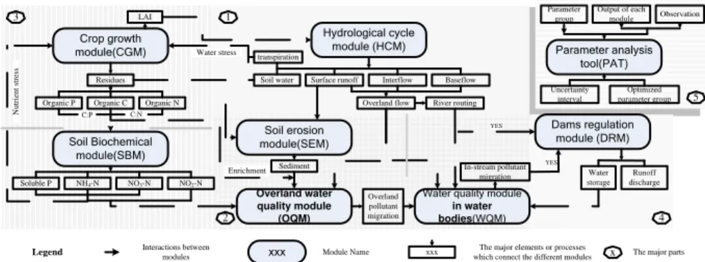
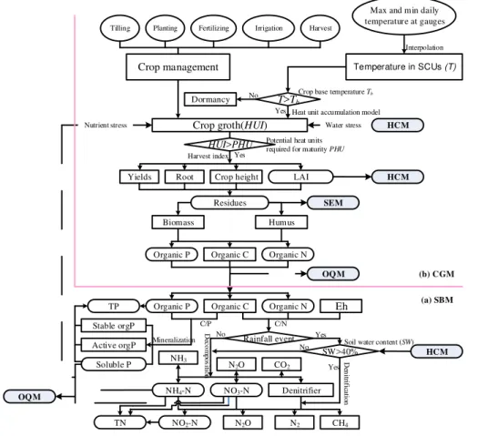
The proposed model includes seven major modules, named as hydrological cycle mod-ule (HCM), soil biochemical modmod-ule (SBM), crop growth modmod-ule (CGM), soil erosion module (SEM), overland water quality module (OQM), water quality module of water bodies (WQM) and dam regulation module (DRM). Parameter analysis tool (PAT) is
20
a useful tool for model calibration and is independent from other modules. The exterior
exchange components connecting different modules are given in Fig. 1. More detailed
description of each module and its interactions with other modules are given in the following individual Sects. from 2.1.1 to 2.1.6. The main equations of each process are deferred to the appendix and supplementary material section for readers who are
25
HESSD
12, 4997–5053, 2015Integrated water system simulation
Y. Y. Zhang et al.
Title Page
Abstract Introduction
Conclusions References
Tables Figures
◭ ◮
◭ ◮
Back Close
Full Screen / Esc
Printer-friendly Version Interactive Discussion
Discussion
P
a
per
|
Discussion
P
a
per
|
Discussion
P
a
per
|
Discussion
P
a
per
|
The extended model is based on the hypothesis that the cycles of water and nu-trients (N, P and C) are inseparable and act as the critical linkages among all the modules. Firstly, several key hydrological components simulated by hydrological mod-ule are critical linkages among all the modmod-ules, such as evapotranspiration, soil water moisture, flow (Sect. 2.1.1). Secondly, soil biochemical processes determine the
nutri-5
ent load absorbed in the crop growth process (CGM) and migrated into water bodies as the nonpoint pollutant source (OQM and WQM). The complicated nutrient processes in the soil profiles are described in detail to improve the simulation of water quality processes in responding to agricultural management (Sect. 2.1.2). Thirdly, the hydro-logical module also provides a function to describe the spatial relationship among the
10
spatial calculation units, in order to help the simulation of the overland and in-stream movement of water and nutrient at the basin scale (Sects. 2.1.1 and 2.1.3). Therefore, the proposed model takes full advantages of powerful interconnection and simulation functions of hydrological model at large spatial scale, elaborative description of nu-trient vertical movement in soil layers of ecological model at field scale and nunu-trient
15
movement in river networks of water quality model.
2.1.1 Hydrological cycle module (HCM)
The calculation of surface runoff yield is the core of hydrological simulation and has
close relationships with many other processes. The surface runoff yields are
calcu-lated by TVGM separately for different landuse area including forest, grassland, water,
20
urban, unused land, paddy land and dry land. The potential evapotranspiration is cal-culated using Hargreaves method (Hargreaves and Samani, 1982) because it only uses the daily maximum and minimum temperature data which are widely available. The actual plant transpiration is expressed as a function of potential evapotranspiration and leaf area index while the soil evaporation is expressed as a function of potential
25
stor-HESSD
12, 4997–5053, 2015Integrated water system simulation
Y. Y. Zhang et al.
Title Page
Abstract Introduction
Conclusions References
Tables Figures
◭ ◮
◭ ◮
Back Close
Full Screen / Esc
Printer-friendly Version Interactive Discussion
Discussion
P
a
per
|
Discussion
P
a
per
|
Discussion
P
a
per
|
Discussion
P
a
per
|
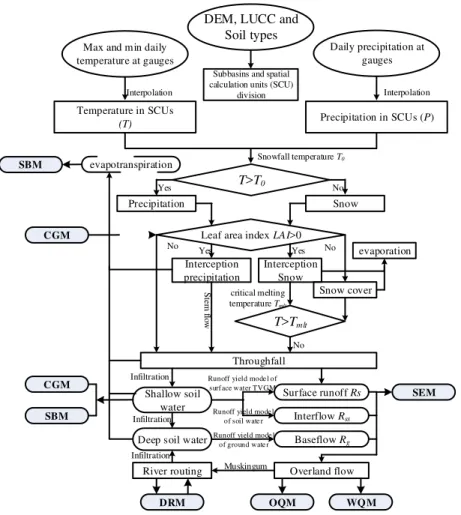
age routing methodology (Neitsch et al., 2011). The Muskingum method or kinetic wave equation is used for river flow routing.
A flowchart is given in Fig. 2, from which it can be seen that shallow soil water from the hydrological cycle module is one of the major factors connecting the crop growth module (to control crop growth) and the soil biochemical module (to control vertical
5
migration and reaction of nutrients in the soil profiles). Plant transpiration is also linked to the soil biochemical module (to provide energy for vertical migration of nutrients in the soil profiles). The surface runoffis linked to the soil erosion and the overland flow is connected to the overland water quality modules (to drive migration of nutrients and
sediment along flow paths) and water quality module for runoffrouting in water bodies
10
(rivers and lakes). Moreover, the hydrological cycle module calculates inflow of dam or sluice for the dam regulation module.
2.1.2 Ecological process modules
Ecosystem is one of the decisive components to the hydrological cycle and the pol-lutant migration and transportation. The model incorporates the water cycle, nutrient
15
cycles and crops growth, as well as their key linkages. The ecological process mod-ules contain SBM and CGM.
Soil biochemical module (SBM)
The soil biochemical module simulates the key processes of Carbon (C), Nitrogen (N) and Phosphorus (P) dynamics in the soil profiles, including decomposition,
mineraliza-20
tion, immobilization, nitrification, denitrification, plant uptake and leaching. C constrains the decomposition and denitrification of N and P. Different forms of nutrients (N and P) outputted from the soil biochemical module are connected to the crop growth module as the nutrient constraints of crop growth, and to the overland water quality module as the main nonpoint sources of pollutant to water bodies (Fig. 3a). The daily step
25
bio-HESSD
12, 4997–5053, 2015Integrated water system simulation
Y. Y. Zhang et al.
Title Page
Abstract Introduction
Conclusions References
Tables Figures
◭ ◮
◭ ◮
Back Close
Full Screen / Esc
Printer-friendly Version Interactive Discussion
Discussion
P
a
per
|
Discussion
P
a
per
|
Discussion
P
a
per
|
Discussion
P
a
per
|
geochemical processes of C and N in the soil profile at field scale, which is variable according to the crop pattern in the actual situation (Li et al., 1992). The major pro-cesses of soil P cycle are simulated based on the study of Horst et al. (2001). The soil profile is divided into three layers, e.g., surface (0–10 cm), and user defined upper and lower layer, all of which are consistent with the soil layers of hydrological cycle module
5
in order to exchange the values of linkages (e.g., soil water) among different modules smoothly.
Soil C and N cycle.The decomposition and other oxidation processes are the dominant microbial processes in the aerobic condition, while the denitrification process occurs under anaerobic condition.
10
– Decomposition.There are three conceptual organic C pools: the decomposable residue pool, microbial biomass pool and a stable pool (humus). Every pool con-tains resistant and labile components. Additionally, the residue pool concon-tains a very labile component. The decomposition of each C pool is treated as the first-order decay process with the individual decomposition being modified by soil
15
temperature and moisture, clay content and the C : N ratio. Carbon dioxide (CO2),
released from soil organic carbon (SOC), is calculated as a constant fraction of the C undergoing decomposition of three C pools. When the soil water filled pore space (WFPS) in the surface soil layer is increased over 55 % by precipitation and/or irrigation, the decomposition process will pause and the denitrification
pro-20
cess will start. The decomposition will start again and denitrification will stop when WFPS is below 55 % or the substrates are used up. The details of SOC pool struc-ture are described in Li et al. (1992).
– Nitrogen transformation during decomposition. The major simulated processes of decomposition under aerobic condition are mineralization, immobilization,
am-25
monia (NH3) volatilization and nitrification. Ammonium (NH+4) is mineralized from organic N pool when SOC flows from C pool with lower C : N ratio into C pool with
HESSD
12, 4997–5053, 2015Integrated water system simulation
Y. Y. Zhang et al.
Title Page
Abstract Introduction
Conclusions References
Tables Figures
◭ ◮
◭ ◮
Back Close
Full Screen / Esc
Printer-friendly Version Interactive Discussion
Discussion
P
a
per
|
Discussion
P
a
per
|
Discussion
P
a
per
|
Discussion
P
a
per
|
N (NO−3 and NH+4) is immobilized into soil organic N pool, when SOC flows from the higher C : N ratio C pools into the lower C : N ratio C pools. Model assumes that the flow rate of SOC from the higher C : N ratio C pool to the lower C pool (higher C : N ratio C pool decomposition) will reduce to an allowable level to meet the available mineral N if the mineral N is not enough. NH3 volatilization is
con-5
trolled by the simulated NH+4 concentration, clay content, pH, soil moisture and temperature. NH+4 is microbial oxidized to NO3- and nitrous oxide (N2O) which
emit into the air as a gaseous intermediate matter during nitrification. The propor-tion of N2O is controlled by NH+4 concentration, pH, temperature, moisture in the
soil layer.
10
– Denitrification.The denitrification process occurs when WFPS is greater than the threshold (55 %) during rainfall or irrigation events. The generally recognized
re-duction sequence in denitrification is NO−3 → NO2 → NO → N2O → N2. The
denitrification rate correlates with denitrifier biomass, moisture, pH, temperature and NO−3 concentration in the soil layer. The denitrifier biomass is estimated with
15
the growth and dead rate of denitrifier which is controlled by dissolved soil or-ganic C, soil moisture and temperature. The C and N from dead cells are added to the pools of immobilized C and N which no longer participate in the dynamic processes. The consumption rate of soluble C depends on the biomass, relative growth rate, and the maintenance coefficients of the denitrifier populations. The
20
daily emission rates of greenhouse gases (N2O, NO and N2) are related to the
adsorption coefficients of gases in soils and the air filled porosity of the soil. But
N2O and NO emissions are neglected because of the low diffusion rates in soil
water if WFPS is over 90 %.
Soil P cycle. Six P pools are considered, e.g., three organic pools (stable and
ac-25
con-HESSD
12, 4997–5053, 2015Integrated water system simulation
Y. Y. Zhang et al.
Title Page
Abstract Introduction
Conclusions References
Tables Figures
◭ ◮
◭ ◮
Back Close
Full Screen / Esc
Printer-friendly Version Interactive Discussion
Discussion
P
a
per
|
Discussion
P
a
per
|
Discussion
P
a
per
|
Discussion
P
a
per
|
sidered in Horst et al. (2001) and Neitsch et al. (2011), through modeling the P release from fertilizer, manure, residue, microbial biomass and humic substances, P sorption by plant uptake, and P transportation by sediment and overland flow.
Crop growth module (CGM)
The crop growth module is developed based on EPIC crop growth model (Hamrick,
5
1992), which applies the concept of daily accumulated heat units on phenological crop development, Monteith’s approach for potential biomass, harvest index for partitioning grain yield, and stress adjustments for water, temperature and nutrient (N and P) avail-ability in the root zone of the soil profile. It simulates total dry matter, leaf area index, root depth and density distribution, harvest index, nutrient uptake, etc (Willians et al.,
10
1989; Sharpley and Williams, 1990). The crop respiration and photosynthesis drive the vertical movement of water and nutrient. In the crop growth module, the output of leaf area index is the main factor connecting the hydrological cycle module (to control the transpiration), and the crop residue left in the fields is the main source of organic matters (C, N and P) connecting to the soil biochemical module for soil biochemical
15
processes, to the overland water quality module, and to the soil erosion module as one of the five constraint factors (Fig. 3b).
2.1.3 Water quality process modules
The water quality process modules focus on the migration and transformation of water quality variables (e.g., sediment, different forms of nutrients, chemical oxygen demand:
20
COD) along with the water movement in the land surface and river systems. The main modules are the soil erosion module for the sediment yield, the overland water qual-ity module for the nonpoint source pollutant loss and migration from the soil layers to water bodies (rivers or lakes), and the water quality module for the migration and transformation of pollutants in the water bodies (point and non-point source loads).
HESSD
12, 4997–5053, 2015Integrated water system simulation
Y. Y. Zhang et al.
Title Page
Abstract Introduction
Conclusions References
Tables Figures
◭ ◮
◭ ◮
Back Close
Full Screen / Esc
Printer-friendly Version Interactive Discussion
Discussion
P
a
per
|
Discussion
P
a
per
|
Discussion
P
a
per
|
Discussion
P
a
per
|
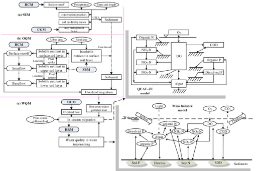
Soil erosion module (SEM)
The soil erosion by precipitation is estimated using the improved USLE equation
(On-stad and Foster, 1975) based on runoffoutputted from the hydrological cycle module,
crop management factor outputted from the crop growth module. The soil erosion mod-ule simulates sediment load for the overland water quality modmod-ule to provide the carrier
5
for the migration of insoluble organic matters along overland transport paths and water bodies (Fig. 4a).
Overland water quality module (OQM)
This module is to simulate the overland loss and migration load of nonpoint source pollutant (e.g., sediment, insoluble and soluble nutrients, COD) for the water quality
10
module of water bodies (Fig. 4b). Their main sources are the nutrient loss from the soil layers and urban area, the farm manure from living and livestock breeding in the rural area. The nutrient loss from the soil layers, as the primary nonpoint source in most catchments, is determined by the overland flow and sediment yield (Williams et al., 1989; Neitsch et al., 2011) and the other sources are estimated using the export
co-15
efficient method (Johnes, 1996; Lin, 2004). The overland migration processes contain
the soluble pollutant migration with overland flow and the insoluble pollutant migration with sediment. All of these processes take place along the overland transport paths.
Water quality module of water bodies (WQM)
There are point and nonpoint sources of pollutant discharged into water bodies in the
20
basins. The point source load is the direct input of our proposed model, including the observed urban inhabitant and industrial sewage discharged into river network while the nonpoint source load is simulated by the overland water quality module.
Two modules are designed for different types of water bodies, e.g., the in-stream wa-ter quality module and the wawa-ter quality module of wawa-ter impounding (reservoir or lake).
HESSD
12, 4997–5053, 2015Integrated water system simulation
Y. Y. Zhang et al.
Title Page
Abstract Introduction
Conclusions References
Tables Figures
◭ ◮
◭ ◮
Back Close
Full Screen / Esc
Printer-friendly Version Interactive Discussion
Discussion
P
a
per
|
Discussion
P
a
per
|
Discussion
P
a
per
|
Discussion
P
a
per
|
The enhanced stream water quality model (QUAL-2E) (Brown and Barnwell, 1987), as a comprehensive and versatile stream model, is adopted to simulate the longitudinal movement and transformation of water quality variables in the branch stream systems. The model is centered at dissolved oxygen (DO) and can simulate up to 15 water
qual-ity variables including temperature, DO, sediment, different forms of nutrient (N and
5
P), COD (Fig. 4c). The model is solved at the subbasin scale rather than the fine grid scale. The water quality outputs are linked to the dam regulation module to provide upper water quality boundary of dams or sluices. The water quality module of water impounding assumes that water body is at the steady state and focuses on the verti-cal interaction of water quality. The main processes are the water quality degradation,
10
settlement, resuspension and decay in the sediment.
2.1.4 Dam regulation module (DRM)
The dams or sluices highly disturb flow regimes and associated water quality processes in most river networks (Zhang et al., 2013). The dam or sluice regulation should be con-sidered in the water system models. The dam regulation module provides hydrological
15
boundaries (e.g., water storage, runoff) regulated by dams or sluices to the hydrolog-ical cycle module for flow routing and to the water quality module of water bodies for pollutant migration.
In this module, three methods are proposed for calculating water storage and outflow of dams or sluices, i.e., measured outflow, controlled outflow with target water storage,
20
and the relationship between outflow and water storage volume (Zhang et al., 2013). The first method requires users to provide the measured outflow series during the sim-ulation period. The second method simplifies the regsim-ulation rule of dam or sluice for the long-term analysis by assuming that water is stored according to the usable water level during the non-flooding season and the flood control level during the flooding season
25
HESSD
12, 4997–5053, 2015Integrated water system simulation
Y. Y. Zhang et al.
Title Page
Abstract Introduction
Conclusions References
Tables Figures
◭ ◮
◭ ◮
Back Close
Full Screen / Esc
Printer-friendly Version Interactive Discussion
Discussion
P
a
per
|
Discussion
P
a
per
|
Discussion
P
a
per
|
Discussion
P
a
per
|
method is proposed based on relationship among water level, water surface area, stor-age volume and outflow according to the design data of dam, or long-term observed data (Appendix C).
2.1.5 Multi-scale solution
Spatial heterogeneities of basin attributes and inconsistent reaction times of diff
er-5
ent processes result in the multiple spatial and temporal scales of hydrological, water quality and ecological processes (Blöschl and Sivapalan, 1995; Sivapalan and Kalma, 1995; Singh and Woolhiser, 2002; Lohse et al., 2009). For the spatial scale, three lev-els of spatial calculation units are designed in the model, i.e. subbasin unit, landuse unit and crop unit from largest to smallest. These units are the minimum polygons with
10
similar hydrological properties, landuse type and agriculture crop cultivation pattern, respectively. The subbasins are defined on the basis of DEM, the position of gauges and water projects (dams or sluices), and are used in the hydrological cycle module (e.g., flow routing in both land and in-stream), overland water quality module, water quality module of water bodies and dam regulation module. Seven specific landuse
15
units of each subbasin are partitioned by the landuse classification (e.g., forest, grass-land, water, urban, unused grass-land, paddy land and dry land). The related modules are the hydrological cycle module (e.g., water yield, infiltration, interception and evapotranspi-ration) and soil erosion module. Moreover, several specific landuse units (paddy land and dry land, forest, grassland), where agricultural activities usually occur, are divided
20
further into crop units for detailed analysis of the impact of agricultural management on water and nutrient cycles. In the current version of the model, ten specific categories of crop units are divided for these four landuse units, i.e. fallow for all these landuse units; grass for grassland unit; fruit tree and non-economic tree for forest unit; early rice and late rice for paddy unit; spring wheat, winter wheat, corn, and mixed dry crop
25
HESSD
12, 4997–5053, 2015Integrated water system simulation
Y. Y. Zhang et al.
Title Page
Abstract Introduction
Conclusions References
Tables Figures
◭ ◮
◭ ◮
Back Close
Full Screen / Esc
Printer-friendly Version Interactive Discussion
Discussion
P
a
per
|
Discussion
P
a
per
|
Discussion
P
a
per
|
Discussion
P
a
per
|
landuse unit scale, or subbasin scale based on the area percentage of different units, respectively.
For the temporal scale, the time step of our proposed model is one day because most simulated processes are usually considered to take place at daily scale (Lohse et al.,
2009). The linear or nonlinear aggregating functions are used to transform different
5
time scales to the daily scale (Vinogradov et al., 2011), such as exponential relation for the flow infiltration and overland flow routing processes, soil erosion processes (A5, A6 and S32), accumulative relation for the crop growth process (S7 in the Supplement).
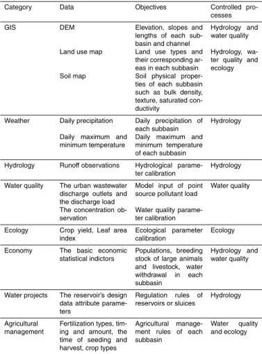
2.1.6 Basic datasets and spatial delineation
The indispensable datasets of the proposed model are GIS data (DEM, soil physical
10
and chemical properties, land use and crop types), daily meteorological data series (precipitation, maximum and minimum air temperature), social and economic data se-ries (population and livestock number in rural area, chemical fertilizer types, amount and cultivation methods, water withdrawal and point source pollutant load), dam at-tribute data (water storage capacities of dead, usable, flood control and maximum flood
15
levels and the corresponding water surface areas). Several monitoring data series are also needed for model calibration, such as runoffand water quality series at river sec-tions, soil water moisture and crop yield at the field scale. All the datasets and their usages are given in Table 1.
The hydrological toolset of Arc GIS platform are used to delineate all the spatial
cal-20
culation units and river system based on DEM, landuse data. The subbasin attributes (e.g., subbasin area, land surface slope and slope length) and flow routing relationship between subbasins are also obtained during this procedure.
2.2 Parameter analysis and calibration
Parameter sensitivity analysis and auto-calibration are critical steps for the
applica-25
espe-HESSD
12, 4997–5053, 2015Integrated water system simulation
Y. Y. Zhang et al.
Title Page
Abstract Introduction
Conclusions References
Tables Figures
◭ ◮
◭ ◮
Back Close
Full Screen / Esc
Printer-friendly Version Interactive Discussion
Discussion
P
a
per
|
Discussion
P
a
per
|
Discussion
P
a
per
|
Discussion
P
a
per
|
cially for the integrated water system models (Mantovan and Todini, 2006; Mantovan et al., 2007; McDonnell et al., 2007). In the model, nearly 200 parameters (78 lumped and 104 distributed) involve the hydrological, ecological and water quality processes. The distributed parameters are divided into 46 overland parameters, 18 stream param-eters and 40 paramparam-eters of water projects (only for the subbasin having reservoir or
5
sluice) according to their spatial distribution. These parameter values were determined by the properties of overland landscape and soil, stream patterns and water projects,
respectively. Different spatial calculation units share many common parameter values
if their properties were the same.
PAT is designed for parameter analysis, and is independent from the extended
10
model (Fig. 5). Several parameter analysis methods are adopted, including parame-ter sensitivity method (Latin Hypercube One factor At a Time: LH-OAT) (van Griensven et al., 2006), auto-optimization methods such as Particle Swarm Optimization (PSO)
(Kennedy, 2010), Genetic Algorithm (GA) (Goldberg, 1989) and Shuffled Complex
Evo-lution (SCE-UA) (Duan et al., 1994). Five indices are provided to evaluate model
per-15
formance including bias (bias), relative error (re), root mean square error (RMSE), correlation coefficient (r) and coefficient of efficiency (NS). These methods and indices were selected to use in the model application based on specific requirements by users.
2.3 Study area and model testing
In this study, the extended model was applied in a highly regulated and heavily polluted
20
river basin of China in order to test the model performance. The simulated components contained daily runoff and water quality concentration at several river cross-sections, spatial patterns of nonpoint source pollutant load and crop yield at subbasin scale.
2.3.1 Study area
Shaying River Catchment (112◦45′∼113◦15′E, 34◦20′∼34◦34′N), as the largest
sub-25
HESSD
12, 4997–5053, 2015Integrated water system simulation
Y. Y. Zhang et al.
Title Page
Abstract Introduction
Conclusions References
Tables Figures
◭ ◮
◭ ◮
Back Close
Full Screen / Esc
Printer-friendly Version Interactive Discussion
Discussion
P
a
per
|
Discussion
P
a
per
|
Discussion
P
a
per
|
Discussion
P
a
per
|
drainage area of 36 651 km2 and the mainstream of 620 km. The average annual
pop-ulation (2003–2008) (Fig. 6b) is 32.42 million including 23.70 million rural poppop-ulation. The average annual stocks (Fig. 6c) are 8.30 million (big animals) and 178.42 mil-lion (poultries), respectively. The average annual use of chemical fertilizer (Fig. 6d) is
1.55 million ton (N: 38∼51 %, P: 16∼25 %, K: 7∼12 % and others: 16∼35 %). The
5
basin is located in the typical warm temperate, semi-humid continental climate zone.
The annual average temperature and rainfall are 14–16◦C and 769.5 mm, respectively.
Meanwhile, Shaying River is the most serious polluted tributary with pollutant load con-tributing over 40 % of the whole Huai River and is usually known as the water en-vironment barometer of Huai River mainstream. In order to reduce flood or drought
10
disasters, 24 reservoirs and 13 sluices have been constructed and fragment river into several impounding pools which control over 50 % of the total annual runoff.
2.3.2 Model setup
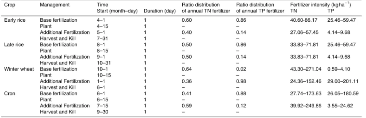
The Shaying River Catchment was divided into 46 subbasins. According to the landuse classification standard of China (CNS, 2007), the main land use types were dry land
15
(84.04 %), forest (7.66 %), urban (3.27 %), grassland (2.68 %), water (1.43 %), paddy (0.91 %) and unused land (0.01 %). The soil input parameters (the contents of sand, clay and organic matter) were calculated based on the percentage of soil types in each subbasin. The main crops were the early rice and late rice in the paddy land, and the winter wheat and corn in the dry land. Their main agricultural management
20
schemes (fertilization, plant, harvest and kill) were summarized by field investigation referred to Wang et al., (2008) and Zhai et al. (2014) (Table 2). The crop rotation and their management schemes were considered in the model by setting the start time and duration of management and the fertilizer amounts used. Only two fertilizations (base and additional fertilization) were designed in the model during the complete growth
25
HESSD
12, 4997–5053, 2015Integrated water system simulation
Y. Y. Zhang et al.
Title Page
Abstract Introduction
Conclusions References
Tables Figures
◭ ◮
◭ ◮
Back Close
Full Screen / Esc
Printer-friendly Version Interactive Discussion
Discussion
P
a
per
|
Discussion
P
a
per
|
Discussion
P
a
per
|
Discussion
P
a
per
|
The daily data series at 65 precipitation stations and six temperature stations were interpolated to each subbasin from 2003 to 2008, using the inverse distance weight-ing method and the nearest-neighbor interpolation method, respectively. The social and economic data (e.g., population and livestock in the rural area, chemical fertilizer amount) were calculated for each subbasin based on the area percentage.
5
Moreover, 23 major dams and sluices and more than 200 urban wastewater dis-charge outlets were considered in the model according to the geographical positions. The farm manure from rural living and livestock farming were considered in the model as nonpoint source due to the scattered characteristics and the deficiency sewage treatment facilities in the rural area.
10
2.3.3 Model evaluation
NH4-N concentration is one of the widely used indices to assess water quality condition
in China (CSEPA, 2002). Thus, both the observation series of daily runoffand NH4-N
concentration were used to calibrate the model parameters. There were five regulated stations (Luohe, Zhoukou, Huaidian, Fuyang and Yingshang) and one unregulated
sta-15
tion (Shenqiu) (e.g., the upstream stations unaffected by water projects, or downstream stations situated far from water projects).
We selected LH-OAT for parameter sensitivity analysis and SCE-UA for parameter calibration in the PAT. The initial parameter values were preset randomly from the value ranges determined by their physical characteristics. The evaluation indices used are
20
bias,r and NS as a demonstration of the extended model. However, NS is sensitive to
extreme value, outlier and number of data points and is not commonly applied in the environmental sciences (Ritter and Muñoz-Carpena, 2013). Thus NS was not used to
evaluate the NH4-N concentration simulation. Furthermore, as the real observed yields
of nonpoint pollutant loads and crops were hard to collect for the whole catchment
25
HESSD
12, 4997–5053, 2015Integrated water system simulation
Y. Y. Zhang et al.
Title Page
Abstract Introduction
Conclusions References
Tables Figures
◭ ◮
◭ ◮
Back Close
Full Screen / Esc
Printer-friendly Version Interactive Discussion
Discussion
P
a
per
|
Discussion
P
a
per
|
Discussion
P
a
per
|
Discussion
P
a
per
|
The model calibration was conducted step-by-step as follows. Hydrological param-eters were calibrated first against the observed runoffseries at each station from
up-stream to downup-stream, and then water quality parameters against the observed NH4-N
concentration series. The calibration and validation periods were from 2003 to 2005 and from 2006 to 2008, respectively. To reduce the dimensions of the calibration
prob-5
lem, we restricted SCE-UA to calibrate only the sensitive parameters as defined by
LH-OAT. Weighting method was usually used to comprehensively handle different
ob-jectives (Efstratiadis and Koutsoyiannis, 2010). In this study, these objective functions were simply aggregated to single objectives (frunoffandfNH4-N) as
frunoff=min[(|bias|+2−r−NS)/3]
fNH4-N=min[(|bias|+1−r)/2]
(1)
10
because the case study was only a demonstration of the model performance.
Moreover, because of the high regulation in most rivers, it is necessary to consider the impact of dam regulation in the integrated water system models. The dam and sluice regulation usually disturbs the intra-annual distribution of flow events, e.g., flat-tening high flow and increasing low flow. The simulation performances of high and low
15
flow were evaluated separately, and the effectiveness of the DRM was tested by
com-paring the simulation with and without considering the regulation. The high and low flow was determined by cumulative distribution function (CDF) and the threshold of 50 % was used for easy presentation, that is, the flow was treated as high flow (or low flow) if its percentile was greater than (or smaller than) the threshold.
20
3 Results and discussion
3.1 Parameter sensitivity analysis
HESSD
12, 4997–5053, 2015Integrated water system simulation
Y. Y. Zhang et al.
Title Page
Abstract Introduction
Conclusions References
Tables Figures
◭ ◮
◭ ◮
Back Close
Full Screen / Esc
Printer-friendly Version Interactive Discussion
Discussion
P
a
per
|
Discussion
P
a
per
|
Discussion
P
a
per
|
Discussion
P
a
per
|
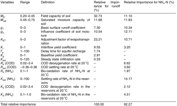
yield coefficient) and Ksat (steady state infiltration rate); TVGM parameters g1 (basic
surface runoff coefficient) and g2 (influence coefficient of soil moisture) for surface
runoff calculation; ground water recharge parameters Kg (baseflow yield coefficient)
andTg(delay time for aquifer recharge); and adjusted factorKETof evapotranspiration.
All these parameters controlled the main hydrological processes, in which soil water
5
and evapotranspiration processes were distinctly important, explaining 54.3 and 23.2 % of the runoffvariation, respectively.
For NH4-N concentration simulation, more than 90 % of observed NH4-N
concentra-tion variaconcentra-tion were explained by 14 sensitive parameters which were categorized into
hydrological (59.28 % of variation), NH4-N (20.65 % of variation) and COD (12.34 % of
10
variation) related parameters. The main explanations were that hydrological processes provided the hydrological boundaries which affected the nonpoint source pollutant load into rivers, the degradation and settlement processes of NH4-N in water bodies (rivers
and reservoirs) (van Griensven et al., 2002). NH4-N concentration was further
influ-enced by the settling and biological oxidation processes. Moreover, it was a
competi-15
tive relationship between COD and NH4-N to consume DO of water bodies in a certain
limited level (Brown and Barnwell, 1987).
3.2 Hydrological simulation
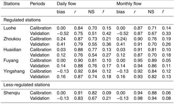
The simulations fitted the observations well at all the stations from the midstream to downstream (Fig. 7 and Table 4). The biases were very close to 0.0 at all the
regu-20
lated stations except Zhoukou with the underestimation (0.24 for calibration and 0.41 for validation) and Luohe with overestimation (−0.52 for validation). The reason of the obvious biases was that the calibration was to obtain the optimal solution for the
av-erage of three evaluation indices, rather than the bias only. Ther values ranged from
0.75 (Luohe for validation) to 0.92 (Yingshang for calibration) with the average value of
25
HESSD
12, 4997–5053, 2015Integrated water system simulation
Y. Y. Zhang et al.
Title Page
Abstract Introduction
Conclusions References
Tables Figures
◭ ◮
◭ ◮
Back Close
Full Screen / Esc
Printer-friendly Version Interactive Discussion
Discussion
P
a
per
|
Discussion
P
a
per
|
Discussion
P
a
per
|
Discussion
P
a
per
|
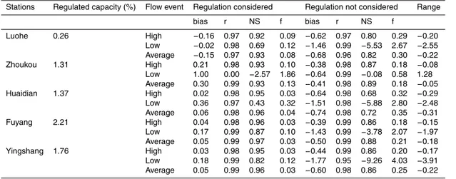
By comparing the simulation results with the observations from 2003 to 2008, we can see that the high and low flows were usually overestimated at all the stations if the model did not consider the regulations (Fig. 8). Except the high flow events at Zhoukou, both high and low flow events at all the stations were simulated better when the dam and sluice regulation was considered (Table 5). The best fitting was at Fuyang,
5
especially for the high flow simulation (bias=0.10, r=0.89 and NS=0.78). From
un-regulation to un-regulation settings, the improvements measured by frunoff ranged from
−0.08 (Zhoukou) to−0.29 (Huaidian) for high flow simulation, from−0.05 (Zhoukou) to −0.31 (Huaidian) for average flow simulation, and from−1.97 (Fuyang) to−3.91 (Ying-shang) for low flow simulation except Zhoukou (1.28). The improvements of simulation
10
performance of low flows were the most obvious. However, their performance still need to be improved further, especially the underestimation at Zhoukou and Huaidian. The
possible reasons were that, on the one hand, the applied evaluation indices (r and NS)
are known to emphasize on the high flows and are disadvantageous to evaluate the low flow simulation (Pushpalatha et al., 2012) and the objective of autocalibration was
15
to obtain the optimal solution for the average of three evaluation indices, rather than the bias only. The slightly sacrifice of bias improved the overall simulation performance evaluated by these three indices. One the other hand, the dam regulation module is still not able to fully capture the low flow events.
In addition, the model performances of monthly flows were even better, particular for
20
rand NS. The values ofr ranged from 0.87 (Luohe for both calibration and validation) to 0.95 (Fuyang for calibration) with the mean of 0.92, while the values of NS ranged from 0.67 (Luohe for validation) to 0.94 (Shenqiu for validation) with the mean of 0.80. Zhang et al. (2013) reproduced the long-term monthly flows by SWAT at the same stations. In comparison with the existing results, the extended model improved the flow simulations
25
HESSD
12, 4997–5053, 2015Integrated water system simulation
Y. Y. Zhang et al.
Title Page
Abstract Introduction
Conclusions References
Tables Figures
◭ ◮
◭ ◮
Back Close
Full Screen / Esc
Printer-friendly Version Interactive Discussion
Discussion
P
a
per
|
Discussion
P
a
per
|
Discussion
P
a
per
|
Discussion
P
a
per
|
3.3 Water quality simulation
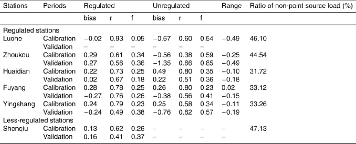
The simulated concentrations matched well with the observations according to the
eval-uation standard recommend by Moriasi et al. (2007) (Fig. 9 and Table 6). Ther values
of all the stations were over 0.60 expect Zhoukou (0.56 for validation), Yingshang (0.49 for validation) and Shenqiu (0.41 for validation) with the average value of 0.67. The bias
5
of all the stations were considered as “acceptable” with the range from−0.27 (Fuyang
for validation) to 0.29 (Zhoukou for calibration). The best simulation was at Luohe. The obvious discrepancies between the simulation and observation often appeared in the period from January to May because of the poor simulation performance of low flows.
The simulation was also significantly improved when the regulation was considered
10
in comparison with the results without the consideration of regulation, except at Fuyang for calibration. The decreases offNH4−Nvalue ranged from 0.10 (Huaidian for
calibra-tion) to 0.49 (Zhoukou for validacalibra-tion) although it was increased slightly at Fuyang for calibration (0.02). The regulation of dams and sluices played a critical role in the water quality simulation. In the upperstream of Shaying River, the flow was small and the
15
pollutant concentration reduced obviously, due to the degradation and settlement of large water storage. In the downstream of Shaying River, the pollutant concentration in-creased due to the pollutant accumulation and the decreasing of flow by the regulation of dams and sluices (Zhang et al., 2010). Therefore, the simulated concentrations with-out regulation were usually overestimated or greater than the simulation with regulation
20
at the upperstream stations (Luohe and Zhoukou), but they were underestimated at the
downstream stations (Huaidian, Fuyang and Yingshang). The largest difference of
sim-ulation between with and without the regsim-ulation consideration appeared at Zhoukou.
The spatial pattern of average annual nonpoint source NH4-N loads was shown
in Fig. 10a. The modeled annual yield rates ranged from 0.048 t km−2year−1 to
25
HESSD
12, 4997–5053, 2015Integrated water system simulation
Y. Y. Zhang et al.
Title Page
Abstract Introduction
Conclusions References
Tables Figures
◭ ◮
◭ ◮
Back Close
Full Screen / Esc
Printer-friendly Version Interactive Discussion
Discussion
P
a
per
|
Discussion
P
a
per
|
Discussion
P
a
per
|
Discussion
P
a
per
|
load of each administrative region which estimated based on the soil erosion, landuse and fertilizer amount in the official report (Wang, 2011), the bias of simulated nonpoint source load in the whole region was 21.31 % when the two regions with great bias (i.e., Fuyang and Pingdingshan) were excluded as the outliers. The high load yield re-gions were in the middle of Pingdingshan, Xuchang, Zhengzhou, Fuyang and Zhoukou
5
regions. The spatial pattern was significantly correlated with the distribution of paddy area (r=0.506, p <0.001) and rice yield (r=0.799, p <0.001) (Fig. 10b and c). The fertilizer loss in the paddy areas might be the primary contributor to the nonpoint source NH4-N load, possibly because the average nitrogen loss coefficient in China was just
30∼70 % in the paddy areas, which was greater than that in the dry areas (20∼50 %)
10
(Zhu, 2000; Xing and Zhu, 2000).
The observed average annual point source NH4-N loads into rivers were about
4.70×10⁴t year−1 in the Shaying River Catchment, which were summarized from the
collected data for model input. The nonpoint source load contributed 18.66 % of the overall NH4-N load on average from 2003 to 2005, which was little less than the
statis-15
tical results (29.37 %) given in the official report (Wang, 2011). Moreover, the contribu-tions of non-point source load at the stacontribu-tions ranged from 31.72 (Huaidian) to 47.13 % (Shenqiu). In comparison with the nonpoint source load of each administrative region in 2000, the simulated annual loads tended to decrease from 2003 to 2005 except in Lu-oyang and Pingdingshan regions. The decrease rate in the entire region was 26.30 %.
20
The primary pollution source in the Shaying River Catchment was still the point source, but the non-point source was also of great concern and its spatial characteristic was that the contribution of nonpoint source was greatest in the upstream, and was lowest in the middle and downstream because the point source load emission was usually concentrated in the this region. Therefore, in comparison with the results of Zhang
25
et al. (2013), the overall simulation performance of NH4-N concentration was also
HESSD
12, 4997–5053, 2015Integrated water system simulation
Y. Y. Zhang et al.
Title Page
Abstract Introduction
Conclusions References
Tables Figures
◭ ◮
◭ ◮
Back Close
Full Screen / Esc
Printer-friendly Version Interactive Discussion
Discussion
P
a
per
|
Discussion
P
a
per
|
Discussion
P
a
per
|
Discussion
P
a
per
|
3.4 Crop yield simulation
The simulated corn yield and its spatial pattern were shown in Fig. 11. The av-erage annual yields were summarized at subbasin scale and ranged from 0.08 to 326.95 t km−2year−1 with the average value of 76.84 t km−2year−1. The yield of each administrative region was further summarized and compared with the data from
statis-5
tical yearbooks from 2003 to 2005 (Henan Statistical Yearbook, 2003, 2004 and 2005) to test the simulation performance (See the inset of Fig. 11). The high-yield regions were Luohe, Fuyang and Zhoukou in the middle and down reaches, whose primary land use were dry land (93.12, 95.87 and 93.18 %, respectively). The yields of Luohe, Nanyang, Kaifeng regions were well simulated. The total yield was underestimated in
10
the whole basin with the bias of 19.93 %. The discrepancies might be caused by the boundary mismatch between the administrative region and subbasin, obvious spatial heterogeneities of human agricultural activities, and the inaccurate cropping patterns in such huge region. Higher resolution remote sensing image and field investigation might improve the model performance.
15
4 Conclusions
In this study, an integrated water system model was developed on the basis of TVGM hydrological model to address water issues emerged in the complex basins and the model performance was demonstrated in the Shaying River Catchment of China by comparing with the observations of several key components of major processes, such
20
as runoff, water quality concentrations, nonpoint source pollutant load and crop yield. The extended model integrates multi-scale processes and their interactions at the field, subbasin scales into a unified system using the two critical and inseparable link-ages, e.g. water and nutrient (N, P and C). The model provides a reasonable tool
for the effective water governance by capturing some indicative components of water
25
HESSD
12, 4997–5053, 2015Integrated water system simulation
Y. Y. Zhang et al.
Title Page
Abstract Introduction
Conclusions References
Tables Figures
◭ ◮
◭ ◮
Back Close
Full Screen / Esc
Printer-friendly Version Interactive Discussion
Discussion
P
a
per
|
Discussion
P
a
per
|
Discussion
P
a
per
|
Discussion
P
a
per
|
water and evaporation, plant transpiration, runoff and water storage in the dams and
sluices), water quality components (e.g., nonpoint source nutrient load, water quality concentrations in water bodies), as well as ecological components (crop yield) which could be calibrated if the observations are available. The case study has shown that the simulated runoffs at most stations fitted the observations well in the highly
regu-5
lated Shaying River Catchment. All the evaluation criteria were acceptable for both the daily and monthly simulations except at one or two stations. This model captured the variation of discontinuous daily NH4-N concentration and properly simulated the spatial
patterns of nonpoint source pollutant load and corn yield.
Due to the heterogeneity of spatial data in large basins and insufficient observations
10
of every subsystems, not all the results were acceptable and several processes were still not well calibrated (low flow events, nonpoint source pollutant load and crop yield, etc.). The model could be improved by further exploring the water related processes. More complex humanity activities and water-related processes in the agricultural man-agement, urban area and economy system will be incorporated into this model once
15
the interaction mechanisms with natural hydrologic cycle could be depicted accurately. Additionally, there are still several great challenges in the combined calibration of
multi-component and model uncertainty analysis because of the interactions and tradeoffs
among different processes. The over-parameterization and the reasonable initial
con-ditions of parameters need also be treated carefully in applications. Advanced
math-20
ematic analysis technologies should be applied in the future works, such as multi-objective optimization algorithm.
Appendix A: Hydrological cycle module
The basic water balance equation is
Pi+SWi =SWi+1+Rsi+Eai+Rssi+Rgi+Ini (A1)
HESSD
12, 4997–5053, 2015Integrated water system simulation
Y. Y. Zhang et al.
Title Page
Abstract Introduction
Conclusions References
Tables Figures
◭ ◮
◭ ◮
Back Close
Full Screen / Esc
Printer-friendly Version Interactive Discussion
Discussion
P
a
per
|
Discussion
P
a
per
|
Discussion
P
a
per
|
Discussion
P
a
per
|
whereP is precipitation (mm); SW is soil water moisture (mm); Ea is actual
evapotran-spiration (mm) including soil evaporation (Es, mm) and plant transpiration (Ep, mm);
Rs, Rss and Rg is surface runoff, interflow and baseflow (mm), respectively; In is the vegetation interception (mm) andi is the time step (day).
Esand Epare determined by potential evapotranspiration (E0, mm), leaf area index
5
(LAI, m2m−2) and surface soil residues (rsd, t ha−1) (Ritchie, 1972) as.
Ea=Et+Es≤E0
Ep=
LAI ·E0/3 0≤LAI ≤3.0
E0 LAI >3.0
Es=E0·exp(−5.0×10− 5
·rsd)
(A2)
whereE0is calculated by Hargreaves method (Hargreaves and Samani, 1982).
The surface runoff(Rs, mm) yield equation (TVGM; Xia et al., 2005) is given as
Rs=g1 SWu/Wsat
g2·(P −In) (A3)
10
where SWuand Wsat are surface soil moisture and saturation moisture (mm),
respec-tively;g1andg2are coefficients of basic runoffand soil moisture, respectively.
The interflow (Rss, mm) and baseflow (Rg, mm) are considered as a linear
storage-outflow relationship (Wang et al., 2009) as
Rss=kr·SWu
Rg=kg·SWl
(A4)
15
wherekr and kgare the yield coefficients of interflow and baseflow, respectively; SWl
is soil moisture of lower layer (mm).
The infiltration from the upper to lower soil layer is calculated using storage routing methodology (Neitsch et al., 2011) as
Winf=(SWu−Wfc)·[1−exp(−t/Tinf)]
Tinf=(Wsat−Wfc)/Ksat
(A5)
HESSD
12, 4997–5053, 2015Integrated water system simulation
Y. Y. Zhang et al.
Title Page
Abstract Introduction
Conclusions References
Tables Figures
◭ ◮
◭ ◮
Back Close
Full Screen / Esc
Printer-friendly Version Interactive Discussion
Discussion
P
a
per
|
Discussion
P
a
per
|
Discussion
P
a
per
|
Discussion
P
a
per
|
whereWinf is water infiltration amount on a given day (mm); Wfc is soil field capacity
(mm);tandTinfare time step and travel time for infiltration (hrs), respectively; andKsat
is saturated hydraulic conductivity (mm h−1).
The calculation of overland flow routing is adopted from Neitsch et al. (2011) as
Qoverl=(Q′overl+Qstor,i−1)·
1−exp(−Tretain/Troute)
Troute=Toverl+Trch=
L0.6overl·n0.6overl
18·slp0.3overl +
0.62·Lrch·n0.75rch
A0.125·slp0.375 rch
(A6)
5
whereQoverlis the overland flow discharged into main channel (mm);Q′overlis the lateral flow amount generated in the subbasin (mm),Qstor,i−1is the lateral flow in the previous
day (mm); Tretain is the retain time of flow (days);Troute, Toverl and Trch are the routing
times of the total flow, overland flow and river flow, respectively (days);Loverland Lrch
are the lengths of subbasin slope and river, respectively (km); slpoverland slprchare the
10
slopes of subbasin and river, respectively (m m−1); noverl and nrch are the Manning’s
roughness coefficients for subbasin and river, respectively (m m−1); Ais the subbasin area (km2).
Appendix B: Soil biochemical module
B1 Soil temperature (Williams et al., 1984)
15
T(Z,t)=T+(AM/2·cos[2π·(t−200)/365]+TG−T(0,t))·exp(−Z/DD) (B1)
whereZis soil depth (mm);tis time step (days);T and TG are average annual