www.ccarevista.ufc.br ISSN 1806-6690
Use of capacitive sensors with the instantaneous profile method to
determine hydraulic conductivity
1Utilização de sensores capacitivos no método do perfil instantâneo para obtenção da
condutividade hidráulica
Eurileny Lucas de Almeida2*, Adunias dos Santos Teixeira3, Odílio Coimbra da Rocha Neto3, Raimundo Alípio
de Oliveira Leão3 and Francisco José Firmino Canafístula3
ABSTRACT - Due to the need to monitor soil water tension continuously, the instantaneous profile method is considered laborious, requiring a lot of time, and especially manpower, to set up and maintain. The aim of this work was to evaluate the possibility of using capacitive sensors in place of tensiometers with the instantaneous profile method in an area of the Lower Acaraú Irrigated Perimeter. The experiment was carried out in a Eutrophic Red-Yellow Argisol. The sensors were installed 15, 30, 45 and 60 cm from the surface, and powered by photovoltaic panels, using a power manager to charge the battery and to supply power at night. Records from the capacitive sensors were collected every five minutes and stored on a data acquisition board. With the simultaneous measurement of soil moisture obtained by the sensors, and the total soil water potential from the soil water retention curve, it was possible to determine the hydraulic conductivity as a function of the volumetric water content for each period using the Richards equation. At the end of the experiment, the advantage of using capacitive sensors with the instantaneous profile method was confirmed as an alternative to using a tensiometer. The main advantages of using capacitive sensors were to make the method less laborious and to allow moisture readings at higher tensions in soils of a sandy texture.
Key words: Richards equation. Unsaturated water flow. Soil dielectric constant.
RESUMO - Devido à necessidade de monitoramento da tensão da água no solo de forma contínua, o método do perfil instantâneo é considerado trabalhoso, sendo necessário muito tempo e, principalmente, mão de obra na instalação e manutenção. O objetivo deste trabalho é avaliar a possibilidade de utilização de sensores capacitivos no método do perfil instantâneo em substituição aos tensiômetro em uma área do Perímetro Irrigado Baixo Acaraú. O experimento foi realizado em um ARGISSOLO VERMELHO-AMARELO Eutrófico. Os sensores foram instalados a 15; 30; 45 e 60 cm da superfície e alimentados por painéis fotovoltaicos, com gerenciador de energia para carregamento de baterias e fornecimento noturno de energia. Os registros dos sensores capacitivos foram coletados a cada cinco minutos e armazenados em placa de aquisição de dados. Dispondo-se das medidas simultâneas de umidade do solo obtidas pelos sensores, e do potencial total da água no solo, pela curva de retenção de água no solo, foi possível a determinação, para cada período, da condutividade hidráulica em função do conteúdo volumétrico de água, através da equação de Richards. Ao final do experimento pode-se concluir pela vantagem da utilização dos sensores capacitivos no método do perfil instantâneo como alternativa ao uso do tensiômetro. As principais vantagens do uso de sensores capacitivos foi a de tornar o método menos trabalhoso e possibilitar a leitura da umidade em maiores tensões nos solos de textura arenosa.
Palavras-chave: Equação de Richards. Fluxo não saturado de água. Constante dielétrica do solo.
DOI: 10.5935/1806-6690.20180040 *Author for correspondence
Received for publication 02/10/2015; approved on 29/06/2017
1Parte da Dissertação do primeiro autor, apresentado ao Programa de Pós-Graduação em Ciência do Solo da Universidade Federal do Ceará
2Departamento de Ciência do Solo, Universidade Federal do Ceará/UFC, Av. Mister Hull, 2977, Campus do Pici, Bloco 807, Fortaleza-CE, Brasil,
60.440-554, [email protected]
3Departamento de Engenharia Agrícola, Universidade Federal do Ceará/UFC, Av. Mister Hull, 2977, Campus do Pici, Bloco 804, Fortaleza-CE, Brasil,
INTRODUCTION
The availability and movement of water in the soil are important factors for crop growth and productivity, since as well as satisfying water demand they determine plant access to nutrients. As the soil is the main water reservoir for plants, it becomes essential to determine its hydraulic properties.
Among the hydraulic properties of the soil, hydraulic conductivity is important as it reflects the ease with which water moves in a saturated or unsaturated profile. Study of the unsaturated state is particularly significant due to the occurrence of processes intrinsic to irrigation management, such as infiltration, drainage (LIBARDI; MELO FILHO, 2006) and absorption by plants.
The relationship that best describes soil water flow is the Darcy-Buckingham equation (Equation 1) in which the hydraulic conductivity (K) is the proportionality constant between the flow density (q) and the total water potential gradient (∆Ψt/L).
q = -K(Ө) ∆Ψt/L (1)
where: ө - soil moisture.
In addition to total water potential Ѱt, the hydraulic conductivity also determines flow behaviour (AMARO FILHO; ASSIS JUNIOR; MOTA, 2008; GONÇALVES; LIBARDI, 2013). According to Equation 1, the higher the hydraulic conductivity, the greater the ease with which water moves in the soil, reaching maximum value with saturation. However, high hydraulic conductivity does not necessarily imply a greater flow, since the flow is also dependent on the potential gradient (REICHARDT, 1990). Movement occurs to decrease this potential, i.e. the water moves from points of greater potential towards the points of least potential.
Several methods are presented in the literature for measuring hydraulic conductivity, being divided into field and laboratory methods (GHIBERTO; MORAES, 2011). Under field conditions, the most commonly used is the instantaneous profile method, with the advantage of being a direct field measurement, resulting in more-accurate values for hydraulic conductivity when compared with laboratory methods (GONÇALVES; LIBARDI, 2013).
Since the instantaneous profile method is considered laborious, requiring a lot of time and manpower to set up and maintain, it is assumed that alternatives which are able to reduce the disadvantages of the method are necessary and will be very attractive. The use of transducers (electronic sensors) to replace the tensiometers used with the instantaneous profile is very
promising, mainly due to speed and automation making it easier to monitor the soil water content.
The operating principle of capacitive sensors is based on electrical capacitance. As this is non-destructive, application of these sensors has been studied in research relating to soil moisture (CRUZ et al., 2010; FREITAS et al., 2012, LEÃO et al., 2007), where their ability to provide the soil water content at any depth with a relatively high level of accuracy has been verified. This is possible because the technique of electrical capacitance is a method capable of measuring dielectric permittivity in the soil, and can be used frequently to measure the water content. (GARDNER; DEAN; COOPER, 1998; TEIXEIRA; COELHO, 2005).
With the intention of proposing a more accurate and less laborious alternative for recording soil moisture, this study proposes the use of capacitive sensors to replace tensiometers in the instantaneous profile field method, in a soil of the Lower Acaraú Irrigated Perimeter.
MATERIAL AND METHODS
Calibration of the capacitive sensors in the field
The capacitive sensors, the data acquisition system, and the power manager used in the experiment were developed at the Agricultural Electronics and Mechanics Laboratory (LEMA) of the Department of Agricultural Engineering (DENA), at the Federal University of Ceará (UFC). These sensors have already been used in several studies (CRUZet al., 2010; ROCHA NETOet al., 2005; TEIXEIRA; COELHO, 2005), and have proved efficient in the real-time automatic monitoring of soil moisture.
The sensors (Figure 1) are based on Frequency-Domain Reflectance (FDR), which also relates soil capacitance to moisture.
In calculating the capacitance (Equation 2) applied to the sensors being used, only the dielectric constant of the medium is variable, since the area of the plates and the distance between them are fixed and determined at the time the sensor is constructed. Therefore, the charge and discharge frequency of the capacitor depends directly on the material between the plates. Once installed in the soil, the greatest variation in the dielectric constant will be caused by the passage or accumulation of water in the region, relating the frequency to the water content of the soil.
Cαεrε0A/d (2)
where:C - capacitance,A - area of the plates,d - distance between plates, εr- dielectric constant of the medium, and
Figure 1 - Capacitive soil moisture sensor
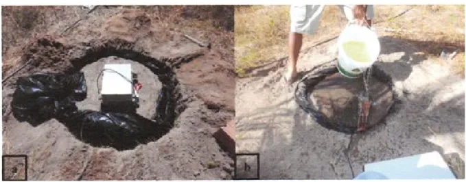
To calibrate the capacitive sensors in the field, an area, 60 cm in diameter by 30 cm in depth, was marked out in a plot in the Lower Acaraú Irrigated Perimeter, where the soil is a Eutrophic Red-Yellow Argissol with an average sand, silt and clay content of 814.38, 57.41 and 128.21 g kg-1 respectively. The sides of the area were coated with plastic, allowing free drainage only along the vertical (Figure 2a). Soil saturation began after a capacitive sensor had been installed in the centre of the area (Figure 2b).
The soil was considered saturated when the data recorded by the capacitive sensor stabilised. After saturation, soil samples were collected as the water was drained and/or evaporated, and at the same time, recorded data were obtained with the capacitive sensor. The containers with the wet soil samples were then weighed on a tenth-gram precision scale and placed in an oven at 105°C for 24 hours to obtain the mass-based moisture by the gravimetric method. Three soil samples were collected using an Uhland sampler to obtain total bulk density, required to determine the moisture content on a volumetric basis. Equations 3, 4 and 5 represent the process to determine volumetric moisture.
Figure 2 - Calibration of the sensor in the field: a – marking out the area to be used; b - saturation of the area ρs= m
s/Vs (3)
u = (mu - ms)/ms (4)
Ө = ρs. u (5)
where:ρs - total soil bulk density (kg m
-3);m
s - dry soil
weight (kg);mu - moist soil weight (kg);Vs - soil volume (m³);u - mass-based soil moisture (kg.kg-1); Ө - volumetric moisture (m3 m-3).
After field calibration, the frequency records obtained with the capacitive sensors, and the volumetric humidity were analysed using the IBM SPSS Statistics software to obtain the calibration equation. The following models were tested: linear, quadratic, exponential, logarithmic and potential. Finally, the curve with the greatest coefficient of determination and the smallest standard error of the estimate was chosen.
Instantaneous Profile
To use the Instantaneous Profile method, an experimental plot with a diameter of 3.0 m was marked out, which was delimited laterally with plastic sheeting and surrounded by ridges approximately 0.3 m in height to contain the water to be applied in saturating the soil (Figure 3).
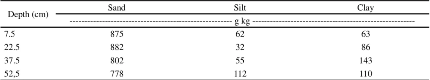
Two batteries of sensors were used, installed in the centre of the area 1.3 m apart, each composed of four capacitive moisture sensors. The sensors were spaced 50 cm apart, at depths of 0.075, 0.225, 0.375 and 0.525 m, representing the 0-0.15 m, 0.15-0.30 m, 0.30-0.45 m and 0.45-0.60 m layer respectively; the granulometry can be found in Table 1.
profile at the depth of 0.6 m, soil saturation being verified by the proximity of the values recorded by the sensors. After the soil was saturated, the area was covered with polyethylene sheeting to avoid loss by evaporation or the entry of water through the surface; finally, a layer of straw was placed over the area to avoid large fluctuations in soil temperature (Figure 4a).
With the start of drainage, data recorded with the capacitive sensors were collected every 5 minutes and stored in the memory of the Data Acquisition System - DAS. During the daytime, the sensors were powered by the photovoltaic panels, and at night by battery, charged during the day by the same panels by means of a photovoltaic battery charge manager (Figures 4a and 4b). At the end of each day, the data were collected and the memory of the DAS was cleared. This process continued for 30 days.
Moisture values were calculated from the data provided by the capacitive sensors using the calibration equation carried out in the field. The values for matrix potential (Ѱm) were determined as a function of the moisture submitted to the soil water
Figure 3 - Marking out the experimental plot for the instantaneous profile test
Table 1 - Representative sand, silt and clay content at the four depths in the study area
Source: Caitano, 2009
retention curve obtained by the Whatman No 42 Filter Paper method, a method widely used in the literature (BEDDOE; TAKE; ROWE, 2010; BULUT; LEONG,
2008; LUCAS et al., 2011). The value of the matrix
potential was therefore obtained indirectly by means of the capacitive sensors.
The total potential (Ѱt) was calculated
considering the soil surface as gravitational reference, and being equal to the sum of the gravitational potential (Ѱg) and matrix potential (Ѱm); Ѱg was considered as 15 cm, 30 cm, 45 cm and 60 cm at the respective depths.
From the simultaneous measurement of the moisture and the total soil water potential throughout the profile, the hydraulic conductivity (K) was determined for each time period as a function of the volumetric water content (θ) by the Richards equation (Equation 6), a combination of the Darcy-Buckinhgam Equation (Equation 1) and the continuity equation, which gives the general differential governing the movement of water in the soil (GONÇALVES; LIBARDI, 2013; WENDLAND; PIZARRO, 2010).
Depth (cm) Sand Silt Clay
g kg
---7.5 875 62 63
22.5 882 32 86
37.5 802 55 143
Figure 4 - a. Experimental area covered with plastic and straw, b. equipment for acquisition of the capacitive sensor data
(6)
where the numerator is the flow density and the denominator is the total potential gradient at soil depth Z.
RESULTS AND DISCUSSION
Calibration of the capacitive sensor
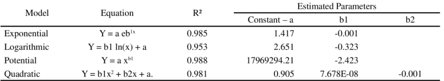
The relationship between soil moisture and the frequency responses of the capacitive sensor installed in the field can be seen in Figure 5. The hypothesis that regression is significant at a level of 99.9% was validated by F-test, carried out using the IBM SPSS Statistics software.
The model that best fit the data was the potential, whose coefficient of determination demonstrated the highest correlation of moisture data with sensor frequency. The exponential equation overestimated moisture values by 10 to 20%. The coefficient of determination (R2) and
estimated parameters for four of the models under study are shown in Table 2.
Instantaneous Profile Method for determining the value of K(θ)
Figure 6 shows the behaviour of the sensor registers (kHz) with time (h) at depths of 15, 30, 45 and 60 cm. Initially, the sensor data are similar, continuing almost in parallel up to around 200 hours. From 450 hours, the
Figure 5 - Volumetric humidity as a function of frequency in
the field calibration
Model Equation R² Estimated Parameters
Constant – a b1 b2
Exponential Y = a eb1x 0.985 1.417 -0.001
Logarithmic Y = b1 ln(x) + a 0.953 2.651 -0.323
Potential Y = a xb1 0.988 17969294.21 -2.423
Quadratic Y = b1x2 + b2x + a. 0.981 0.905 7.678E-08 -0.001
sensors installed at depths of 45 and 60 cm recorded similar values, and from this time demonstrated the slower drying of these layers in relation to the other layers, which was due to the higher clay content at depth resulting in greater water retention in these layers and faster drying in the upper layers.
The quickly rising behaviour of the values recorded during the first hour with the capacitive sensor placed at a depth of 15 cm, can be explained by the greater sand content on the surface, justifying faster water loss through leaching.
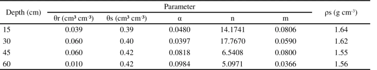
The values of θ were calculated by means of the calibration equation obtained under field conditions. The values for matrix potential were calculated from the parameters of the soil water retention curve (Table 3), obtained by the filter paper method and fitted as per van Genuchten (1980).
The values found for the saturated moisture content, which varied with the increasing depth from 0.39 to 0.42 cm³ cm-3, are consistent with the increase in clay content, since from the textural point of view, the sandier the texture, the lower the water content for a given potential. This is due to the nature of the colloidal
material, mainly a result of the smaller surface area per unit of mass or volume compared to finer material (AMARO FILHO; ASSIS JUNIOR; MOTA, 2008).
Figure 7 shows the potential adjustment for the relationship between moisture and time, with high coefficients of determination for the depths of 30, 45 and 60 cm, while at the depth of 15 cm the coefficient of determination was slightly lower. This can be explained by the greater sand content at the surface, leading to an increase in the number of macropores and to non-uniform pore distribution.
Depth (cm) Parameter ρs (g cm-3)
θr (cm³ cm-³) θs (cm³ cm-³) α n m
15 0.039 0.39 0.0480 14.1741 0.0806 1.64
30 0.060 0.40 0.0397 17.7670 0.0590 1.62
45 0.060 0.42 0.0818 6.5408 0.0800 1.55
60 0.010 0.42 0.0984 5.0971 0.0366 1.56
Table 3 - Parameters of the van Genuchten equation (1980), for four depths
θr and θs - residual and saturated volumetric moisture content respectively; α, m and n - curve parameters; ρs - bulk density
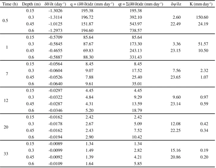
The calculated values for water flow density (q) can be seen in Table 4 for each layer at 12 different distribution times, with dz equal to 15 cm, and the variation in volumetric moisture for the variation in time (δθ/δt) and the hydraulic conductivity at a depth of 30 cm and 45 cm, as per the Richards equation (Equation 2). It can be seen from Table 4 that up to 150 hours the water flow decreased from the first to the third layer, probably due to the reduction in bulk density, as shown in Table 3, and a significant increase in the soil clay content around the third layer (Table 1).
Figure 7 - Volumetric moisture adjustment curves as a function of the soil water redistribution time
From the values of the matrix potential, calculated using the parameters of the characteristic curve fitted by the van Genuchten model (1980), the graphical behaviour of the matrix potential as a function of time (t) was evaluated for the four depths; the equations adjusted by the potential model with their respective coefficients of determination are Ψm = 72.772t0.3119 (R² = 0.94869),
Ψm = 87.048t0.4485 (R² = 0.9274), Ψm = 143.59t0.428 (R² = 0.97820) and Ψm = 751.66t0.855 (R² = 0.9908) for the depths of 15, 30, 45 and 60 cm respectively.
The values ofΨt were calculated considering the soil surface as the gravitational reference, adjusted as a function of depth for the twelve redistribution times evaluated in this study. The total potential gradients as a function of distancez are the result of derivation of the curve fitting equations forΨt againstz, wherez represents a range of depths between an upper and a lower limit, these limits being the installation depths of the sensors
Table 4 - Density values for total flow (q), total potential gradient (δψ/δz) and hydraulic conductivity (K) for depths of 15 to 45 cm and 30 to 60 cm
Time (h) Depth (m) δθ/δt (day-1) q = (δθ/δt)dz (mm day-1) qt = Σ(δθ/δt)dz (mm day-1) δψ/δz K (mm day-1)
0.5
0.15 -1.3026 195.38 195.38
0.3 -1.3114 196.72 392.10 2.60 150.60
0.45 -1.0125 151.87 543.97 22.49 24.19
0.6 -1.2973 194.60 738.57
1
0.15 -0.5709 85.64 85.64
0.3 -0.5845 87.67 173.30 3.36 51.57
0.45 -0.4655 69.83 243.13 23.15 10.50
0.6 -0.5887 88.30 331.43
7
0.15 -0.0564 8.45 8.45
0.3 -0.0604 9.07 17.52 7.56 2.32
0.45 -0.0526 7.88 25.40 23.65 1.07
0.6 -0.0640 9.61 35.01
12
0.15 -0.0297 4.45 4.45
0.3 -0.0322 4.84 9.29 9.60 0.97
0.45 -0.0287 4.31 13.59 23.14 0.59
0.6 -0.0346 5.20 18.79
20
0.15 -0.0162 2.42 2.42
0.3 -0.0178 2.67 5.09 12.08 0.42
0.45 -0.0162 2.43 7.52 22.25 0.34
0.6 -0.0194 2.90 10.42
33
0.15 -0.0089 1.34 1.34
0.3 -0.0099 1.49 2.82 15.16 0.19
0.45 -0.0092 1.39 4.21 20.86 0.20
0.6 -0.0109 1.64 5.85
immediately above and below z. For this reason, total potential gradient and hydraulic conductivity were calculated for the depths of 30 and 45 cm only.
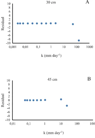
The values for hydraulic conductivity K were determined with the Darcy-Buckingham equation (Table 4). The graph of the K(θ) function and the regression analysis for the depths of 30 and 45 cm can be seen in Figure 8.
45 cm, the adjustment model was the exponential, with a coefficient of determination of 0.998 and standard error of the estimate of 0.083 (Table 5).
It can be seen from Figure 8 that there is a tendency for the hydraulic conductivity of the soil to decrease with depth, which can be explained by the increase in clay content with depth, 9.6% and 15.16% for the depths of 30 and 45 cm respectively. In the Giacheti (2000) experiment in sandy soils, it was found that hydraulic conductivity determined in the laboratory decreases with depth due to a reduction in the number of pores in these soils.
From an analysis of Figure 8 and Table 5 it can be seen that the use of capacitive sensors with
Depth Model R² Standard error of theestimate ANOVA significanceof regression Estimated Parameters
Constant a b1 b2
30 cm
Linear 0.691 25.969 0.001 -74.708 1038.258
Exponential 0.970 0.646 0.000 3.287E-05 98.504
Logarithmic 0.554 31.193 0.006 242.556 90.518
Potential 0.999 0.029 0.000 6.801E+09 9.738
Quadratic 0.937 12.347 0.000 119.134 19545.523 -3138.896
45 cm
Linear 0.786 4.079 0.001 -25.067 244.282
Exponential 0.998 0.083 0.000 0.0001 70.246
Logarithmic 0.711 4.740 0.004 67.488 29.469
Potential 0.994 0.169 0.000 1.15E+08 8.891
Quadratic 0.968 1.712 0.000 56.811 5022.404 -1074.480
Table 5 - Coefficient of determination, standard error of the estimate, significance of regression, and parameters of the models for the
hydraulic conductivity function
Continued Table 4
55
0.15 -0.0048 0.73 0.73
0.3 -0.0055 0.82 1.55 19.13 0.08
0.45 -0.0052 0.78 2.33 18.79 0.12
0.6 -0.0061 0.92 3.24
90
0.15 -0.0027 0.40 0.40
0.3 -0.0031 0.46 0.87 23.97 0.04
0.45 -0.0030 0.45 1.32 15.98 0.08
0.6 -0.0035 0.52 1.84
150
0.15 -0.0015 0.22 0.22
0.3 -0.0017 0.25 0.47 30.29 0.02
0.45 -0.0017 0.25 0.73 12.00 0.06
0.6 -0.0019 0.29 1.02
Figure 9 - Graphical analysis of the residuals: A - potential model and B - exponential model at depths of 30 and 45 cm the instantaneous profile method proved to be quite satisfactory, where the coefficients of determination showed values greater than 0.99, and the standard error of the estimate for the models of hydraulic conductivity against moisture were close to zero at the depths of 30 and 45 cm.
A graphical analysis of the residuals of the potential (A) and exponential (B) models for the depths of 30 and 45 cm respectively can be seen in Figure 9. The residuals are very close to zero, demonstrating that the models were adequate for the data, except for the high values of hydraulic conductivity, where the models underestimated the hydraulic conductivity at both depths.
The instantaneous profile method has become less laborious with the use of capacitive sensors, especially as it is not necessary to collect data manually several times a day since the memory of the data acquisition system can handle 30 consecutive days of data collection without the need for intervention.
CONCLUSION
1. The models that best fit the hydraulic conductivity function were the potential and exponential for a depth of 30 and 45 cm respectively, producing the lowest estimation errors and consequently, residuals close to zero;
2. The main advantage seen with the use of capacitive sensors in the instantaneous profile method was greater efficiency in obtaining the data, since delays at the collection point were reduced with the storage possibilities of the DAS, and the amount of data increased considering the higher frequency of automatic data acquisition and the greater range of soil water potential for which the capacitive sensors can be used. In the final analysis, this efficiency means that the use of capacitive sensors makes the method less laborious; 3. Finally, it is concluded that the capacitive sensor is
an accurate and viable alternative for obtaining soil moisture readings, and is able to replace tensiometers in the instantaneous profile method.
REFERENCES
AMARO FILHO, J.; ASSIS JUNIOR, R. N.; MOTA, J. C. A.
Física do solo: conceitos e aplicações. Fortaleza: Imprensa
Universitária, 2008. 289 p.
BEDDOE, R. A.; TAKE, W. A.; ROWE, R. K. Development of suction measurement techniques to quantify the water retention behaviour of GCLs.Geosynthetics International, v. 17, p. 301-12, 2010.
BULUT, R.; LEONG, E. C. Indirect measurement of suction.
Geotechnical and Geological Engineering, v. 26, p. 633-44, 2008.
CAITANO, R. F. Comparação entre metodologias de determinação da função condutividade hidráulica não saturada. 2009. 79 f. Monografia (Graduação em Agronomia) - Universidade Federal do Ceara, Fortaleza, 2009.
CRUZ, T. M. L. et al.Avaliação de sensor capacitivo para o monitoramento do teor de agua do solo.Engenharia Agrícola,
v. 30, n. 1, p. 33-45, 2010.
FREITAS, W. A.et al. Manejo da irrigação utilizando sensor da umidade do solo alternativo.Revista Brasileira de Engenharia Agrícola e Ambiental, v. 16, n. 3, p. 268-274, 2012.
GARDNER, C. M. K.; DEAN, T. J.; COOPER, J. D. Soil water content measurement with a high-frequency capacitance sensor.Journal of Agricultural Engineering Research, v. 71, n. 4, p. 395-403, 1998.
GHIBERTO, P. J.; MORAES, S. O. Comparação de métodos de determinação da condutividade hidráulica em um latossolo vermelho-amarelo.Revista Brasileira de Ciência do Solo,
GIACHETI, H. L. et al. A condutividade hidráulica de um solo arenoso determinada a partir de ensaios de campo e de laboratório. In: CONGRESSO INTERAMERICANO DE ENGENHARIA SANITÁRIA E AMBIENTAL, 27., 2000, Porto Alegre.Anais...Porto Alegre: Asociación Interamericana de Ingeniería Sanitaria y Ambiental, 2000. CD-ROM. GONÇALVES, A. D. M. A.; LIBARDI, P. L. Análise da determinação da condutividade hidráulica do solo pelo método do perfil instantâneo. Revista Brasileira de Ciência do Solo,
v. 37, p. 1174-1184, 2013.
HILLEL, D. A.; KRENTOS, V. K.; STILIANOV, Y. Procedure and test of an internal drainage method for measuring soil hydraulic characteristics in situ.Soil Science, v. 114, p. 395-400, 1972. LEÃO, R. A. O.. et al. Desenvolvimento de um dispositivo eletrônico para calibração de sensores de umidade do solo.
Engenharia Agrícola, v. 27, n. 1, p. 294-303, 2007.
LIBARDI, P. L.; MELO FILHO, J. F. Análise exploratória e variabilidade dos parâmetros da equação da condutividade hidráulica, em um experimento de perfil instantâneo. Revista Brasileira Ciência do Solo, v. 30, p.197-206, 2006.
LUCAS J. F. R.et al. Curva de retenção de água no solo pelo método do papel-filtro.Revista Brasileira de Ciência do Solo, v. 35, p. 1957-1973, 2011.
REICHARDT, K. A água em sistemas agrícolas. 2. ed. São Paulo: Manole, 1990. 188 p.
ROCHA NETO, O. C. et al. Application of artificial neural networks as an alternative to volumetric water balance in drip irrigation management in watermelon crop. Engenharia Agrícola (Online), v. 35, p. 266-279, 2015.
TEIXEIRA, A. S.; COELHO, S. L. Desenvolvimento e calibração de um tensiômetro eletrônico de leitura automática.Engenharia Agrícola, v. 25, n. 2, p. 367-376, 2005.
VAN GENUCHTEN, M. Th. A closed-from equation for predicting the conductivity of unsaturated soils. Soil Science Society of American Journal, v. 44, p. 892-898, 1980. WENDLAND, E.; PIZARRO, M. L. P. Modelagem computacional do fluxo unidimensional de água em meio não saturado do solo.Engenharia Agrícola, v. 30, n. 3, p. 424-434, 2010.