Frozen Concentrated Orange Juice: why Florida´s
producers are so afraid?
Paulo Sérgio Fracalanza* Adriana Nunes Ferreira** Marcos Fava Neves***
Resumo: Este artigo tem por objetivo contribuir para o exame das implicações em termos da alocação de recursos e de bem-estar de uma eventual redução das barreiras tarifárias no mercado dos EUA de suco de laranja concentrado e congelado (FCOJ) importado do Brasil. Depois da introdução, uma segunda seção apresenta uma visão geral das principais características do mercado e do regime de comércio para o suco de laranja, bem como uma avaliação preliminar dos possíveis impactos da liberalização comercial dentro do quadro de acordos comerciais com o NAFTA e com a União Européia. A terceira seção descreve os modelos de equilíbrio parcial com bens substitutos utilizados para o exame dos impactos em termos de quantidades, preços e bem-estar da redução tarifária nos mercados de FCOJ dos EUA. A quarta seção apresenta dois possíveis cenários da liberalização comercial usando o modelo de «país grande». A última seção sumariza os principais resultados.
Palavras-chave: Liberalização comercial, redução de barreiras tarifárias, modelos de equilíbrio parcial, suco de laranja concentrado e congelado.
*Professor Doutor no Instituto de Economia da Unicamp e nas Faculdades de Campinas (FACAMP). Pesquisador do Núcleo de Economia Industrial e da Tecnologia (NEIT) do IE/Unicamp. [email protected]
**Professora Doutora no Instituto de Economia da Unicamp e Pesquisadora do Núcleo de Economia Industrial e da Tecnologia (NEIT) do IE/Unicamp.
Classificação JEL: F13
Abstract: This study aims at examining the resource allocation and welfare implications of the reduction of barriers in the United States market for Frozen Concentrated Orange Juice (FCOJ) imported from Brazil. The present paper is organized as follows: section 2 presents an overview of the main features of the market and current trade regime for orange juice, as well as the possible impacts of liberalization within FTAA and with the European Union; section 3 describes the partial equilibrium model of imperfect substitute goods used to estimate the impact of trade liberalization in the United States, on prices and quantities and on welfare; in section 4 two possible scenarios for liberalization are designed using the large country model. The last section summarizes the main conclusions.
Key words: Commercial liberalization, reduction of trade barriers, partial equilibrium models, frozen concentrated orange juice (FCOJ).
JEL Classification: F13 - Commercial Policy; Protection; Promotion; Trade Negotiations
1. Introduction
Together, Brazil and the USA comprise over 90% of world output of orange juice. Both countries are large producers, but the Brazilians have reached levels of production costs that the US producers cannot match. Currently, Brazilian exports face high barriers in the USA, and this has led Brazil to lodge complaints at the WTO.
The combination of large efficiency gaps between producers and high barriers make the orange juice industry one of the loci of strong resistance to trade liberalization either in a MERCOSUR-NAFTA agreement or in FTAA.
relatively small and where trade is already intense will probably resist liberalization less than other sectors. Sectors where competitive gaps are large and where trade barriers are currently high are natural candidates to show strong resistance. The sectoral perspective is therefore essential in order to identify potential business support for and/or resistance to further progress in current trade negotiations.
Thus, this study aims at examining the resource allocation and welfare implications of the lowering of barriers in the United States market for frozen concentrated orange juice (FCOJ) imported from MERCOSUR, specifically from Brazil.
The article is organized as follows: section 2 presents an overview of the main features of the market and current trade regime for orange juice, as well as the possible impacts of liberalization within FTAA and with the European Union; section 3 describes the partial equilibrium model of imperfect substitute goods used to estimate the impact of trade liberalization on domestic production in the United States, on prices and quantities and on welfare; in section 4 two possible scenarios for liberalization are designed using the version of a large country model. The last section summarizes the main conclusions.
2. Trade flows and trade policy
2.1. Supply and demand in the international market of FCOJ
The world market for fruit juice is very dynamic. Sales, which showed an average annual growth rate of 5%, reached $31 billion in 1998. Approximately half of that amount results from sales of orange juice.
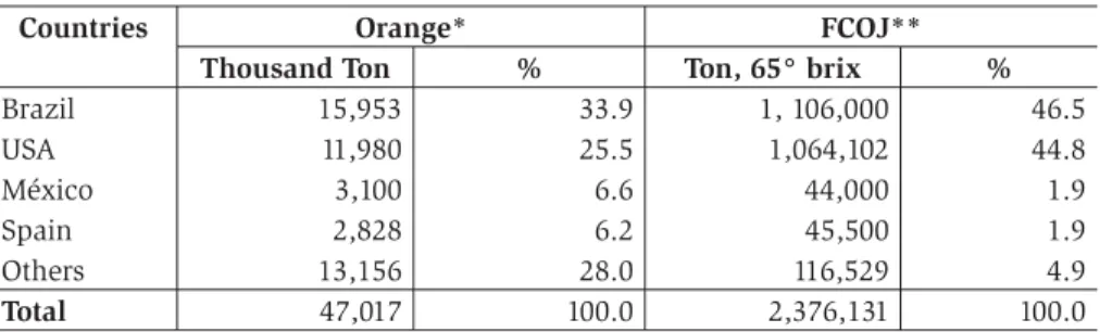
World orange production is concentrated in four countries. Brazil is the major producer with about 27 thousand rural production units, and is responsible for 34% of world orange production and 47% of the total orange juice production. The USA is the second largest producer. Table 1 shows data on the principal producers of oranges and Frozen Concentrated Orange Juice in 1999/2000.
in Brazil has grown 30% over the last decade, reaching 599 boxes per hectare in 2002, well above levels achieved in several countries.
Table 1 – Oranges and FCOJ main producers
Countries Orange* FCOJ**
Thousand Ton % Ton, 65° brix %
Brazil 15,953 33.9 1, 106,000 46.5
USA 11,980 25.5 1,064,102 44.8
México 3,100 6.6 44,000 1.9
Spain 2,828 6.2 45,500 1.9
Others 13,156 28.0 116,529 4.9
Total 47,017 100.0 2,376,131 100.0
Sources: *USDA – United States Department of Agriculture – World Horticultural trade & USA Export Opportunities – February 2001.
** National Agricultural Statistic Service and USA Department of Commerce, Bureau of Census. Florida Department of Citrus. Reports from USA Agricultural counselors and Attachés and/or USDA/FAS Estimates.
However, it is important to point out that average farm productivity in Brazil is lower than in the USA. In Brazil, the yield is around 2 boxes (40.8kg)/tree, while in the USA it is around 3.5 boxes/tree. There are two main reasons for this: firstly, the area used in the USA is almost 100% irrigated, which means increased land productivity; and secondly, the USA produces more Hamlin fruit than Brazil (53% of the USA area, against 13% in Brazil), this being a kind of orange that permits greater volume of juice production, although the quality of the juice is inferior. There are no significant differences in productivity between the Brazilian and US orange juice industries because the equipment used is the same.
Hence, the lower Brazilian production costs are not due to a higher productivity. The main reasons for the superior competitiveness of Brazilian orange juice production are smaller farm inputs, and lower land and labor (used for picking the oranges) costs.
Table 2 – Compared operational costs - Sao Paulo* and Florida**
Operational Costs Sao Paulo Florida
Insecticides 312. 59 51.01
Fungicides 53.83 104.83
Herbicides 12.60 230.73
Fertilizers 214.23 306.62
Operations 333.41 768.27
Irrigation 0.00 372.03
Labor 129.83 178.33
Cost ($/Ha) 1056.48 2011.82
Cost ($/box) 1.27 1.87
Source: Pozzan, M., Muraro, R. and Ueta, F.Z., “Realidades Distintas”, Agroanalysis, revista de Agronegócios da FVG, Agosto 2002. Brazilian data are collected by IEA – Instituto de Economia Agrícola, São Paulo State Department. Florida data were published in Budgeting Costs and Returns for Southeast Florida Citrus Production, 2000-2001, October 2001, UFL publication.
*2001/2002 harvest. ** 2000/2001 harvest
Operational costs are significantly higher in Florida than in Sao Paulo. Brazilian orange production does not utilize irrigation and involves lower labor costs (which also help to explain lower operation costs). In spite of being 90% higher than Sao Paulo’s operational costs when measured per hectare, Florida’s costs differ only 47% from Sao Paulo’s when measured per box. This is explained by the above-mentioned superior productivity per tree of Florida’s production.
Table 3 shows comparative picking and transportation costs for Sao Paulo and Florida orange production. It is clear that these are the main items responsible for the considerably higher orange production costs in Florida. There is a scarcity of local workers for the job and the severe government restrictions on hiring foreign workers raises the cost of labor, so the costs of orange picking and transportation in Florida are even greater than operational costs.
Table 3 – Compared picking and transportation costs – Sao Paulo* and Florida**
Sao Paulo Florida
Picking and loading 333.33 1,635.52
Freightage 125.00 570.28
Cost ($/Ha) 458.33 2,205.80
Source: Pozzan, M., Muraro, R. and Ueta, F.Z., “Realidades Distintas”, Agroanalysis, revista de Agronegócios da FVG, Agosto 2002. Brazilian data are collected by IEA – Instituto de Economia Agrícola, Sao Paulo State Department. Florida data were published in Budgeting Costs and Returns for Southeast Florida Citrus Production, 2000-2001, October 2001, UFL publication.
*2001/2002 harvest. ** 2000/2001 harvest
Finally, table 4 shows the comparison of a third important element in orange production costs in Sao Paulo and Florida: tax payments.
Table 4 – Compared tax payments – Sao Paulo* and Florida**
Tax Payments Sao Paulo Florida
Property tax/Water Management 0.00 145.53
DOC assessment 0.00 175.00
Fundecitrus/Funrural/Senar 75.33 0.00
Total/Hectare ($) 75.33 320.53
Total/Box ($) 0.09 0.30
Source: Pozzan, M., Muraro, R. and Ueta, F.Z., “Realidades Distintas”, Agroanalysis, revista de Agronegócios da FVG, August 2002. Brazilian data are collected by IEA – Instituto de Economia Agrícola, Sao Paulo State Department. Florida data were published in Budgeting Costs and Returns for Southeast Florida Citrus Production, 2000-2001, October 2001, UFL publication.
*2001/2002 harvest. ** 2000/2001 harvest
The most important differences have to do with property, water management and DOC assessment1 taxes; these are not paid by Brazilian
producers but they are a heavy burden in Florida. Brazilian taxes on rural property and to the Citric Producers Association together only add $0.09 per box to the total cost.
In spite of operating with much lower productivity per tree, Brazilian orange producers have huge cost advantages over producers in Florida. The most important factors are operational differences in the cost of picking and transportation, which are mostly due to different prices for labor. This is why, in 2001/2002, with prices per box of $3.54, Florida producers faced a loss of $0.68 per box, while Brazilian producers, with sale prices of $2.75, made a profit of $0.84 per box. Florida producers are investing heavily in picking mechanization in order to reduce that cost disadvantage, but results will not immediately be apparent. 2
1 Tax paid to the Citrus Department for local citric product marketing.
2 The reaction of Florida producers may possibly erode the competitive advantage of
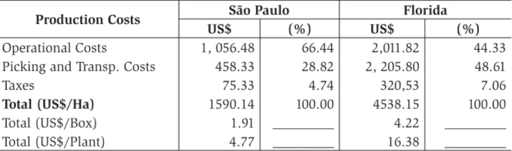
Table 5 – Compared total production costs – Sao Paulo* and Florida**
Production Costs São Paulo Florida
US$ (%) US$ (%)
Operational Costs 1, 056.48 66.44 2,011.82 44.33
Picking and Transp. Costs 458.33 28.82 2, 205.80 48.61
Taxes 75.33 4.74 320,53 7.06
Total (US$/Ha) 1590.14 100.00 4538.15 100.00
Total (US$/Box) 1.91 _________ 4.22 _________
Total (US$/Plant) 4.77 _________ 16.38 _________
Source: Pozzan, M., Muraro, R. and Ueta, F.Z., “Realidades Distintas”, Agroanalysis, revista de Agronegócios da FVG, Agosto 2002. Brazilian data are collected by IEA – Instituto de Economia Agrícola, Sao Paulo State Department. Florida data were published in Budgeting Costs and Returns for Southeast Florida Citrus Production, 2000-2001, October 2001, UFL publication.
*2001/2002 harvest. ** 2000/2001 harvest
Brazilian orange juice producers have used their cost advantages to become important players in world trade. Brazil is the absolute leader in FCOJ world exports. 80% of FCOJ world exports (which amounted to 1.4 million metric tons in 2001) are Brazilian. Table 6 shows the volume of FCOJ exported by the main international trade players.
Table 6 – FCOJ exports (thousand metric tons, 65° brix)
Countries 1997/1998 1999/2000 2000/2001
Brazil 1,295 1,240 1,185
USA 196 100 95
Spain 56 73 21
Mexico 45 37 33
Italy 28 31 30
Others 24 30 25
Total 1,554 1,511 1,389
Source: Agrianual, 2002
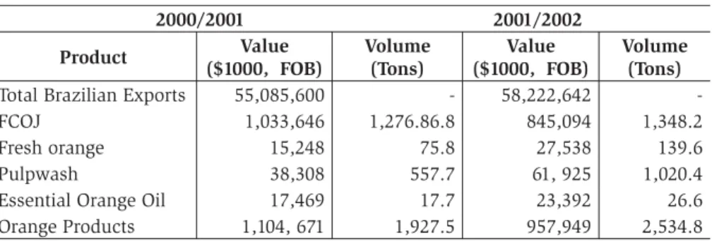
orange products are FCOJ. In 2001/2002, despite the fact that the volume of orange product exports in general (and of FCOJ in particular) grew, the share of those products in total exports, in value terms, went down (from 2% to 1.6%). The fall in the international price for FCOJ helps to explain this. Indeed, FCOJ has been facing low quotations, high stocks and excess of supply in recent years.
Table 7 – Brazilian exports of orange products
2000/2001 2001/2002
Product Value ($1000, FOB)
Volume (Tons)
Value ($1000, FOB)
Volume (Tons)
Total Brazilian Exports 55,085,600 - 58,222,642
-FCOJ 1,033,646 1,276.86.8 845,094 1,348.2
Fresh orange 15,248 75.8 27,538 139.6
Pulpwash 38,308 557.7 61, 925 1,020.4
Essential Orange Oil 17,469 17.7 23,392 26.6
Orange Products 1,104, 671 1,927.5 957,949 2,534.8
Source: CONAB, Feb/2002
The European Union is the main market for Brazilian FCOJ exports. Exports to Europe amount to 69% of the total, and the USA market accounts for the another 21% of Brazilian FCOJ exports. The share of the US market fell during the 90s as a result of competition from Mexican exports, which benefited from lower barriers established within the NAFTA agreement. Table 8 shows the destination of Brazilian FCOJ exports.
Table 8 – Brazilian FCOJ exports - 2000/2001
EU NAFTA ASIA OTHERS TOTAL
Tons 845,781 264,674 99,176 24,643 1,234,274
Share (%) 68.5 21.4 8.0 2.1 100.0
Source: Abecitrus
country in the orange juice market, and about one fifth of its exports go the USA market.
The USA is the largest market for orange juice and the second largest producer. USA producers export part of their output, mainly to Europe, but domestic consumption requires imports of FCOJ, mainly from Brazil and from Mexico. In 2001, USA were responsible for 41.3% and 33.6% of world-wide FCOJ imports, in terms of quantity and value, respectively. Overall, the trade balance for orange juice in the USA is negative.
Lastly, table 9 shows the countries of origin of US FCOJ imports. For the purposes of this study, the most important point to note is the importance of Brazil as a source of the USA’s FCOJ imports. Mexico is also an important player, and, as mentioned above, it has benefited from import tax reductions within NAFTA.
Table 9 – USA orange juice imports: main countries of origin: Jan-Dec 2001
Countries Value* ($) Participation (%)
Brazil 115,071,979 50.90
Costa Rica 39,897,513 17.65
Mexico 39,827,249 17.62
Honduras 5,302,565 2.34
Canada 4,214,873 1.86
Others 21,759,462 9.60
Total 226,073,641 100
Source: Florida Department of Citrus *FOB cost of product
2.2. FCOJ protection in MERCOSUR and the USA
MERCOSUR´s common external tariff (CET) for orange juice is currently 15%. However, given the high competitiveness of Brazilian production, tariff protection is not really necessary to prevent imports of orange products. This means that the lowering of tariffs can be used by Brazil as an important bargaining instrument in current trade negotiations.
from Brazil faces barriers in the form of a per unit tax equivalent to a 56.7%ad valorem tax.
It may be useful to explain how per unit tax adopted by the USA is translated into a percentage of the price of FCOJ, or into an ad
valorem tax. The ad valorem tax imposed by the USA on the orange
juice imported from Brazil is calculated from the per unit tax levied on
thereconstituted orange juice. In the American market, per unit tax is
$0.0785 per liter of reconstituted orange juice ready for consumption. This tax does not change when there are fluctuations in the prices of the product, therefore its ad valorem equivalent is higher when prices are low. The calculation of the ad valorem equivalent factor is based on two parameters: 1) the average price of orange juice, and 2) the conversion factor of concentrated for reconstituted juice. In this study, Hemispheric Database/FTAA V.1.0. parameters were adopted, generating an ad
valorem equivalent factor of 56.7% for FCOJ.
In addition, in the State of Florida, the Brazilian product had to pay another excise tax of 0.027 dollars per gallon ($40/ton) as an equalization tax. The tax imposed by the State of Florida was challenged in court by importers, and as a result, in April 2002, the Florida Citrus Commission was ordered to propose a remedy in the equalization tax case. The court ruled that the equalization tax was unconstitutional because it illegally discriminated against foreign citrus products imported into Florida while exempting juice products imported from other states, mainly from California. As a result of the court’s ruling, the Florida legislature abolished tax exemption for domestic juice, with the new law taking effect in July 2002. Brazil asked for consultations under the WTO, and discussions were opened between Brazilian and US officials.
Brazilian FCOJ competes directly with Mexican exports in the USA market. The FCOJ imports from Mexico pay taxes equivalent to a 30.7%
ad valorem tax.
The most probable outcome of barrier reductions resulting from negotiations within FTAA and/or with the European Union would be an increase in international prices and an increase in FCOJ imports.
Brazil accounts for almost all FCOJ imports in that continent. On the other hand, in the USA market there will be room for a considerable increase in the Brazilian share of FCOJ sales, after US and Mexican output adjust to the new situation.
Overall, the global market for FCOJ can be considered as a textbook case of the impact of trade barriers on output, on trade and on international price formation. In particular, a reduction in the trade barriers faced by Brazilian exporters in the North American FCOJ market would induce an increase in international prices and imports. As a result, Brazilian exporters would benefit from higher prices and from an increase in their share of the American market.3 These issues will be addressed in the
sections below, in a simulation using a partial equilibrium model.
3. The theoretical model and methodological aspects
3.1. Overview of the partial equilibrium approach
In order to calculate the welfare and distributional effects of a reduction in trade barriers in the American FCOJ market, and, for our purposes, the potential rise in Brazilian FCOJ exports to the USA, a version of Hufbauer and Elliot’s4 partial equilibrium model of imperfect
substitutes with perfect competitive markets is used.
Compared to computable general equilibrium models, the partial equilibrium models have two evident advantages: they are less complex and more transparent. Moreover, when the goal is the treatment of a single market at a very detailed level, a partial equilibrium model is often the only feasible way to proceed.
The different generations of partial equilibrium models share at least two common assumptions.
Firstly, in a partial equilibrium model, the impact of a change in the market under investigation is assumed not to disturb related
3 Moreover, in the short run, following an increase in international prices in the American
market, one can imagine that part of Brazil’s FCOJ production to the EU markets would drift to the USA. Therefore, the FCOJ international price in EU markets would increase as a consequence of the supply shortage, and this would benefit Brazilian exporters.
markets. However, this is not to say that the related markets are solemnly ignored. As Francois (1997) rightly stated, the price elasticity of demand included in these models is conceived to reflect underlying linkages between related markets, even though in the implementation of a partial equilibrium model such linkages are sterilized.
Secondly, in a partial equilibrium model, the income effects that arise from a trade policy change are not considered. As a consequence, the demand functions used in these models are represented as being dependent only on prices and not on income, which is treated as an exogenous variable.
Broadly speaking, partial equilibrium models can be classified according to: a) the degree of substitutability of the domestic and imported good; b) the specification of the import supply function; c) the choice of implementation of the model in a linear or non-linear form.
The first distinction divides partial equilibrium models according to the degree of substitutability of the domestically produced and imported good in perfect substitutes and imperfect substitutes models.
On the one hand, in the less complex perfect substitutes model, the imported and domestic goods are considered to be perfectly homogeneous from the consumers’ point of view. In this case, the import demand function is simply defined as the difference between consumption and domestic production, and therefore all the analysis is conducted in the import market. Nevertheless, as suggested by Bowen (1998), in spite of the attractiveness of these models, the assumption of perfect substitutes is generally not consistent with empirically estimated values of the price elasticity of demand.
On the other hand, in the imperfect substitutes model, the domestic and imported goods are considered to be non homogeneous in the eyes of the consumer. The practical consequence of this notion is that in these models there are two different demand functions, one for the domestically produced good and another for the imported good, both dependent on the internal prices of the domestic and imported goods. Therefore, when analyzing the impact of the reduction in tariffs, it is necessary to take into account the repercussion in the two connected markets.
of the foreign exporter country. If the exporter is a big player in the domestic and international market, it is tempting to assume that its supply schedule is flat, i.e. perfectly elastic. Such a model is known as a small country model because it is understood that the importer country is unable to influence the prices of the imported good. In contrast, in a large country model, it is assumed that the importer country is large and therefore able to influence the prices of goods on world markets. If this is the case, the import supply function will be positively sloped, and thus the magnitude of the change in world price and volume of imports will depend significantly on the elasticity of foreign export supply.
Finally, the last difference between partial equilibrium models has to do with the particular mode of their computational implementation. Generally, the functions used in these models are supposed to have constant elasticity. All that has to be done is to solve the system of equations for prices and then use the solution to solve them for quantities.
If a linear approximation is chosen, all the equations can be easily derived in log form. This results in a simpler procedure to solve the problem. However, as Francois & Hall (1997) pointed out, using a linear model, even in a single market, leads to a linearization error that becomes larger when policy changes are significant.
The alternative procedure is to solve the equations in prices and quantities in a non-linear system, i.e. without using the equations in log form. Although in this way the linearization error is minimized, the price to be paid for this is a higher degree of computational complexity.
3.2. The structure and implementation of large country models
3.2.1. Large country models
The implementation of a large country model is very similar to that of small country model. The main difference resides in the assumption that the importer country is large and hence able to influence the prices of goods on world markets. If this is the case, the supply function of the imported good will be positively sloped and therefore the magnitude of the change in world price and volume of imports will depend significantly on the price elasticity of the supply of the imported good.
The system of equations is summarized below. The domestically produced good and its imported substitute are designated by the indexes
d and m.
where
D
d and Dm are the quantities consumed of good d and mrespectively;
S
d andS
m are, respectively, the quantities produced of goodd and m;p
d andp
mare the internal prices of good d and m; is the own-price elasticity of demand of good d; is the cross-price elasticity of demand of good d in relation to good m;E
s is the price elasticity of supply of good d; is the own-price elasticity of demand of good m; is the cross-price elasticity of demand of good m in relation to good d; is the price elasticity of supply of good m; p*isthe world export price; t is the level of tariffs.
demand and supply functions and the equilibrium condition in the market of the imported good.
This system of seven independent equations can be easily solved to generate values for seven endogenous variables,
D
d,
S
d,
P
d,
P
m,
P
*
,
D
mand
S
m.
A change in the level of the tariff allows the calculation of the new endogenous variables. Needless to say, if the exercise imposes a complete elimination of the initial tariff, the value of the final internal price of the imported good (
p
m'
) will be equal to the price received by the importer (p*') and in this case, the fourth equation is redundant.It is important to say that for the implementation of this model it is crucial to know the values of all exogenous variables, i.e. the elasticities and initial quantities of domestic production and import, and the internal prices of the domestic and imported good.
The following graph represents the market for the imported good and the modifications that occur once the tariff is altered.
Graph 1. Effects of removing a trade barrier in the market of the imported good
qm qm´ p*
pm
D’m(pd´ , pm ) Dm(pd , pm) t
E1
E´
u
S
p*’ = pm’
E2
When the tariff is completely eliminated, the subsequent decrease in the price of the imported good induces a fall in the demand schedule in the market for the domestically produced good. The modifications in terms of prices, quantities and welfare in the market for the domestically produced good are the same as before.
Conversely, the consequent decline in the price of the domestic good causes a shift to the left of and below the demand schedule of the imported good represented in graph 1, by the new demand schedule Dm’. The final outcome is an increase in quantity, and the same price for the exporter and for the American consumer. This new price prevailing for both the exporter and the American consumer will lie between the initial prices
p
mand
p
*
.The final step involves understanding how to compute the welfare effects in the market for imported good using graph 1.
Once the importer country influences prices on world markets, the impact in terms of welfare of a tariff reduction will be distributed between three agents: consumers, government and foreign exporters.
With the complete elimination of a tariff (the analysis is similar when the tariff is partially reduced), consumers gain with lower prices and larger quantities. The consumer surplus equals the area of the trapezium
p
m,
E
1,
E
'
,
p
*
'
.
Exporters will also benefit from higher prices and increased quantities, and their surplus can be measured by the area of the trapeziump
*
'
,
E
'
,
E
2,
p
*
. Finally, the government loses tariff revenues equal to the area of the rectanglep
m,
E
1,
E
2,
p
*
.3.2.2. Estimation of elasticities and calibration of parameters
where
S
1 is the share in volume of the domestic product in consumption andS
2 is the share by quantity of imports in consumption;S
is the elasticity of substitution between the domestic and imported good;E
T is the price elasticity of total demand.After calculating the values of the own-price elasticities of demand, the cross-price elasticities in the CES case can be obtained following a methodology proposed by Tarr (1990):
Once all the elasticities are obtained, the next step can be taken. The calibration of the model consists in calculating the values of the
constants in equations (1), (2), (5) and (6). The
procedure for calculating the constants is easily performed with the initial values of quantities and prices assuming that the start situation expresses an undistorted equilibrium.
Finally, when this task is completed, the model is ready to be implemented.
4. Results
In order to estimate the impact of tariff reductions in the American FCOJ market in terms of resource allocation and welfare implications, a partial equilibrium model of imperfect substitutes are used, considering the domestic American FCOJ market a large country. The results are presented in the next section. Besides, two different scenarios for the evaluation of the impact of liberalization in the US FCOJ market were constructed.
scenario evaluates the impact of a partial reduction in the ad valorem
tax to the same level as that applicable on Mexican exports of FCOJ to the USA. The second scenario is considered to be far more realistic because by joining the FTAA, Brazil will most probably benefit more from the same market access conditions than Mexico.
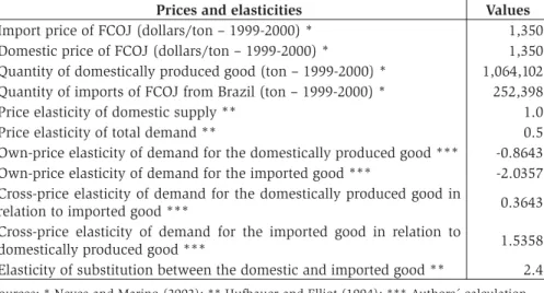
The following table summarizes the initial values of prices and quantities in the years 1999-2000, and the values of all relevant elasticities.
Table 10 – Initial prices, quantities and elasticities
Prices and elasticities Values
Import price of FCOJ (dollars/ton – 1999-2000) * 1,350
Domestic price of FCOJ (dollars/ton – 1999-2000) * 1,350
Quantity of domestically produced good (ton – 1999-2000) * 1,064,102 Quantity of imports of FCOJ from Brazil (ton – 1999-2000) * 252,398
Price elasticity of domestic supply ** 1.0
Price elasticity of total demand ** 0.5
Own-price elasticity of demand for the domestically produced good *** -0.8643 Own-price elasticity of demand for the imported good *** -2.0357 Cross-price elasticity of demand for the domestically produced good in
relation to imported good *** 0.3643
Cross-price elasticity of demand for the imported good in relation to
domestically produced good *** 1.5358
Elasticity of substitution between the domestic and imported good ** 2.4
Sources: * Neves and Marino (2002); **.Hufbauer and Elliot (1994); *** Authors´ calculation.
It is important to point out that in this study, the domestic FCOJ price is considered to be the same as the import price, tariffs included. This is because FCOJ is a relatively homogeneous good, which is extensively traded in commodity markets. Hence, both the domestic and the import price are simply the price of FCOJ in commodity markets.
following table, columns A, B, C and D present the results when this elasticity is equal to 0.5, 1, 2 and 3 respectively.5
Table 11 – Scenario I - Complete elimination of the 56.7% tariff in the FCOJ market
Welfare effects Values (in millions of dollars)
A B C D
Consumer surplus gain 63.32 104.74 156.12 186.91
Producer surplus loss 27.65 44.64 64.42 75.59
Tariff revenue loss 123.29 123.29 123.29 123.29
Efficiency gain -87.62 -63.19 -31.60 -11.97
Efficiency gain / Sales of the imported good (%) * 25.71 18.55 9.27 3.51
Welfare of the exporter 99.37 83.52 63.53 51.34
Change in the price of the domestic good (%) -1.94 -3.16 -4.59 -5.41
Change in the price of the imported good (%) -9.56 -15.14 -21.37 -24.76
Change in the quantity of domestic good (%) -1.94 -3.16 -4.59 -5.41
Change in the quantity of imported good (%) 19.05 32.97 51.80 63.86
Change in the export price (%) 41.72 32.97 23.21 17.89
* Sales of the imported good are measured in the initial situation, before liberalization. This value is calculated by multiplying the initial price of the imported good by the quantity of imports.
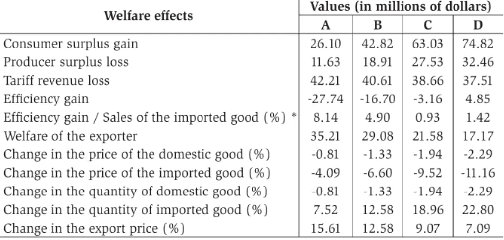
Table 12 shows the welfare effects and percentage changes in prices and quantities in the scenario of a partial reduction of barriers to levels equivalent to a 30% ad valorem tax. It is worth to note that the impacts of a reduction in tariffs are losses of welfare in the local economy, except in the case of a partial reduction of the tariff when the export supply price elasticity of the imported good is equal to 3. The reason for this is straightforward. When the importer country has the power to affect
5 A recent IPEA´s paper is devoted to estimating the supply export functions of several
the world prices, the taxes imposed in the market of imported good are partially paid by the exporter country. So, in the scenario of complete elimination of tariffs, the government loses all its revenue, part of which is driven to the foreign exporter country.6
Table 12 – Scenario II - Partial reduction of the tariff in the FCOJ market to the level of 30%
Welfare effects Values (in millions of dollars)
A B C D
Consumer surplus gain 26.10 42.82 63.03 74.82
Producer surplus loss 11.63 18.91 27.53 32.46
Tariff revenue loss 42.21 40.61 38.66 37.51
Efficiency gain -27.74 -16.70 -3.16 4.85
Efficiency gain / Sales of the imported good (%) * 8.14 4.90 0.93 1.42
Welfare of the exporter 35.21 29.08 21.58 17.17
Change in the price of the domestic good (%) -0.81 -1.33 -1.94 -2.29 Change in the price of the imported good (%) -4.09 -6.60 -9.52 -11.16 Change in the quantity of domestic good (%) -0.81 -1.33 -1.94 -2.29 Change in the quantity of imported good (%) 7.52 12.58 18.96 22.80
Change in the export price (%) 15.61 12.58 9.07 7.09
* Sales of the imported good are measured in the initial situation, before liberalization. This value is calculated by multiplying the initial price of the imported good by the quantity of imports.
The final result in terms of national welfare depends on comparing the government’s losses and the gains incorporated by consumers. As a matter of fact, with unchanged price elasticity of total demand, the more elastic the supply of the imported good, the smaller the government’s losses will be and the larger the consumer surplus. There is always a critical point in terms of the elasticity of supply of the imported good when the losses turn into gains in terms of welfare.
5. Conclusions
The analysis of the potential impact of trade liberalization suggests that strong resistance to trade liberalization is bound to arise in the US
6 Graphs 1 and 2 in the appendix show the principal results in terms of welfare and
FCOJ market. Even in the scenario where trade liberalization maintains the levels of protection currently applied to Mexican exports, the Brazilian producers’ cost advantages would result in a sharp fall in prices and, consequently, in domestic producers’ losses.
Moreover, tariff reduction will cause losses of welfare in the local economy. As explained above, when the importer country affects world prices, a tariff reduction represents a transfer of revenue from local government to foreign producers. Thus, in this case, the more inelastic the supply of the imported good or the greater the tariff reduction, the larger the exporter’s welfare gain will be.
It is important to point out that the results in terms of welfare and changes in prices and quantities are very sensitive to elasticity values. Although this could be thought of as a weakness in partial equilibrium models, they are still a very important tool for evaluating alternative commercial policies. The great sensitivity of these models with regard to elasticity values also suggests that further sectoral studies that emphasize estimating the elasticities utilized in this kind of model would be valuable.
Finally, as mentioned in the introduction to this article, sectors in which domestic producers perceive competitive gaps as being relatively large, and where trade barriers are currently high, are natural candidates to show strong resistance to trade liberalization. This seems certainly to be the case for the FCOJ market in the USA. Anticipating such resistance, Brazilian producers have been investing in the US market, building orange juice processing capacity to become large buyers of both domestically produced and imported FCOJ. Foreign direct investment (FDI) is seen by Brazilian producers as an alternative way of circumventing trade barriers and entering the US market. FDI in this sector seems to demonstrate that Brazilian FCOJ producers do expect strong resistance to trade liberalization from their US counterparts.
6. Bibliography
Bowen, H.P., Hollander, A. and Viaene, J.M. (1998), Applied International Trade Analysis, Macmillan, UK.
Camargo Barros, G.S., Bacchi, M.R.P and Burnquist, H.L. (2002), “Estimação de equações de oferta de exportação de produtos agropecuários para o Brasil, 1992-2000”, IPEA, Texto para Discussão 865, Brasília, Brasil,
Francois, J.F. and Hall, H.K. (1997), “Partial Equilibrium Modeling”, in Francois, J. F. and Reinert, K.A. (eds), Applied Methods for Trade Policy Analysis - A Handbook, Cambridge University Press, UK.
Helpman, E. and Krugman, P.R. (1989), Trade Policy and Market Structure, the MIT Press, USA.
Hufbauer, G.C. and Elliot, K.A. (1994), Measuring the Cost of Protection in the United States, Institute for International Economics, Washington, DC.
Neves, M.F. and Marino, M.K. (2002), Estudo da Competitividade de Cadeias Integradas – Impacto das Zonas de Livre Comércio: cadeia citros, nota técnica final.
Pozzan, M., Muraro, R. and Ueta, F.Z. (2002), “Realidades Distintas”,
Agroanalysis: Revista de Agronegócios da FVG, agosto.
Tarr, D. (1990), “A modified Cournot aggregation condition for obtaining estimates of cross elasticities of demand”, Eastern Economic Journal, 16 (3), 257-264.