ISSN 0101-8205 www.scielo.br/cam
A modified parametric iteration method
for solving nonlinear second order BVPs
ASGHAR GHORBANI, MORTEZA GACHPAZAN∗
and JAFAR SABERI-NADJAFI
Department of Applied Mathematics, School of Mathematical Sciences, Ferdowsi University of Mashhad, Mashhad, Iran
E-mails: [email protected] / [email protected]
Abstract. The original parametric iteration method (PIM) provides the solution of a nonlinear
second order boundary value problem (BVP) as a sequence of iterations. Since the successive iterations of the PIM may be very complex so that the resulting integrals in its iterative relation may not be performed analytically. Also, the implementation of the PIM generally leads to calculation of unneeded terms, which more time is consumed in repeated calculations for series solutions. In order to overcome these difficulties, in this paper, a useful improvement of the PIM is proposed. The implementation of the modified method is demonstrated by solving several nonlinear second order BVPs. The results reveal that the new developed method is a promising analytical tool to solve the nonlinear second order BVPs and more promising because it can further be applied easily to solve nonlinear higher order BVPs with highly accurate.
Mathematical subject classification: Primary: 34B15; Secondary: 41A10.
Key words:modified parametric iteration method, parametric iteration method, second-order
boundary value problems, numerical method.
1 Introduction
In this paper, we investigate the approximate analytical solution of the nonlinear second order BVPs of the type (with this assumption that the problem has the
unique solution on[a,b])
u′′ =F(x,u,u′),
u(a)=α, u(b)=β,
(1)
by a new easy-to-use algorithm proposed in this work, which is based on the parametric iteration method (PIM) [1, 5]. Herea,b, α andβ are the real con-stants and F is a nonlinear continuous operator with respect to its arguments. These BVPs arise in engineering, applied mathematics and several branches of physics, and have attracted much attention. However, it is difficult to ob-tain closed-form solutions for BVPs, especially for nonlinear problems. In most cases, only approximate solutions (either numerical solutions or analytical so-lutions) can be expected. Some numerical methods such as finite difference method [4], finite element method [2] and shooting method [8] have been de-veloped for obtaining approximate solutions to BVPs.
2 The basic idea of the PIM
In this section, we describe the PIM for solving the general second-order BVP of (1). Then the local convergence is discussed.
2.1 The PIM
The PIM provides the solution of Eq. (1) as a sequence of approximations. The method gives rapidly convergent successive approximations of the exact solution if such a solution exists, otherwise approximations can be used for numerical purposes. The idea of the PIM is very simple and straightforward. Let X = C2
[a,b], andL andN be the linear and nonlinear operators on X,
respectively. To explain the basic idea of the PIM, we first consider Eq. (1) as below:
L[u(x)] +N[u(x)] = f(x), (2)
whereL with the propertyL[g] ≡ 0 when g ≡ 0 denotes the so-called
aux-iliary linear operator with respect to u, N is a nonlinear continuous operator
with respect touand f(x)is the source term (hereubelongs to the intersection of domainsL and N, i.e. u ∈ X). Then we construct a family of iterative
processes for Eq. (2) as [1, 5]:
L[un
+1(x)−un(x)] =h H(x)A[un(x)], (3)
with the boundary conditions
un+1(a)=α and un+1(b)=β, (4)
where
A[un(x)] =L[un(x)] +N[un(x)] − f(x)
≡u′′n(x)−F x,un(x),u′n(x)
, (5)
The subscriptn denotes thenth iteration, h 6= 0 and H(x) 6= 0 denote the so-called auxiliary parameter and auxiliary function, respectively, which can be identified easily and efficiently by the techniques proposed in this paper. It should be emphasized that though we have the great freedom to choose the auxiliary linear operator L, the auxiliary parameter h, the auxiliary function H(x)and the initial approximation u0(x), which is fundamental to the valid-ity and flexibilvalid-ity of the PIM, we can also assume that all of them are properly chosen so that solution of (3) exists, as will be shown in this paper later. Accordingly, the successive approximations un(x) n ≥ 0 of PIM in the
aux-iliary parameterh will be readily obtained by choosing the zeroth component. Consequently, the exact solution may be obtained by using
u(x)= lim
n→∞un(x). (6)
Let V =
u : u ∈ C2
[a,b] be the solution space and
ek(x) | ek(x) ∈
V andk =0,1,2,∙ ∙ ∙ denote the set of base functions. Hence we can repres-ent the solution in a seriesu(x) = P∞
k=0ckek(x)whereck is a coefficient. As
long as a set of base functions is determined, the auxiliary linear operatorL, the
initial approximationu0(x)and the auxiliary function H(x)must be chosen in such a way that all solutions of the corresponding PIM equations (3) exist and can be expressed by this set of base functions. Now, in order to avoid expensive computational works for solving (1) via the PIM, it is straightforward to use the set of base functions
{(x −a)m |m =0,1,2,∙ ∙ ∙ }, (7)
to representu(x), i.e.,
u(x)=
∞ X
m=0
γm(x−a)m, (8)
whereγm ∈ R(m =0,1,2,∙ ∙ ∙)are coefficients to be determined. In view of
the solution expression (7) and according to the boundary conditions (4), it is straightforward to choose
L[u(x)] =u′′(x), (9)
two terms of the set of base functions, that is, 1 and(x−a))
L[c1(x−a)+c2] =0, (10)
as the auxiliary linear operator where c1 andc2 are integral constants, and to choose an initial approximation ofu(x), which is the solution of the correspond-ing linear homogeneous equationL[u0(x)] =0,
u0(x)=α+ α−β
a−b(x−a). (11)
For simplicity, the auxiliary function H(x) can be chosen in the form
H(x)=1. According to (10), the solution of the PIM equation (3) becomes
un+1(x)=un(x)+h
Z x
a
(x−t)A[un(t)]dt+c1(x−a)+c2, (12)
where A[un(t)] is defined as in (5) and the integral constants c1 and c2 are
determined by imposing the boundary conditions (4). We, therefore, obtain
un+1(x) = un(x)+h
Z x
a
(x −t)A[un(t)]dt
−hx−a b−a
Z b
a
(b−t)A[un(t)]dt,
(13)
where A[un(t)] = u′′
n(t)− F t,un(t),u′n(t)
. Therefore, the successive ap-proximations un(x) (n ≥ 1) of the PIM iterative relationship of (13) in the
auxiliary parameterhwill be readily obtained, especially by means of symbolic computation software such as Maple, Mathematica, Matlab and others.
2.2 Convergence theorem
The parametric iteration formula, (3), makes a recurrence sequence {un(x)}.
Theorem 2.1. Let F be a nonlinear continuous operator and for any positive integer n, un ∈ C2[a,b]. Provided that the sequence(6)uniformly converges,
where un(x)is produced by the parametric iteration formulation of(3), it must
be the exact solution of the problem(1).
Proof. If the sequenceun(x)converges, we can write
U(x)= lim
n→∞un(x), (14)
and it holds
U(x)= lim
n→∞un+1(x). (15)
Using (14), (15) and the definition ofL, we can easily gain
lim
n→∞ Lun
+1(x)−un(x)
=L lim
n→∞
un+1(x)−un(x)
=0. (16)
From (16) and according to (3), we obtain
L lim
n→∞
un+1(x)−un(x)
=h H(x) lim
n→∞
Aun(x)=0. (17)
Sinceh6=0 andH(x)6=0, the relation (17) gives us
lim
n→∞
Aun(x)=0. (18)
From (18) and the continuity ofFoperator, it holds
lim
n→∞
A[un(x)] = lim
n→∞
u′′n(x)−F x,un(x),u′n(x)
= lim
n→∞u ′′
n(x)−F
x, lim
n→∞un(x),nlim→∞u ′
n(x)
(19)
=
lim
n→∞un(x) ′′
−F
x, lim
n→∞un(x),
lim
n→∞un(x) ′
=U′′(x)−F x,U(x),U′(x).
From the equations (18) and (19), we have
On the other hand, in view of (1), (4) and (15), it holds
U(a)= lim
n→∞un+1(a)=α, (21) U(b)= lim
n→∞un+1(b)=β, (22)
Therefore, according to the above expressions, (20)-(22), U(x)must be the exact solution of the problem (1) and this ends the proof.
It is clear that the convergence of the sequence (6) depends upon the initial guessu0(x), the auxiliary linear operatorL, the auxiliary parameterh and the auxiliary function H(x). Fortunately, the PIM provides us with great freedom of choosing them. Thus, as long asu0(x),L,handH(x)are so properly chosen
that the sequence (6) converges in a region a ≤ x ≤ b, it must converge to the exact solution in this region. Therefore, the combination of the conver-gence theorem and the freedom of the choice of above factors establishes the cornerstone of the validity and flexibility of the PIM.
3 A modified PIM
Since the successive iterations of the PIM may be very complex so that the resulting integrals in the relation (13) may not be performed analytically. Also, the implementation of the PIM generally leads to calculation of unneeded terms, which more time is consumed in repeated calculations for series solu-tions. In order to overcome these difficulties, in this section, a useful modifica-tion of the PIM is proposed. To completely eliminate these shortcomings in each step, provided thatA[un(t)]in each of iterations is expanded in Taylor series arounda, we suggest the following improvement of the PIM of (13), which is called the modified PIM (MPIM):
un+1(x)=un(x)+h
Z x
a
(x −t)Gn(t)dt−h
x −a b−a
Z b
a
(b−t)Gn(t)dt, (23)
where
A[un(t)] =Gn(t)+O (t−a)n+1. (24)
straight-forward way. Furthermore, it can reduce the size of calculations. Most impor-tantly, however, it is the fact that the MPIM algorithm (23) may solve a BVP exactly if its solution is an algebraic polynomial up to some degree.
4 Choosing the auxiliary parameterh
It is important to ensure that a solution series obtained using MPIM, which is always as a family of solution expressions in the auxiliary parameterh, is con-vergent in a large enough region whereby the convergence region and rate of solution series are dependent upon the auxiliary parameter h and thus can be enlarged by choosing a proper value forh. Most important, however, it is how to choose the value ofhto make sure that the solution series converges fast enough in a large enough region. Since we have a family of solution expressions in the auxiliary parameterh, hence, regardingh as an independent variable, a simple and practical way of selecting h is to plot the curve of solution’s derivatives with respect to in some points [5, 7]. So, if the solution is unique, all of them converge to the same value and hence there exists a horizontal line segment in its figure that corresponds to a region ofh called the valid region of h. Thus, if we set h any value in the so-called valid region of h, we are sure that the corresponding solution series converges. It is found that, for given initial ap-proximation and the auxiliary function, the valid regions of are often nearly the same for a given problem. In most cases, we can find a proper value of h to ensure that the solution series converges in the whole spatial/temporal regions. Therefore, the curveshprovide us with an easy way to show the influence ofh
on the convergence region and rate of solution series.
5 Results
Example 5.1. As the first example, we consider the following nonlinear sec-ond order BVP [3]:
u′′= 1
2exp
1
2(x+1)cos(u−3x+7)
, (25)
subject to the boundary conditions
u(−1)= −10 and u(1)= −4. (26)
In order to solve the equation (25) using the MPIM algorithm, according to (2), we choose
X =C2[−1,1],
L[u(x)] =u′′,
N[u(x)] = −1
2exp
1
2(x+1)cos(u−3x +7)
and f(x) ≡ 0 which D(L) = D(N) = X. So for this problem u belongs
to the intersection of these domains, i.e. u ∈ X.
Therefore, according to (23) and (24), we have the following MPIM iter-ative formula:
un+1(x)=un(x)+h
Z x −1
(x −t)Gn(t)dt−h
x +1 2
Z 1 −1
(1−t)Gn(t)dt,
where
u′′n(t)−1 2exp
1
2(t+1)cos(un(t)−3t+7)
=Gn(t)+O (t+1)n+1
.
Starting with the initial approximationu0(x)= −10+3(x+1), we get
u1(x)= −10+
3+1 2h
(x+1)− 1
4h(x +1) 2
,
u2(x)= −10+
3+7 6h
(x+1)− 1
4[h+h(1+h)]
(x+1)2− 1
24h(x+1) 3, ..
To investigate the valid regionh of the solution obtained via the 10th-order MPIM, here we plot the curve ofu′(−1) with respect to h, as shown in
Fig-ure 1. According to this curve, it is easy to discover the valid region ofh. We point out that the valid region ofhbecomes more accurate as the numbern in-creases. It is usually convenient to investigate the valid region ofhof the MPIM by means of such kinds of the curves.
−1.8 −1.6 −1.4 −1.2 −1 −0.8 −0.6 −0.4 −0.2 0 −2
−1 0 1 2 3 4 5 6 7 8
h
u
′ (−
1
)
Figure 1 – The valid region of the auxiliary parameterh using the 10th-order MPIM for Example 5.1.
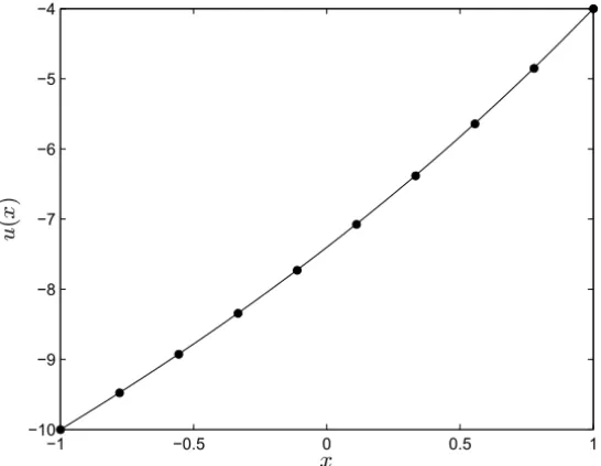
Now, according to (23) and (24), by taking n = 9, we can obtain a 10th-order MPIM approximation of (25) on [−1,1]. Figure 2 shows the approx-imate analytical solution obtained for Eq. (25) by using the 10th-order MPIM forh = −0.5 versus the numerical solution. It must be emphasized that our approximate solution applying the modified method is in excellent agreement with the numerical values.
Example 5.2. As the other example, we consider the following nonlinear second order BVP [3]:
−1 −0.5 0 0.5 1 −10
−9 −8 −7 −6 −5 −4
x
u
(
x
)
Figure 2 – Comparing the numerical solution (circle symbols) with the 10th-order MPIM solution whenh = −0.5 (solid line) for Example 5.1.
subject to the boundary conditions
u(0)=0 and u(1)=0. (28)
In order to solve the equation (27) using the MPIM algorithm, according to (2), we chooseX =C2[0,1],L[u(x)] =u′′,N[u(x)] = −arctan(u)−2uand f(x) =cos(x)which D(L)= D(N)= X. So for this problemu belongs to the intersection of these domains, i.e. u ∈ X.
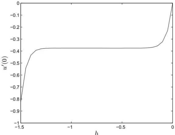
The valid regionh and the approximate analytical solution of the 15th-order MPIM whenh = −0.4 for Eq. (27) have been given in Figures 3 and 4, re-spectively.
Example 5.3. As the other example, we consider the following nonlinear second order BVP [9]:
u′′−s2u−Fsu2+ 1
M =0, (29)
subject to the boundary conditions
−1.5 −1 −0.5 0 −1
−0.9 −0.8 −0.7 −0.6 −0.5 −0.4 −0.3 −0.2 −0.1 0
h
u
′ (0
)
Figure 3 – The valid region of the auxiliary parameterh using the 15th-order MPIM for Example 5.2.
0 0.2 0.4 0.6 0.8 1 −0.1
−0.08 −0.06 −0.04 −0.02 0
x
u
(
x
)
where the parameters are selected as in [9], that is,s =F = M=1.
In order to solve the equation (29) using the MPIM algorithm, according to (2), we chooseX =C2[−1,1],L[u(x)] = u′′,N[u(x)] = −s2u−Fsu2and f(x)= −M1 whichD(L)= D(N)= X. So for this problemubelongs to the
intersection of these domains, i.e. u ∈ X.
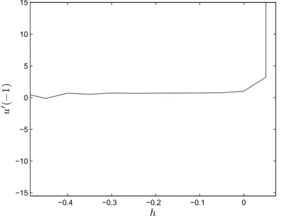
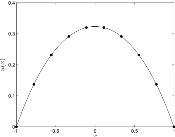
The valid regionh and the approximate analytical solution of the 25th-order MPIM when h = −0.25 for Eq. (29) have been given in Figures 5 and 6, respectively.
−0.4 −0.3 −0.2 −0.1 0 −15
−10 −5 0 5 10 15
h
u
′ (−
1
)
Figure 5 – The valid region of the auxiliary parameterh using the 25th-order MPIM for Example 5.3.
It is interesting to point out that the MPIM algorithm proposed in this work is capable of solving the nonlinear second order BVPs of the general form
F x,u,u′,u′′
=0 subject to the boundary conditionsu(a)=αandu(b)=β. For instance see the following example (Example 5.4).
Example 5.4. As the final example, we consider the following nonlinear sec-ond order BVP:
−1 −0.5 0 0.5 1 0
0.1 0.2 0.3 0.4
x
u
(
x
)
Figure 6 – Comparing the numerical solution (circle symbols) with the 25th-order MPIM solution whenh = −0.25 (solid line) for Example 5.3.
subject to the boundary conditions
u(−1)=1 and u(4)=16. (32)
with the exact solutionu(x)=x2.
In order to solve the equation (31) using the MPIM algorithm, according to (2), we choose
X =C2[−1,4], L[u(x)] =u′′, N[u(x)] =√532+2xu′−2uu′′
and f(x) ≡ 0 which D(L) = D(N) = X. So for this problemu belongs to
the intersection of these domains, i.e. u ∈ X.
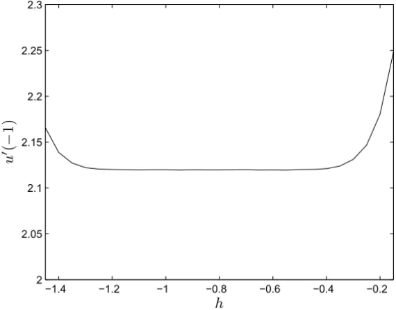
The valid regionh and the approximate analytical solution of the 10th-order MPIM whenh = −1 for Eq. (31) have been given in Figures 7 and 8, respec-tively.
−1.4 −1.2 −1 −0.8 −0.6 −0.4 −0.2 2
2.05 2.1 2.15 2.2 2.25 2.3
h
u
′ (−
1
)
Figure 7 – The valid region of the auxiliary parameterh using the 10th-order MPIM for Example 5.4.
−1 0 1 2 3 4 0
2 4 6 8 10 12 14 16
x
u
(
x
)
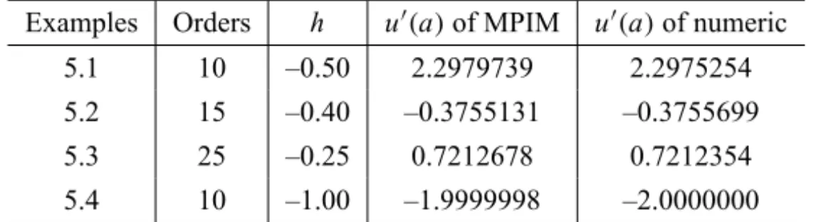
Examples Orders h u′(a)of MPIM u′(a)of numeric
5.1 10 –0.50 2.2979739 2.2975254
5.2 15 –0.40 –0.3755131 –0.3755699
5.3 25 –0.25 0.7212678 0.7212354
5.4 10 –1.00 –1.9999998 –2.0000000
Table 1 – Comparison of the values of the MPIM approximate solution foru′(a) with the numerical solution.
Examples Orders h u′(b)of MPIM u′(b)of numeric
5.1 10 –0.50 3.9834993 3.9741175
5.2 15 –0.40 0.3011200 0.3013059
5.3 25 –0.25 –0.721417 –0.721235
5.4 10 –1.00 7.9999991 8.0000000
Table 2 – Comparison of the values of the MPIM approximate solution for u′(b) with the numerical solution.
6 Conclusions
In this study we have proposed an effective modification of the parametric iter-ation method called the modified PIM (MPIM) to solve nonlinear second order boundary value problems. The obtained results demonstrate that the MPIM is easy to implement, accurate when applied to the nonlinear second order BVPs and avoid tedious computational works. Moreover, it can further be employed easily to solve nonlinear higher order BVPs with highly accurate.
Acknowledgments. The authors would like to express their sincere thanks to the reviewers for the careful reading of the manuscript and giving their valu-able comments which helped to improve it considerably.
REFERENCES
[1] A. Ghorbani, Toward a new analytical method for solving nonlinear fractional
differential equations. Comput. Meth. Appl. Mech. Engrg.,197(2008), 4173–4179.
[2] A.G. Deacon and S. Osher, Finite-element method for a boundary-value problem
[3] D.R. Kincaid and E.W. Cheny, Numerical Analysis Mathematics of Scientific
Computing. California, Brooke Cole (2001).
[4] E. Doedel, Finite difference methods for nonlinear two-point boundary-value
problems. SIAM J. Numer. Anal,16(1979), 173–185.
[5] J. Saberi-Nadjafi and A. Ghorbani, Piecewise-truncated parametric iteration
method: a promising analytical method for solving Abel differential equations.
Z. Naturforsch.65a(2010), 529–539.
[6] S. Liang and D.J. Jeffrey, Approximate solutions to a parameterized sixth order
boundary value problem. Comput. Math. Appl.,59(2010), 247–253.
[7] Sh.J. Liao, Beyond perturbation: Introduction to the Homotopy Analysis Method. Boca Raton, Chapman & Hall/CRC Press (2003).
[8] S.M. Roberts and J.S. Shipman, Two Point Boundary Value Problems: Shooting
Methods. American Elsevier, New York (1972).
[9] S.S Motsa, P. Sibanda and S. Shateyi, A new spectral-homotopy analysis method
for solving a nonlinear second order BVP. Commun. Nonlinear Sci. Numer.