Behavior Emergence in Autonomous Robot
Control by Means of Feedforward and Recurrent
Neural Networks
Stanislav Sluˇsn´
y, Petra Vidnerov´
a, Roman Neruda
∗Abstract—We study the emergence of intelligent behavior within a simple intelligent agent. Cognitive agent functions are realized by mechanisms based on neural networks and evolutionary algorithms. The evolutionary algorithm is responsible for the adap-tation of a neural network parameters based on the performance of the embodied agent endowed by dif-ferent neural network architectures. In experiments, we demonstrate the performance of evolutionary al-gorithm in the problem of agent learning where it is not possible to use traditional supervised learning techniques. A comparison of different networks archi-tectures is presented and discussed.
Keywords: Robot control, Evolutionary algorithms, Neural networks, Behavior emergence.
1
Introduction
One of the main approaches of Artificial Intelligence is to gain insight into natural intelligence through a synthetic approach, by generating and analyzing artificial intelli-gent behavior. In order to glean an understanding of a phenomenon as complex as natural intelligence, we need to study complex behavior in complex environments.
In contrast to traditional systems, reactive and behav-ior based systems have placed agents with low levels of cognitive complexity into complex, noisy and uncertain environments. One of the many characteristics of intelli-gence is that it arises as a result of an agent’s interaction with complex environments. Thus, one approach to de-velop autonomous intelligent agents, calledevolutionary robotics, is through a self-organization process based on artificial evolution. Its main advantage is that it is an ideal framework for synthesizing agents whose behavior emerge from a large number of interactions among their constituent parts [10].
∗Institute of Computer Science, Academy of Science of the Czech Republic, Pod vod´arenskou vˇeˇz´ı 2, Prague 8, Czech Republic, email: [email protected].
This work has been supported by the the project no. 1ET100300419 of the Program Information Society (of the Thematic Program II of the National Research Program of the Czech Republic) “Intelli-gent Models, Algorithms, Methods and Tools for the Semantic Web Realization”.
In the following sections we introduce multilayer percep-tron networks (MLP), Elman’s networks (ELM) and ra-dial basis function networks (RBF). Then we take a look at Khepera robots and related simulation software. In the following section we present two experiments with Khep-era robots. In both of them, the artificial evolution is guiding the self-organization process. In the first experi-ment we expect an emergence of behavior that guarantees full maze exploration. The second experiment shows the ability to train the robot to discriminate between walls and cylinders. In the last section we draw some conclu-sions and present directions for our future work.
2
Neural Networks
Neural networks are widely used in robotics for various reasons. They provide straightforward mapping from in-put signals to outin-put signals, several levels of adaptation and they are robust to noise.
2.1
Multilayer Perceptron Networks
A multilayer feedforward neural network is an intercon-nected network of simple computing units called neurons which are ordered in layers, starting from the input layer and ending with the output layer [5]. Between these two layers there can be a number of hidden layers. Connec-tions in this kind of networks only go forward from one layer to the next. The outputy(x) of a neuron is defined in equation (1):
y(x) =g n
X
i=1 wixi
!
, (1)
wherexis the neuron withninput dendrites (x0 ... xn),
one output axony(x),w0 ... wn are weights andg:ℜ →
ℜ is the activation function. We have used one of the most common activation functions, the logistic sigmoid function (2):
σ(ξ) = 1/(1 +e−ξt), (2)
Figure 1: Scheme of layers in the Elman network archi-tecture.
In our approach, the evolutionary algorithm is responsi-ble for weights modification, the architecture of the net-work is determined in advance and does not undergo the evolutionary process.
2.2
Recurrent Neural Networks
In recurrent neural networks, besides the feedforward connections, there are additional recurrent connections that go in the opposite direction. These networks are of-ten used for time series processing because the recurrent connection can work as a memory for previous time steps. In the Elman [3] architecture, the recurrent connections explicitly hold a copy (memory) of the hidden units ac-tivations at the previous time step. Since hidden units encode their own previous states, this network can detect and reproduce long sequences in time. The scheme how the Elman network works is like this (also cf. Fig. 1):
• Compute hidden unit activations using net input from input units and from the copy layer.
• Compute output unit activations as usual based on the hidden layer.
• Copy new hidden unit activations to the copy layer.
2.3
Radial Basis Function Networks
An RBF neural network represents a relatively new neu-ral network architecture. In contrast with the multilayer perceptrons the RBF network contains local units, which was motivated by the presence of many local response units in human brain. Other motivation came from nu-merical mathematics, radial basis functions were first in-troduced as a solution of real multivariate interpolation problems [13].
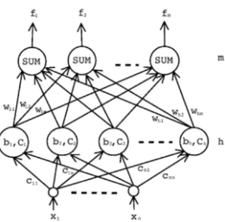
The RBF network is a feed-forward neural network with one hidden layer of RBF units and a linear output layer
Figure 2: RBF network architecture
(see Fig. 2). By the RBF unit we mean a neuron with
n real inputs~xand one real output y, realizing a radial basis functionϕ, such as Gaussian:
y(~x) =ϕ
k~x−~ck
b
. (3)
The network realizes the function:
fs(~x) = h
X
j=1 wjsϕ
k~x−~cjk bj
, (4)
wherefsis the output of the s-th output unit.
There is a variety of algorithms for RBF network learn-ing, in our previous work we studied their behavior and possibilities of their combinations [8, 9].
The learning algorithm that we use for RBF networks was motivated by the commonly used three-step learn-ing [9]. Parameters of RBF network are divided into three groups: centers, widths of the hidden units, and output weights. Each group is then trained separately. The centers of hidden units are found by clustering (k-means algorithm) and the widths are fixed so as the ar-eas of importance belonging to individual units cover the whole input space. Finally, the output weights are found by EA. The advantage of such approach is the lower num-ber of parameters to be optimized by EA , i.e. smaller length of individual.
3
Evolutionary Learning Algorithms for
Robotics
3.1
The Khepera Robot
two on other side. In “active mode” these sensors emit a ray of infrared light and measure the amount of reflected light. The closer they are to a surface, the higher is the amount of infrared light measured. The Khepera sen-sors can detect a white paper at a maximum distance of approximately 5 cm.
In a typical setup, the controller mechanism of the robot is connected to the eight infrared sensors as input and its two outputs represent information about the left and right wheel power. For a neural network we typically con-sider architectures with eight input neurons, two output neurons and a single layer of neurons, mostly five or ten hidden neurons is considered in this paper. It is difficult to train such a network by traditional supervised learn-ing algorithms since they require instant feedback in each step, which is not the case for evolution of behavior. Here we typically can evaluate each run of a robot as a good or bad one, but it is impossible to assess each one move as good or bad. Thus, the evolutionary algorithm represent one of the few possibilities how to train the network.
3.2
Evolutionary Algorithm
The evolutionary algorithms (EA) [6, 4] represent a stochastic search technique used to find approximate so-lutions to optimization and search problems. They use techniques inspired by evolutionary biology such as mu-tation, selection, and crossover. The EA typically works with a population of individuals representing abstract representations of feasible solutions. Each individual is assigned a fitness that is a measure of how good solu-tion it represents. The better the solusolu-tion is, the higher the fitness value it gets. The population evolves towards better solutions. The evolution starts from a population of completely random individuals and iterates in genera-tions. In each generation, the fitness of each individual is evaluated. Individuals are stochastically selected from the current population (based on their fitness), and mod-ified by means of operators mutation and crossover to form a new population. The new population is then used in the next iteration of the algorithm.
3.3
Evolutionary Network Learning
Various architectures of neural networks used as robot controllers are encoded in order to use them the evolu-tionary algorithm. The encoded vector is represented as a floating-point encoded vector of real parameters deter-mining the network weights.
Typical evolutionary operators for this case have been used, namely the uniform crossover and the mutation which performs a slight additive change in the parameter value. The rate of these operators is quite big, ensuring the exploration capabilities of the evolutionary learning. A standard roulette-wheel selection is used together with a small elitist rate parameter. Detailed discussions about
Figure 3: In the maze exploration task, agent is rewarded for passing through the zone, which can not be sensed. The zone is drawn as the bigger circle, the smaller circle represents the Khepera robot. The training environment is of 60x30 cm.
the fitness function are presented in the next section.
4
Experiments
4.1
Setup
Although evolution on real robots is feasible, serial eval-uation of individuals on a single physical robot might require quite a long time. One of the widely used ulation software (for Khepera robots) is the Yaks sim-ulator [2], which is freely available. Simulation consists of predefined number of discrete steps, each single step corresponds to 100 ms.
To evaluate the individual, simulation is launched several times. Individual runs are called “trials”. In each trial, neural network is constructed from the chromosome, envi-ronment is initialized and the robot is put into randomly chosen starting location. The inputs of neural networks are interconnected with robot’s sensors and outputs with robot’s motors. The robot is then left to “live” in the simulated environment for some (fixed) time period, fully controlled by neural network. As soon as the robot hits the wall or obstacle, simulation is stopped. Depending on how well the robot is performing, the individual is eval-uated by value, which we call “trial score”. The higher the trial score, the more successful robot in executing the task in a particular trial. The fitness value is then obtained by summing up all trial scores.
4.2
Maze Exploration
In this experiment, the agent is put in the maze of 60x30 cm. The agent’s task is to fully explore the maze. Fitness evaluation consists of four trials, individual trials differ by agent’s starting location. Agent is left to live in the environment for 250 simulation steps.
The three-component Tk,j motivates agent to learn to
move and to avoid obstacles:
Tk,j=Vk,j(1−
p
Figure 4: The agent is put in the bigger maze of 100x100 cm. Agent’s strategy is to follow wall on it’s left side.
First component Vk,j is computed by summing absolute
values of motor speed in thek-th simulation step andj -th trial, generating value between 0 and 1. The second component (1−p
∆Vk,j) encourages the two wheels to
rotate in the same direction. The last component (1−
ik,j) encourage obstacle avoidance. The valueik,j of the
most active sensor in k-th simulation step andj-th trial provides a conservative measure of how close the robot is to an object. The closer it is to an object, the higher the measured value in range from 0 to 1. Thus,Tk,j is in
range from 0 to 1, too.
In thej-th trial, score Sj is computed by summing
nor-malized trial gainsTk,j in each simulation step.
Sj= 250
X
k=1 Tk,j
250 (6)
To stimulate maze exploration, agent is rewarded, when it passes through the zone. The zone is randomly located area, which can not be sensed by an agent. Therefore, ∆j
is 1, if agent passed through the zone in j-th trial and 0 otherwise. The fitness value is then computed as follows:
F itness=
4
X
j=1
(Sj+ ∆j) (7)
Successful individuals, which pass through the zone in each trial, will have fitness value in range from 4 to 5. The fractional part of the fitness value reflects the speed of the agent and it’s ability to avoid obstacles.
4.3
Results
All the networks included in the tests were able to learn the task of finding a random zone from all four positions. The resulting best fitness values (cf. Tab. 1) are all in
0 0.5 1 1.5 2 2.5 3 3.5 4 4.5 5
0 50 100 150 200
fitness
generations RBF network with 5 units
mean max min
Figure 5: Plot of fitness curves in consecutive populations (maximal, minimal, and average individual) for a typical EA run (one of ten) training the RBF network with 5 units.
the range of 4.3–4.4 and they differ only in the order of few per cent. It can be seen that the MLP networks per-form slightly better, RBF networks are in the middle, while recurrent networks are a bit worse in terms of the best fitness achieved. According to their general perfor-mance, which takes into account ten different EA runs, the situation changes slightly. In general, the networks can be divided into two categories. The first one repre-sents networks that performed well in each experiment in a consistent manner, i.e. every run of the evolution-ary algorithm out of the ten random populations ended in finding a successful network that was able to find the zone from each trial. MLP networks and recurrent net-works with 5 units fall into this group. The second group has in fact a smaller trial rate because, typically, one out of ten runs of EA did not produced the optimal solution. The observance of average and standard deviation values in Tab. 1 shows this clearly. This might still be caused by the less-efficient EA performance for RBF and Elman networks.
The important thing is to test the quality of the obtained solution is tested in a different arena, where a bigger maze is utilized (Fig. 4). Each of the architectures is capable of efficient space exploration behavior that has emerged during the learning to find random zone positions. The above mentioned figure shows that the robot trained in a quite simple arena and endowed by relatively small net-work of 5–10 units is capable to navigate in a very com-plex environment.
4.4
Walls and Cylinders Experiment
Network type Maze exploration Wall and cylinder
mean std min max mean std min max
MLP 5 units 4.29 0.08 4.20 4.44 2326.1 57.8 2185.5 2390.0 MLP 10 units 4.32 0.07 4.24 4.46 2331.4 86.6 2089.0 2391.5 ELM 5 units 4.24 0.06 4.14 4.33 2250.8 147.7 1954.5 2382.5 ELM 10 units 3.97 0.70 2.24 4.34 2027.8 204.3 1609.5 2301.5 RBF 5 units 3.98 0.90 1.42 4.36 1986.6 230.2 1604.0 2343.0 RBF 10 units 4.00 0.97 1.23 4.38 2079.4 94.5 2077.5 2359.5
Table 1: Comparison of the fitness values achieved by different types of network in the experiments.
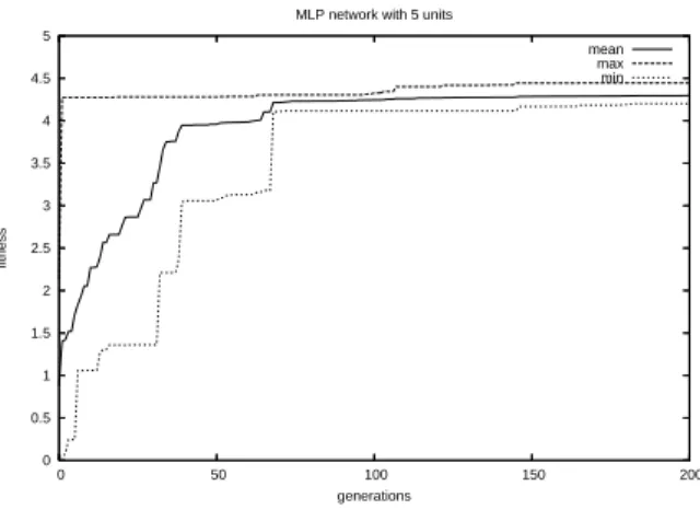
0 0.5 1 1.5 2 2.5 3 3.5 4 4.5 5
0 50 100 150 200
fitness
generations MLP network with 5 units
mean max min
Figure 6: Plot of fitness curves in consecutive populations (maximal, minimal, and average individual) for a typical EA run (one of ten) training the MLP network with 5 units.
Figure 7: Trajectory of an agent doing the Walls and cylinders task. The small circle represents the searched target cylinder. The agent is rewarded in the zone rep-resented by a bigger circle. It is able to discriminate be-tween wall and cylinder, and after discovering the cylin-der it stays in it’s vicinity.
networks which are passively exposed to a set of sensory patterns without being able to interact with the external environment through motor action), are mostly unable to discriminate between different objects. However, this problem can easily be solved by agents that are left free to move in the environment.
The agent is allowed to sense the world by only six frontal infrared sensors, which provide it with only limited infor-mation about environment. Fitness evaluation consists of five trials, individual trials differ by agent’s starting location. Agent is left to live in the environment for 500 simulation steps. In each simulation step, trial score is increased by 1, if robot is near the cylinder, or 0.5, if robot is near the wall. The fitness value is then obtained by summing up all trial scores. Environment is the arena of 40x40 cm surrounded by walls.
4.5
Results
It may seem surprising that even this more complicated task was solved quite easily by relatively simple network architectures. The images of walls and cylinders are over-lapping a lot in the input space determined by the sensors.
The results in terms of best individuals are again quite comparable for different architectures with reasonable network sizes. The differences are more pronounced than in the case of the previous task though. Again, the MLP is the overall winner mainly when considering the overall performance averaged over ten runs of EA. The behavior of EA for Elman and RBF networks was less consistent, there were again several runs that obviously got stuck in local extrema (cf. Tab. 1).
We should emphasize the difference between fitness func-tions in both experiment. The fitness function used in the first experiment rewards robot for single actions, whereas in the second experiment, we describe only desired behav-ior.
5
Conclusions
The main goal of this paper was to demonstrate the abil-ity of neural networks trained by evolutionary algorithm to achieve non-trivial robotic tasks. There have been two experiments carried out with three types of neural net-works and different number of units.
For the maze exploration experiment the results are en-couraging, a neural network of any of the three types is able to develop the exploration behavior. The trained network is able to control the robot in the previously unseen environment. Typical behavioral patterns, like following the right wall have been developed, which in turn resulted in the very efficient exploration of an un-known maze. The best results achieved by any of the network architectures are quite comparable, with sim-pler perceptron networks (such as the 5-hidden unit per-ceptron) marginally outperforming Elman and RBF net-works.
In the second experiment it has been demonstrated that the above mentioned approach is able to take advantage of the embodied nature of agents in order to tell walls from cylindrical targets. Due to the sensor limitations of the agent, this task requires a synchronized use of a suit-able position change and simple pattern recognition. This problem is obviously more difficult than the maze explo-ration, nevertheless, most of the neural architectures were able to locate and identify the round target regardless of its position.
The results reported above represent just a few steps in the journey toward more autonomous and adaptive robotic agents. The robots are able to learn simple be-havior by evolutionary algorithm only by rewarding the good ones, and without explicitly specifying particular actions. The next step is to extend this approach for more complicated actions and compound behaviors. This can be probably realized by incremental learning one net-work a sequence of several tasks. Another—maybe a more promising approach—is to try to build a higher level architecture (like a type of the Brooks subsumption ar-chitecture [1]) which would have a control over switching simpler tasks realized by specialized networks. Ideally, this higher control structure is also evolved adaptively without the need to explicitly hardwire it in advance. The last direction of our future work is the extension of this methodology to the field of collective behavior.
References
[1] Brooks, R. A.: A robust layered control system for a mobile robot. IEEE Journal of Robotics and Au-tomation (1986),RA-2, 14-23.
[2] J. Carlsson, T. Ziemke, YAKS - yet another Khep-era simulator, in: S. Ruckert, Witkowski (Eds.)
Autonomous Minirobots for Research and Entertain-ment Proceedings of the Fifth International Heinz Nixdorf Symposium, HNI-Verlagsschriftenreihe, Paderborn, Germany, 2001.
[3] J. Elman, Finding structure in time,Cognitive Sci-ence 14 (1990) 179-214.
[4] D. B. Fogel.Evolutionary Computation: The Fossil Record. MIT-IEEE Press. 1998.
[5] S. Haykin. Neural Networks: A Comprehensive Foundation (2nd ed). Prentice Hall, 1998.
[6] J. Holland.Adaptation In Natural and Artificial Sys-tems (reprint ed). MIT Press. 1992.
[7] Khepera II web page documentation. http://www.k-team.com
[8] Neruda, R., Kudov´a, P.: Hybrid learning of RBF networks. Neural Networks World, 12 (2002) 573– 585
[9] Neruda, R., Kudov´a, P.: Learning methods for RBF neural networks. Future Generations of Computer Systems,21, (2005), 1131–1142.
[10] S. Nolfi, D. Floreano. Evolutionary Robotics — The Biology, Intelligence and Technology of Self-Organizing Machines. The MIT Press, 2000. [11] S. Nolfi. Adaptation as a more powerful tool than
decomposition and integration. In T.Fogarty and G.Venturini (Eds.), Proceedings of the Workshop on Evolutionary Computing and Machine Learning, 13th International Conference on Machine Learning, Bari, 1996.
[12] S. Nolfi. The power and limits of reactive agents. Technical Report. Rome, Institute of Psychology, National Research Council, 1999.