Abstract
The exact solution for the problem of damped, steady state response, of in-plane Timoshenko frames subjected to harmonically time varying external forces is here described. The solution is obtained by using the classical dynamic stiffness matrix (DSM), which is non-linear and transcendental in respect to the excitation frequency, and by performing the harmonic analysis using the Laplace transform. As an original contribution, the partial differential coupled governing equations, combining displacements and forces, are directly subjected to Laplace transforms, leading to the member DSM and to the equivalent load vector formulations. Additionally, the members may have rigid bodies attached at any of their ends where, optionally, internal forces can be released. The member matrices are then used to establish the global matrices that represent the dynamic equilibrium of the overall framed structure, preserving close similarity to the finite element method. Several application examples prove the certainty of the proposed method by comparing the model results with the ones available in the literature or with finite element analyses.
Keywords
exact harmonic analysis; Laplace transform; Timoshenko beam; dynamic stiffness matrix; rigid offsets; end release.
General exact harmonic analysis of In-Plane Timoshenko
Beam Structures
PARAMETERS NOMENCLATURE
j
imaginary number (j
1
)t
time variable
excitation circular frequencyx
flexible span axial coordinatey
flexible span transverse C. A. N. Dias *Group of Solid Mechanics and Structural Impact
Department of Mechatronics and Mechanical SystemEngineering University of São Paulo – São Paulo, Brazil
*corresponding author e-mail:
Coordinate
E
elastic modulusG
shear modulus
mass density
Poisson’s ratioA
cross section areaA
S shear areaI
bending inertiaP
static axial loadm
mass per unit lengthr
rotatory inertia per unitLength
I
c
internal dampingc
E external dampingA
a
slope of the distributed axial loada
L slope of distributedTransverse load
A
b
distributed axial load atx
0
b
L distributed transverse load atx
0
T
L
total member lengthL
member flexible span lengthAI
p
,p
AJ distributed axial load at node I and at node J, respectivelyLI
p
,p
LJ distributed lateral load at node I and at node J, respectively(
a
I,b
I), (a
J,b
J) dimensions of the rigid offset attached at node I and at node J, respectivelyI
L
,L
J length of the rigid offset attached at node I and at node J, respectivelyTI
M
,M
TJ mass of the rigid offset attached at node I and at node J, respectivelyRI
M
,M
RJ rotatory inertia of the rigid offset attached at node I and at node J, respectivelyFUNCTIONS NOMENCLATURE
)
,
( t
x
u
axial displacementv
( t
x
,
)
total deflection)
,
( t
x
v
B bending deflectionv
S( t
x
,
)
shear deflection
( t
x
,
)
bending Rotation)
,
( t
x
N
normal stress
B(
x
,
y
,
t
)
bending stress
( t
x
,
)
shear stress)
,
( t
x
F
N normal forceF
S( t
x
,
)
shear forceM
B( t
x
,
)
bendingMoment
)
(x
F
amplitude of any of the above functionsF
( t
x
,
)
)
(
~
s
MATRICES NOMENCLATURE
i
Q
ˆ
,P
ˆ
i end displacement and end force vectors of a member flexible span, respectively iQ
,P
i end displacement and end force vectors at member nodes, respectivelyEi
P
ˆ
,P
Ei equivalent load vectors at member flexible span and at member nodes, respectivelyDi
K
,R
i,ψ
i member dynamic stiffness, rotation, and connection matrices, respectivelyQ
,P
global vectors of nodal displacements and of nodal forces, respectivelyE
P
,K
D global vector of the equivalent loads and global dynamic stiffness matrix, respectivelyC
M
,K
C global matrices of the nodal concentrated masses and springs, respectively1 INTRODUCTION
Many modern structures are formed by beam elements. These skeleton like structures are subjected to static and dynamic loads. Their beam members can be of various sizes, including beams with small length to beam height ratio. For the analysis of these structures, it is important to use a more refined beam theory, where the assumption of the cross section to remain plane is not enforced. Besides, harmonic loads can be of high frequency, when then it is important to keep in the beam model the cooperation of the rotatory inertia to the overall structure response. This motivates the use of the Timoshenko beam theory to obtain the damped steady state response for general plane frames subjected to harmonically time varying external forces.
The study reported here concerns with an exact harmonic analysis using the classical Dynamic Stiffness Matrix, DSM. The problem at hand is non-linear and transcendental with respect to the excitation frequency [Howson and Williams (1973)]. The approach used to solve it is by the use of the Laplace transform.
Focusing on the calculation of natural frequencies, Howson and Williams (2003) present a formulation based on the classical DSM obtained by a set of decoupled fourth order partial differential equations (PDE) for the unknowns deflection and rotation of the beam cross section. Dias and Alves (2009) also derive the DSM via the same procedure but reaches an improved formulation, argued to be more suitable for the eigenproblem solution. It has been noticed [Schanz and Antes (2002)] that the dynamic analyses of beams can be performed by decoupling deflection and rotation. In the study described here, the original coupled PDEs, combining deflection, rotation, bending moment and shear force, are directly employed in order to reach the DSM formulation as well as the formulation for the equivalent load vector that arises due to distributed loads on the beams and frames.
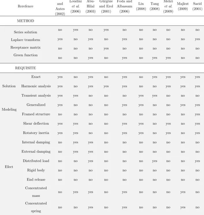
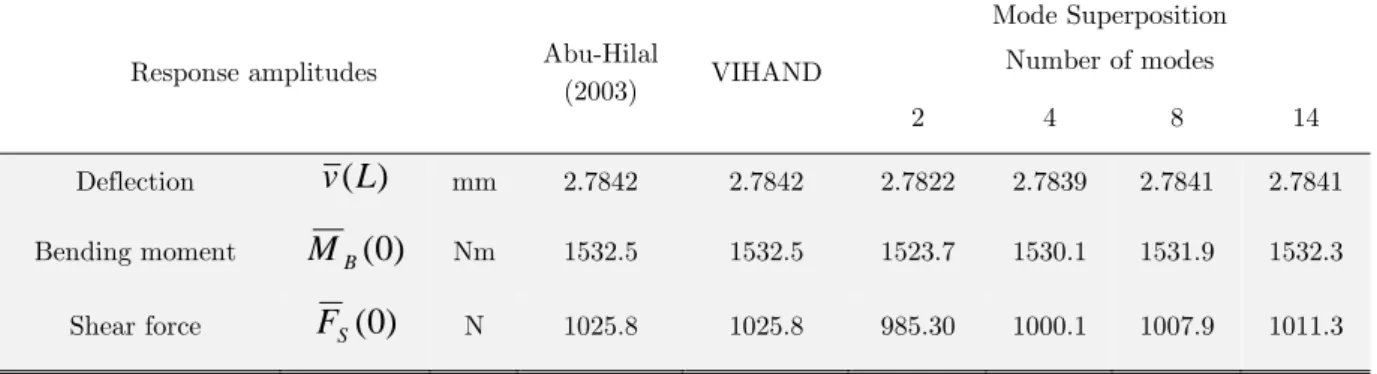
dedicated to dynamic frame response calculation do not conform to the requirements of an exact solution and therefore are not considered here. Concerning the dynamic response of frames, Table 1 compares different solution methods found in the literature [Abu-Hilal (2003), Foda and Albassam (2006), Gürgöze and Erol (2001), Lin (2008), Loudini et. al. (2006), Majukt (2009), Mehri et. al. (2009), Saeid (2011), Schanz and Antes (2002), Tang (2008)]. In the present context, it is imperative that the PDE representing the governing equations of a given in-plane structure subjected to harmonic forces has to be solved exactly. This can be achieved by using Laplace transform [Abu-Hilal (2003), Foda and Albassam (2006), Loudini et. al. (2006), Saeid (2011)] and/or Green functions [Abu-Hilal (2003), Tang (2008), Davar and Rahmani (2009)]. Gürgöze and Erol (2001) use a distinct method based on a receptance matrix but cannot be considered exact since series solution is employed.
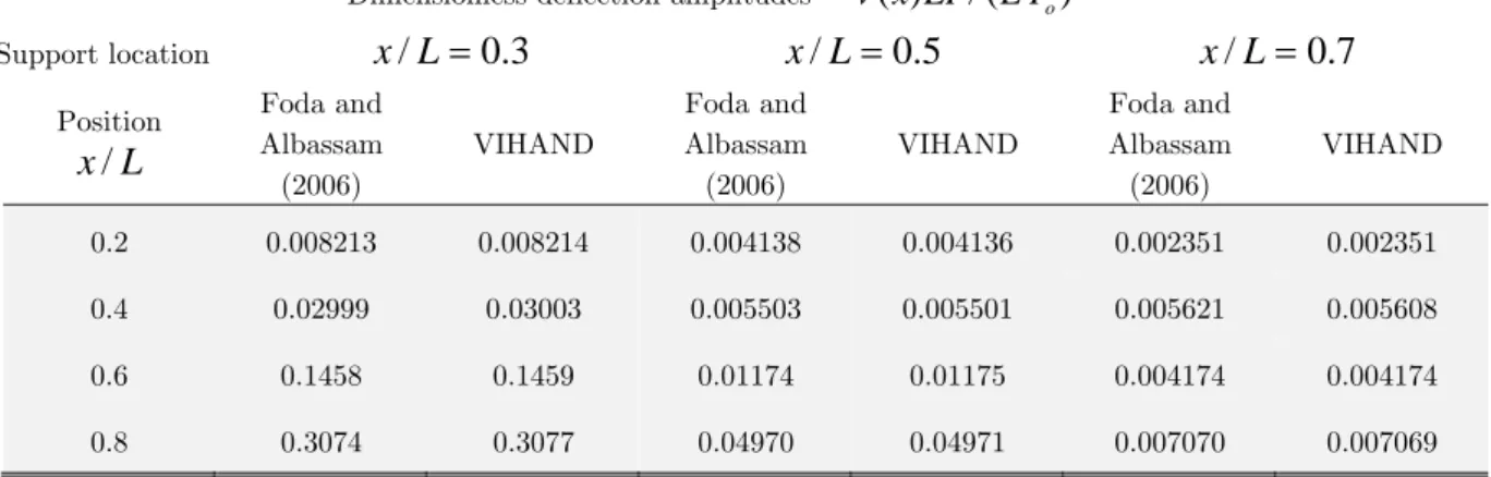
As seen in Table 1, only the solutions given in (Shanz and Antes, 2002; Foda and Albassam, 2006; Lin, 2008; Majkut, 2009; Saeid, 2001) could be generalized in order to solve models of arbitrary numbers of beams and boundary conditions. If further features are to be considered, e.g. concentrated masses and springs, these solutions would be limited to the ones developed in (Foda and Albassam, 2006; Majkut, 2009). Even so, these references are dedicated to solve single and/or in-line beams. When considering the capability to solve framed structures with the features of concentrated masses and springs and rigid bodies attached to the members ends, only Seeid (2001) can be highlighted. These features are not taken into account by Antes et al. (2004), which also deals with harmonic loads applied to Timoshenko frames. Mei (2008, 2012) present an interesting model that considers in-plane vibration of some restricted forms of frames. The analyses presented in these references are developed, as here, along the Timoshenko bending theory. In contrast, the present paper is more general inasmuch as it handles any shape of portal planar frame subjected to harmonic loads and it solves the equations of motion via the Laplace transform.
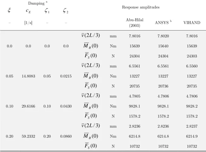
Except for the case of transient analysis, which is beyond the scope of this study, the solution of the present investigation is unique in the sense that attends to all of the requisites listed in Table 1. Indeed, to best of the author knowledge, no other publication in the context of harmonic analysis pays attention to effects like rigid offset and end release. Few publications (Abu-Hilal, 2003; Tang, 2008; Saeid, 2001) have considered distributed loads and even fewer have incorporated damping (Loudini, 2006; Abu-Hilal, 2003) in their analysis.
Rerefence
Schanz and Antes (2002)
Loudini
et al. (2006)
Abu-Hilal (2003)
Gürgöze and Erol (2001)
Foda and Albassam (2006)
Lin (2008)
Tang (2008)
Mehri
et al. (2009)
Majkut (2009)
Saeid (2001)
METHOD
Series solution Laplace transform Receptance matrix Green function
no yes no yes no no no no no no yes no yes no yes no no no no yes no no no yes no no no no no no no no yes no yes no yes yes no no REQUISITE
Solution
Exact yes no yes no yes no yes yes yes yes Harmonic analysis yes no yes yes yes no no yes yes yes Transient analysis yes yes no no no yes yes no no no
Modeling
Generalized yes no no no yes yes no no yes yes Framed structure no no no no no no no no no yes
Efect
Shear deflection yes yes no no yes yes no yes no yes Rotatory inertia yes yes no no yes yes no yes no yes Internal damping no yes yes no no no no no no no External damping no yes yes no no no no no no no Distributed load no no yes no no no yes no no yes Rigid body no no no no no no no no no no End release no no no no no no no no no no Concentrated
mass no yes yes no yes no no no yes no Concentrated
spring no no yes no yes no no no yes no
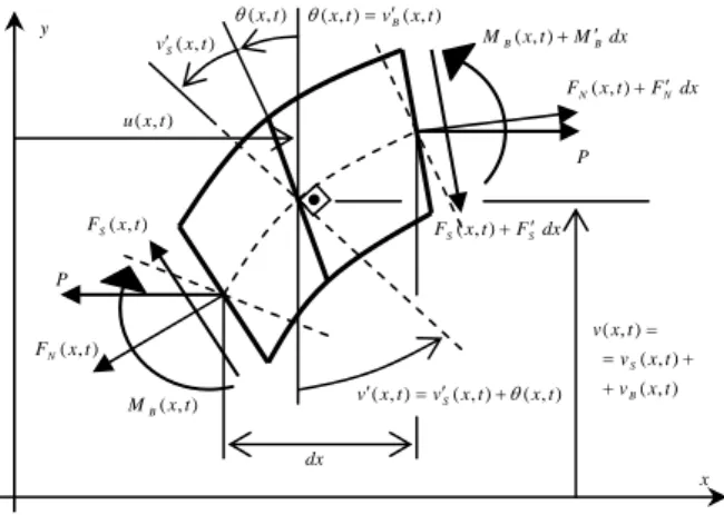
Figure 1: Timoshenko beam: internal forces and displacements at local coordinates.
Taking into account external and internal damping effects, Section 2 is dedicated to presenting the basic equilibrium equations of a flexible span, in both axial and transverse directions. For the transverse equilibrium, the Timoshenko beam theory (Howson and Williams, 1973; Dias and Alves, 2009; Schanz and Antes, 2002; Loudini et al., 2006) is applied in order to consider the effects of shear deflection and distributed rotatory inertia. In Section 2.2, under the assumption in Section 2.1 that all the excitations vary harmonically with the same frequency, the steady state response is formulated in terms of displacement and force amplitudes, which are then subjected to the Laplace transform. Although this assumption reduces the application scope, it characterizes the well-known harmonic analysis, useful to identify harmful vibrations due to resonance occurrences. On the other hand, considering that a given beam like structure is linear, the proposed method can be extended to a more general excitation type, with more than one distinct excitation frequency.
The first order governing equations of Section 2 are a coupled PDE system that might be manipulated in order to obtain uncoupled PDEs for the displacements (Howson and Williams, 1973; Foda and Albassam, 2006). However, this operation would produce fourth order PDEs that are less suitable for Laplace transform (Schanz and Antes, 2002). Hence, in Section 3, the equations of Section 2 are directly subjected to Laplace transforms such that, after some easier but laborious algebraic operations, decoupled results for displacements and forces could be obtained in the Laplace domain.
After applying inverse Laplace transforms to the results of Section 3, Section 4 gives the desirable formulations for the internal displacements and forces of the member flexible span, which are expanded to the model global matrices in Section 5. As it is shown there, from these formulations it is possible to obtain the relation between end forces and end displacements such that the member dynamic stiffness matrix and the member equivalent load vector can be defined. Then, using a similar technique to the finite element method, it is shown how these member matrices are employed to establish the global matrices that represent the dynamic equilibrium of the framed structure.
P
dx
) , (xt
) , (xt vS
dx F t x FN(,) N
P
dx F t x FS(,) S
dx M t x MB(,) B
) , (xt FN
) , (xt FS
) , (xt MB
x y
) , (
) , (
) , (
t x v
t x v
t x v
B S
) , ( ) , ( ) ,
(xt v xt xt v S
) , ( ) , (xt vB xt
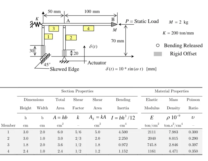
The solution of this equilibrium system directly gives the nodal displacements, from which easily follows member stresses. Some careful chosen examples in Section 6 illustrate the major features of the present method.
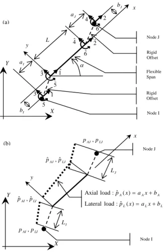
Figure 2: Member properties: (a) geometry and degrees of freedom (Dofs) in local coordinates:
6
,
,
2
,
1
Dofs at element nodes;1ˆ
,
2ˆ
,
,
6ˆ
Dofs at flexible span ends; (b) distributed axial and lateral loads2 BASIC EQUATIONS
According to the Timoshenko beam theory (Howson and Williams, 1973; Dias and Alves, 2009; Schanz and Antes, 2002; Loudini et al., 2006) and considering the internal forces and displacements in Fig. 1, with the distributed linear varying external forces in Fig. 2.b, the following equations are obtained, with the prime denoting the derivative wrt position,
x
, overdot denoting derivative wrt time,t
, and all the loads varying in time with the same circular frequency
:J b
y L
J a
I a
I b
x
1
2
3
4
5
6
1ˆ
2ˆ
3ˆ
4ˆ
5
6ˆ
Node I Node J
Flexible Span Rigid Offset
Rigid Offset
X Y
LJ AJ p pˆ ,ˆ
y
X Y
x
Node I Node J
LI AI p p ,
LI AI p pˆ ,ˆ
I L
J L LJ AJ p p ,
A A A x a x b pˆ ( ) :
load Axial
L L L x a x b pˆ ( ) :
load Lateral (a)
Normal stress, ʺN
( , ) [ ( , ) ( , )]
N x t E u x t c u x tI
s = ¢ + ¢ (1)
Normal force, FN
( , ) ( , ) [ ( , ) ( , )]
N N I
F x t =As x t =EA u x t¢ +c u x t¢ (2)
Axial equilibrium
t j A A E
N
x
t
m
u
x
t
mc
u
x
t
a
x
b
e
F
(
,
)
(
,
)
(
,
)
(
)
(3)Mean shear stress, ʻ
( , )x t G v x t [ ( , )S c vI S( , )]x t
t = - ¢ + ¢ (4)
Shear force, FS
( , )
( , )
( , )
[
( , )
( , )]
( , )
[ ( , )
( , )]
[ ( , )
( , )]
S S S S I S
S I S I
F x t
A
x t
Pv x t
GA v x t
c v x t
Pv x t
GA
x t
c
x t
GA v x t
c v v x t
(5)Transverse force equilibrium
t j L L E
S
x
t
m
v
x
t
mc
v
x
t
a
x
b
e
F
(
,
)
(
,
)
(
,
)
(
)
(6)Bending stress, ʺB
)
,
(
)
,
(
[
))]
,
(
)
,
(
[
)
,
,
(
x
y
t
yE
v
Bx
t
c
Iv
Bx
t
yE
x
t
c
Ix
t
B
(7)Bending moment, MB
( , ) ( , ) [ ( , ) ( , )]
B B I
M x t =
ò
ys x t dA =EI q¢x t +c q¢x t (8)Moment equilibrium
)
,
(
)
,
(
)
,
(
)
,
(
)
,
(
)
,
(
)
,
(
x
t
F
x
t
P
v
x
t
r
v
x
t
F
x
t
P
v
x
t
r
x
t
M
B
S
B
S
(9)In these equations, the internal and external damping coefficients,
c
I andc
E, respectively, are defined in order to reproduce the Rayleigh formulation, wherec
E represents the mass proportional coefficient andc
I the stiffness proportional coefficient. From this, by using the orthogonal condition of the natural modes, it is possible to establish the following expression for the modal damping ratio
i:2
/
)
/
(
E i I ii
c
c
(10)Meaningful values for
c
I andc
E can be obtained whenever a pair of modal damping ratio values is known. Therefore, after applying Eq. (10), these damping coefficients can be computed by:)
/(
)
(
2
122 2 1 2 2 1 2
1
E
c
(11.a))
/(
)
(
2
122 2 1 1 2
2
I
c
(11.b)where the natural frequencies (
1,
2) and the damping ratios (
1,
2), for the lowest first andsecond modes, are supposedly known.
On the other hand, by imposing that both Rayleigh damping coefficients must be non-negative and that the peak frequencies
pi given by:2
2
1
ii
pi
(12)must be real, the following restrictions must be obeyed:
)
/
(
)
/
(
1 2 2 1 2 11
(13.a)0.707
/2
2
,
21
(13.b)The external damping coefficient
c
E accounts for the environment viscous actions expressed by the forcesc
u
( t
x
,
)
andc
v
( t
x
,
)
, so that:1
[ ]
E
c c s
m
- = (14.a)
The internal damping coefficient
c
I accounts for the energy dissipation due to the structure deformation rate and can be related with the Kelvin-Voight damping coefficientK
V (Shanz and Antes, 2002):E
K
s
c
I[
]
V/
(14.b)2.1 Steady state response
For the steady state response, all the previous defined internal forces and displacements can be written according to the general equation
t j
e
x
F
t
x
F
(
,
)
(
)
(15)with time and space being decoupled.
Performing time derivatives in equations (1-9), the amplitudes are related by:
)
(
)
1
(
)
(
x
EA
jc
u
x
F
N
I
(16.a))
(
)
(
)
(
)
(
2 E A AN
x
m
jc
u
x
a
x
b
F
(16.b))
(
]
)
1
(
[
)
(
)
1
(
)
(
x
GA
jc
x
GA
jc
P
v
x
F
S
S
I
S
I
(16.c))
(
)
(
)
(
)
(
2 E L LS
x
m
jc
v
x
a
x
b
F
(16.d))
(
)
1
(
)
(
x
EI
jc
x
M
B
I
(16.e))
(
)
(
)
(
)
(
x
F
x
P
v
x
r
2x
M
B
S
(16.f)where, for instance, v x( ), is the amplitude of the beam total deflection.
2.2 Laplace Transform
Applying the Laplace transform over the previous defined amplitudes:
0
( ) [ ( )[( )] ( )sx
F s lF x s F x e dx ¥
= =
ò
(17)
the differential equations (16) are substituted by the following simple algebraic expressions:
)]
0
(
)
(
~
)[
1
(
)
(
~
u
s
u
s
jc
EA
s
F
N
I
(18.a)s
b
s
a
s
u
jc
m
F
s
F
s
~
N(
)
(
0
)
(
2
E
)
~
(
)
A/
2
A/
(18.b))]
0
(
)
(
~
][
)
1
(
[
)
(
~
)
1
(
)
(
~
v
s
v
s
P
jc
GA
s
jc
GA
s
F
S
S
I
S
I
(18.c)s
b
s
a
s
v
jc
m
F
s
F
s
S(
)
(
0
)
(
E)
~
(
)
L/
L/
~
2
2
(18.d)
)]
0
(
)
(
~
)[
1
(
)
(
~
EI
jc
s
s
s
M
B I (18.e))
(
~
)]
0
(
)
(
~
[
)
(
~
)
0
(
)
(
~
2s
r
v
s
v
s
P
s
F
M
s
M
s
B
B
S
(18.f)It is adopted in the sequence, according to Fig. 2.a, the convention for the end forces and end displacements as 1
ˆ
)
0
(
q
1
ˆ
)
0
(
p
F
N
F
S(
0
)
p
ˆ
3M
B(
0
)
p
ˆ
5 (19.b)Now, solving Eqs. (18.a) and (18.b) for the axial displacement results in:
1 20
(
)
~
)
(
~
n n n
s
A
s
e
s
u
(20)with
)
/(
1
)
(
~
2 20
s
s
AA
(21.a)1 1
q
ˆ
e
(21.b))]
1
(
/[
ˆ
1 I
o
p
EA
jc
e
(21.c))]
1
(
/[
1
b
AEA
jc
I
e
(21.d))]
1
(
/[
2
a
AEA
jc
I
e
(21.e)where
)
1
(
)
/
1
(
A
m
EA
jc
E
jc
I (22)Total deflection can be obtained after considerable algebraic manipulation of Eqs. (18.c–f), yielding:
3 20
(
)
~
)
(
~
n n n
s
L
s
a
s
v
(23)with
)
/(
)
/(
1
)
(
~
22 2 2 1 2
0
s
s
s
L
(24.a)3 3
q
ˆ
a
(24.b)1 3
5
2
[(
1
jc
I
)
q
ˆ
p
ˆ
/
GA
S]
/
a
(24.c))
/(
)
(
ˆ
)
/(
ˆ
)
/(
1 5 1 3 0 2 11
b
GA
p
EI
q
P
r
EI
a
L
S
(24.d))
/(
ˆ
)
/(
1 3 0 10
a
GA
p
EI
a
L
S
(24.e))
/(
1 01
b
EI
a
L
(24.f))
/(
1 02
a
EI
a
L
(24.g)when adopting
)]
1
(
/[
1
20
S I
w
P
GA
jc
/
1
1
(25.b)2 / 1 3 2 3 2 1 1 2
,
1
{[
h
h
4
h
h
]
/(
2
h
)}
(25.c)and
EI
h
3
1 (26.a)2 0
2
1
EI
(
1
jc
/
)
m
/
GA
P
r
h
E S
(26.b)2 0
2
(
1
jc
/
)
m
h
E (26.c)Analogously, solving Eqs. 16(c-f) for the shear force and bending rotation results in:
23
0 1 3
2 3
)
(
~
/
ˆ
/
/
)
(
~
n
n n L
L
s
b
s
p
s
a
s
L
s
a
s
F
(27)
2
3
0 1 3
2
3 2 3
)
(
~
]
ˆ
)
(
~
[
)]
1
(
/[
]
/
ˆ
/
/
[
)
(
~
n
n n
I S
L L
s
L
s
a
q
s
v
s
jc
GA
s
p
s
b
s
a
s
(28)
with
)]
1
(
/[
)
/
1
(
2
m
jc
Ew
GA
S
jc
I (29)The Laplace transform of the bending moment can be obtained by inserting Eq. (28) into Eq. (18.e). The bending moment amplitude,
M
B(x
)
, comes from Eq. (16.e) once the rotation amplitude,
(x
)
, has been obtained.A common practice in the specialized literature is to decouple Eqs. (16) in order to obtain a set of differential equations involving only one unknown function. For the Timoshenko theory, complicated terms involving fourth order derivatives will appear, so the use of the Laplace transform is troublesome. To avoid this, here the Laplace transform was directly applied to the coupled first order Eqs. (16) by applying the transform to second order coupled equations involving only deflection and rotation. As a remark, Schanz and Antes (2002) also avoids to work with fourth order derivatives.
3 INVERSE LAPLACE TRANSFORM
By applying the inverse transform to Eq. (20) for the axial displacement and then using the result in Eq. (16.a) for the normal force, these corresponding amplitudes are then given, respectively, by:
1 2)
(
)
(
nn n
A
x
e
x
12 1 1
2
)
(
)
1
(
)
(
)
1
(
)
(
n
n n E
n n n E
N
x
EA
jc
e
A
x
EA
jc
e
A
x
F
(31)where, knowing that
)
(
)
(
x
A
1x
A
n
n
forn
0
(32.a)and
x nn
x
A
d
A
0
1
(
)
)
(
forn
0
(32.b)it holds that
1. For
n
0
,
2
,
4
,
6
...
)
(
)
1
(
)
(
x
/2 1sin
x
A
n
n
An
A (33.a)2. For
n
1
,
3
,
4
,
5
...
)
cos(
)
1
(
)
(
x
(1 )/2 1x
A
An A n
n
(33.b)3. For
n
2
,
4
,
6
,
( 2)/2
/2 1 2 1 2
0
( ) ( 1) [ sin( ) ( 1) / (2 1)!]
n
n n k k n k
n A A A
k
A x b b x x b k
- +
- + +
=
= - -
å
- + (33.c)4. For
n
1
,
3
,
4
,
( 1)/2
(1 )/2 1 2 2 1
0
( ) ( 1) [ cos( ) ( 1) / 2 !]
n
n n k k n k
n A A A
k
A x b b x x b k
- +
- - +
-=
= - -
å
- (33.d)As for the total deflection, it can be obtained by applying the inverse transform to Eq. (23), yielding
3 2)
(
)
(
nn n
L
x
a
x
v
(34)where
)
(
)
(
x
L
1x
L
n
n
forn
0
(35.a)and
x nn
x
L
d
L
0
1
(
)
)
with
1. For
n
0
,
2
,
4
,
6
,
]
/[
)]
(
)
(
[
)
(
222 1 2 1 2 1 1
1
sinh
x
sinh
x
x
L
n n n (36.a)2. For
n
1
,
3
,
5
,
7
,
]
/[
)]
cosh(
)
cosh(
[
)
(
x
11
1x
21
2x
12
22L
n n n (36.b)3. For
n
2
,
4
,
6
,
]
/[
}
)!
1
2
/(
)
(
)
(
)
(
{
)
(
2 2 2 1 2 / ) 2 ( 0 2 2 2 1 ) 1 2 ( 2 1 2 1 1 1
n k k n k n k n n nk
x
x
sinh
x
sinh
x
L
(36.c)4. For
n
1
,
3
,
5
,
]
/[
}
!
2
/
)
(
)
cosh(
)
cosh(
{
)
(
2 2 2 1 2 / ) 1 ( 0 1 2 2 1 2 1 2 2 1 2 1 1 1
n k k n k n k n n nk
x
x
x
x
L
(36.d)The rotation due to bending is obtained by substituting Eq. (23) into Eq. (28) and applying the inverse transform so that the amplitude is:
4 3 23
/
2
)
/[
(
1
)]
(
)
ˆ
(
)
(
n n n I S LL
x
b
x
GA
jc
b
L
x
a
p
x
forn
0
(37)With
3 2
4
q
ˆ
b
(38,a)1 2
3
a
b
(38.b)1 2 3
2
q
ˆ
a
b
(38.c)0 2 2
1
a
a
b
(38.d)1 2 1
0
a
a
b
(38.e)2 2 0
1
a
a
b
(38.f)1
2
a
b
(38.g)2
3
a
b
(38.h)and
)]
1
(
/[
1
2
Finally, the shear force amplitudes come from the inverse transform of Eq. (27), resulting in
2 3 1 2 23
/
2
(
1
/
)
(
)
ˆ
)
(
n n n E L LS
x
p
a
x
b
x
m
jc
w
a
L
x
F
(40)while the bending moment amplitude comes from the use of Eq. (37) in expression (16.e),
4 31
(
)
)
1
(
)
/(
)
(
)
(
)
1
(
)
(
n n n I S L L I Bx
L
b
jc
EI
GA
b
x
a
EI
x
w
jc
EI
x
M
(41)4 MEMBER MATRICES
4.1 Flexible span equilibrium
Applying the following boundary conditions for the end displacement (see Fig. 2.a):
2
ˆ
)
(
L
q
u
v
(
L
)
q
ˆ
4
(
L
)
q
ˆ
6 (42)after laborious algebraic work, the equations of the previous section can be rearranged in the following expressions for the internal displacements:
)
(
ˆ
)
(
ˆ
)
(
)
(
x
U
1x
q
1U
1x
p
1U
x
u
q
p
o (43.a))
(
ˆ
)
(
ˆ
)
(
ˆ
)
(
ˆ
)
(
)
(
x
V
3x
q
3V
5x
q
5V
3x
p
3V
5x
p
5V
x
v
q
q
p
p
o (43.b))
(
ˆ
)
(
ˆ
)
(
ˆ
)
(
ˆ
)
(
)
(
x
q3x
q
3
q5x
q
5
p3x
p
3
p5x
p
5
ox
(43.c)with the functions on the right hand sides (from
U
q1(
x
)
to
o(x
)
) being defined in Appendix A. Analogously, applying the following boundary conditions for the end forces:2
ˆ
)
(
L
p
F
N
F
S(
L
)
p
4M
B(
L
)
p
ˆ
6 (44)the internal forces are given by:
)
(
ˆ
)
(
ˆ
)
(
)
(
x
N
1x
q
1N
1x
p
1N
x
F
N
q
p
o (45.a))
(
ˆ
)
(
ˆ
)
(
ˆ
)
(
ˆ
)
(
)
(
x
S
3x
q
3S
5x
q
5S
3x
p
3S
5x
p
5S
x
F
S
q
q
p
p
o (45.b))
(
ˆ
)
(
ˆ
)
(
ˆ
)
(
ˆ
)
(
)
(
x
B
3x
q
3B
5x
q
5B
3x
p
3B
5x
p
5B
x
M
B
q
q
p
p
o (45.c)with the functions on the right hand sides (from
N
q1(
x
)
toB
o(x
)
) being defined in Appendix A. Now, defining the vectors:T A
{
q
ˆ
q
ˆ
}
ˆ
2 1
and
T A
{
p
ˆ
p
ˆ
}
ˆ
2 1
P
(47)and using the previous equations (43.a) for the axial displacement and (45.a) for the normal force, the axial equilibrium is expressed by:
0
φ
P
φ
Q
φ
QAˆ
A
PAˆ
A
OA
(48)with
0
)
(
1
)
(
1 1L
N
L
U
q q QA
φ
(49.a)
1
)
(
0
)
(
1 1L
N
L
U
p p PA
φ
(49.b)
)
(
)
(
L
N
L
U
o o OA
φ
(49.c)Equation (48), after multiplication by the inverse of
φ
PA, gives the following classical matrix equilibrium equation:A DA EA
A
P
K
Q
P
ˆ
ˆ
ˆ
ˆ
(50)with the vector of equivalent axial loads being
OA PA
EA
φ
φ
P
ˆ
1 (51)while the axial dynamic stiffness matrix is
QA PA
DA
φ
φ
K
ˆ
1 (52)Analogously, transverse equilibrium can be written as
L DL EL
L
P
K
Q
P
ˆ
ˆ
ˆ
ˆ
(53)with the equivalent lateral load vector and the dynamic stiffness matrix given by, respectively,
OL PL
EL
φ
φ
P
ˆ
1 (54)QL PL
DL
φ
φ
K
ˆ
1 (55)T L
{
q
ˆ
q
ˆ
q
ˆ
q
ˆ
}
ˆ
6 5 4 3
Q
(56) T L{
p
ˆ
p
ˆ
p
ˆ
p
ˆ
}
ˆ
6 5 4 3
P
(57)
0
)
(
0
)
(
0
)
(
0
)
(
1
)
(
0
)
(
0
)
(
1
)
(
5 3 5 3 5 3 5 3L
S
L
S
L
B
L
B
L
L
L
V
L
V
q q q q q q q q QL
φ
(58.a)
0
)
(
1
)
(
1
)
(
0
)
(
0
)
(
0
)
(
0
)
(
0
)
(
5 3 5 3 5 3 5 3L
S
L
S
L
B
L
B
L
L
L
V
L
V
p p p p p p p p PL
φ
(58.b)
)
(
)
(
)
(
)
(
L
S
L
B
L
L
V
o o o o OL
φ
(58.c)Now, combining both axial and lateral matrix equilibrium equations, it follows that:
Q
K
P
P
ˆ
ˆ
E
ˆ
Dˆ
(59)with the end displacements and end forces vectors being given, respectively, by
T
q
q
q
q
q
q
ˆ
ˆ
ˆ
ˆ
ˆ
ˆ
}
{
ˆ
6 5 4 3 2 1
Q
(60) Tp
p
p
p
p
p
ˆ
ˆ
ˆ
ˆ
ˆ
ˆ
}
{
ˆ
6 5 4 3 2 1
P
(61)The equivalent load vector is
EL EA EP
P
P
ˆ
ˆ
ˆ
(62)and the dynamic stiffness matrix is
4.2 Rigid offset
Observing Fig. 2, the conversions from the flexible span ends to the member ends are given by:
Q
T
Q
Qˆ
(64)Q
S
P
P
T
P
Qˆ
R
2 Qˆ
(65)where
1
0
0
0
0
0
0
1
0
0
0
0
0
1
0
0
0
0
0
1
0
0
0
0
0
1
0
0
0
0
0
1
J I J I Qa
a
b
b
T
(66.a)
3
/
ˆ
6
/
3
/
ˆ
6
/
2
/
)
ˆ
(
2
/
)
ˆ
(
2
/
)
ˆ
(
2
/
)
ˆ
(
0
0
0
0
0
0
0
0
0
0
0
0
0
0
0
0
0
0
0
0
0
0
0
0
0
0
2 2 LJ LJ LI LI LJ LJ AJ AJ LI LI AI AI J I J J I I J J I I Rp
p
p
p
p
p
p
p
p
p
p
p
L
L
a
b
a
b
b
a
b
a
P
(66.b)
1
0
0
0
0
1
0
0
0
0
1
0
0
0
0
0
0
1
0
0
0
0
0
0
1
0
0
0
0
0
0
1
J J I I Pa
b
a
b
T
(66.c)]
[
T
I
HJU
S
Q
Q
(66.d)with
]
[
diag
M
TIM
TIM
RIM
TJM
TJM
RJ
J
(67.a)
1
0
0
0
0
0
0
0
1
0
0
0
0
0
0
0
1
0
0
1
0
0
0
0
0
0
0
1
0
0
0
0
0
0
0
1
5
.
0
U
(67.b)
1
2
/
2
/
0
0
0
0
0
0
1
2
/
2
/
0
1
0
0
0
0
0
0
0
0
1
0
0
0
1
0
0
0
0
0
0
0
0
1
J J I Ia
b
a
b
H
(67.c) AI AI AJ T IAI
L
L
p
p
p
p
ˆ
(
)(
)
(67.d)LI LI LJ T I
LI
L
L
p
p
p
p
ˆ
(
)(
)
(67.e)AI AI AJ T I
AJ
L
L
L
p
p
p
p
ˆ
[(
)
/
](
)
(67.f)LI LI LJ T I
LJ
L
L
L
p
p
p
p
ˆ
[(
)
/
](
)
(67.g)2 2
I I
I
a
b
L
(67.h)2 2
J J
J
a
b
L
(67.i)J I
T
L
L
L
L
(67.j)Now, collecting
P
ˆ
andQ
ˆ
from expressions (64, 65) and substituting into Eq. (59), member equilibrium requires that:Q
K
P
P
E
D (68)where, for the member equivalent load vector and the member dynamic stiffness matrix, respectively, we have:
R E P
E
T
P
P
P
ˆ
(69)1 2
)
ˆ
(
P D Q QD
![Figure 3: Frequency response for the simply supported Timoshenko beam of Table 6 with two symmetrically attached springs: (a) deflection at load location [mm]; (b) bending moment at load location [Nm]](https://thumb-eu.123doks.com/thumbv2/123dok_br/18885063.423630/26.808.240.687.157.662/frequency-response-supported-timoshenko-symmetrically-attached-deflection-location.webp)
![Figure 5: Frequency response for the elastic robot manipulator of Fig. 4: (a) deflection [mm] at point B;](https://thumb-eu.123doks.com/thumbv2/123dok_br/18885063.423630/28.808.169.677.250.895/figure-frequency-response-elastic-robot-manipulator-deflection-point.webp)
