A Work Project, presented as part of the requirements for the Award of a
Master’s Degree in Finance from the NOVA – School of Business and Economics
and a
Professional Master in Finance from the
Fundação Getúlio Vargas - São Paulo School of Economics.
Carbon Markets Efficiency
An empirical study on the key price determinants of the EU
ETS from 2009 to 2016
José Júlio Valente da Silva Gonçalves FGV-EESP Student Number: 334848
Nova SBE Student Number: 2509
Project carried out on the International Master in Finance Brazil-Europe course, under the supervision of:
Professor Marcelo Fernandes (EESP-FGV, São Paulo, Brazil) Professor João Pedro Pereira (Nova SBE, Lisbon, Portugal)
ACKNOWLEDGEMENTS
First and foremost, I would like to express my sincere gratitude and special appreciation to my supervisors, Professor João Pedro Pereira at NOVA SBE and Marcelo Fernandes at EESP-FGV, for their encouragement and insightful guidance throughout the Work Project.
I would also like to express gratitude to the staff and my colleagues from the IMF program and the extensive facilities of both institutions. It was a pleasure to be part of such a demanding, scientific rigorous and life changing program, which I highly recommend to future applicants.
ABSTRACT
This work project is an empirical study on the key price driven factors of the European Union Emissions Trading Scheme. The research examines the prices on the secondary market, from 2009 until 2016, comprehending the second and third phases of the program, performed with an Ordinary Least Squares regression. The independent variables under the scope of this project are not only energy based, but also structured spreads, economic growth proxies and a temperature dispersion indices.
First, the results are due to respect of the whole period to present a global picture of the main determinants on the carbon price changes then, the sample is divided according with institutional measures to avoid over allocation and price instability.
Evidence suggests the impact of energy-related variables such as Brent, Coal and the Power Price in Germany and in the U.K. on the price of European Union Allowances, especially during the 3rd phase of the scheme. Moreover, fluctuations in the coefficients and in the explanatory variables are highly related with institutional changes on the European program.
LIST OF FIGURES
1 – Explanation of the cap-and-trade system. Source: The Government of Quebec. 2 – Emissions trading timeline.
3 – Emissions in 2015 by Sector. Source: Reuters Point Carbon.
4 – Short and long positions by country and sector. Source: Kettner et al. (2006). 5 – EUA Spot Price. Line & Symbol Eviews’ graph.
6 –EUA 1st logarithm difference. Line & Symbol Eviews’ graph. 7 – Month-ahead energy prices. Line & Symbol Eviews’ graph. 8 – OLS residuals, actual and fitted generated by Eviews. 9 – Recursive residuals tests generated by Eviews. 10 –Eviews’s CUSUM test.
11 – CUSUM of Squares test generated by Eviews.
LIST OF TABLES
1 – Global Warming Potential Index. Source: Intergovernmental Panel on Climate Change. 2 – Normality test of the 1st Logarithm difference of the EUA.
3 – Correlation Matrix, generated by Eviews. 4 – Descriptive statistics, generated by Eviews.
5 – OLS regression for the whole period and accounting with all dependent variables. 6 – Adjusted OLS regression for the whole period.
7 – Adjusted OLS regression for the 2nd phase of the EU ETS. 8 – Adjusted OLS regression from 2009 until May 2011. 9 – Adjusted OLS regression for the third phase.
10 – Adjusted OLS regression for the 3rd phase, 1st year. 11 – Adjusted OLS regression for the 2nd year of the 3rd phase. 12 – Adjusted OLS regression for the 3rd phase, 2015.
13 – Adjusted OLS regression for current year of the 3rd phase. 14 - Normality test of the OLS residuals.
15 – Breusch-Godfrey Serial Correlation LM Test. 16 – Breusch-Pagan-Godfrey Heteroskedacity Test. 17 – Heteroskedasticity Test: White test.
18 – Ramsey RESET Test.
TABLE OF CONTENTS
1. Introduction ... 6
2. Terminology ... 7
3. Emissions Trading ... 10
4. EU ETS ... 12
5. Price Driven Factors ... 18
5.1 Supply Determinants ... 19
5.2 Demand Determinants ... 21
6. Research Question ... 23
7. Empirical Methodology ... 24
8. Data ... 30
9. Results ... 31
9.1 OLS: 2009-2016... 35
9.2 OLS: second phase, 2009 – 2013 ... 36
9.3 OLS: third phase, 2013 – 2016 ... 37
9.4 OLS: third phase, year by year... 38
9.5 Robustness ... 41
10. Conclusion ... 45
REFERENCES ... 47
1.
Introduction
As one of the most recent trends, emissions trading is currently facing a period of unparalleled development all over the globe, alongside with new investment products copulated with a green label that are prompt to take over the global markets sooner than expected.
Emissions Trading Scheme, a fairly new trading platform available on several countries around the globe, is expected to be one of the main contributors to limit global warming up to 2ºC1, as agreed in one of the most recent climate conferences in Paris 2015. However, several questions have been raised on how efficient carbon markets currently are and what is driving price changes.
To access how efficient is a scheme and, therefore, how likely it is to contribute to the abatement of emissions, I will perform an empirical model with the main goal to explain price movements of the European Carbon Price. I will evaluate the significance of external determinants, such as energy prices or macroeconomic environment and, at some extend, the impact of institutional changes on the spot price, throughout a 7-years period.
My results show empirical evidence of the impact of institutional changes on the European Union Allowance Spot price and the main key determinants, especially for the 3rd phase of the scheme.
2.
Terminology
Greenhouse gases (GHG) is used as a reference when describing gases that are trapped in the atmosphere. According with EPA2, in 2014 Carbon Dioxide (CO) was responsible for 81% of the total GHG emissions in the U.S. The other relevant gases are Methane (CH4)
11%, Nitrous Oxide (6%) and Fluorinated Gases (3%). Table 1, in the appendix, describes the level of global warming with CO2 as indicator3. As it is possible to observe, 1kg of CH4
causes 25 times more warming over a 100 year period than the same amount of CO2,
meaning that even if it is present in a smaller percentage, CH4 is highly prejudicial.
An Emission Trading Scheme (ETS) is a policy instrument for managing GHG emissions4. It was simply described in a British newspaper article as an upper limit on the total amount of GHG emissions allowed for emitters within the ETS jurisdiction. Entities are obliged to measure and report their carbon emissions, while they are allowed to trade excesses.5
To do so, emitters acquire an Emission Allowance (EA), which was formal defined by the European Union Emissions Trading Scheme6 (EU ETS) as a permit to emit one ton of CO
equivalent during a specific period, which shall be transferable, therefore, tradable. The term has been extended to cover the other GHG throughout the years.
2www.epa.gov
3www.ipcc.ch/ 4www.ieta.org
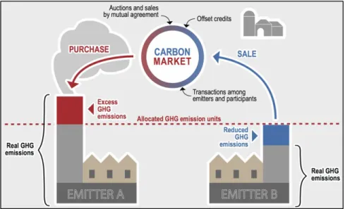
The Cap-and-Trade (CAT) strategy is a mechanism that sets an absolute limit on the total emissions while allows EAs to be traded among other covered entities. A common opposite example of this strategy is a Baseline-and-Credit system that defines a cap, such as relative target, only allowing emission reductions that go beyond it to be used as sellable credits, commonly described as an offset mechanism. ETS is used a reference for both these systems.
Fig. 1 -The cap-and-trade system. Source: The Government of Quebec.
The political feasibility of each scheme cannot be excluded from the discussion table since it is highly related to not only to the requirements for participation and consensus, but also to the transaction costs. As, in every scheme, players need to agree on a common regulatory framework, this is one of the most crucial aspects of my research as it institutional changes have a direct impact on the carbon price.
determinant blocking point in the creation of a climate policy, preventing high levels of participation in integrated trading schemes and, ultimately, the integration of multiple schemes into one unique framework. This is especially true when looking into the Western Climate Initiative, on which we observe a constant in-and-out flow of participants.
Dark spread is a measure used to evaluate the returns over fuel costs of coal-fired power plants.7 It accounts with the power price ($/MWh) and the fuel costs, including both the cost of the fuel ($/MMBtu) and the transportation costs ($/MMBtu), the calorific value (MMBtu/ton) and the heat rate (MMBtu/MWh). Like the dark spread, the spark spread measures the returns from selling a unit of electricity over a gas-fired plant, take into consideration the power price, gas price and heat rate.
Clean Dark and Spark spreads were introduced as an adjustment to the original metrics described above. Both consider the indicative prices of emissions8, with the purpose to evaluate changes in production costs of electricity generation and the economic incentives in shifting to a less GHG heavy-based fuel9.
When an enterprise issue stocks or bonds for the first time and sell them directly to investors, those transactions take place on the primary market. Furthermore, any other transaction on the same assets is done on the secondary market. Both primary and secondary markets concepts are also applied to emissions trading and will described in more detail in section 4.
7www.eia.gov/todayinenergy/detail.php?id=10051
3.
Emissions Trading
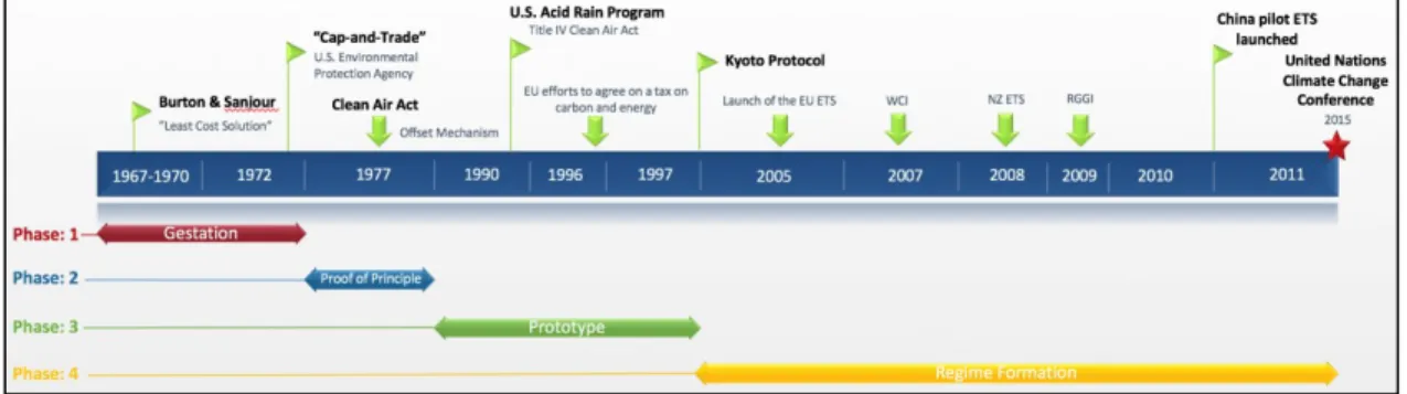
As part of a global effort to decrease of GHG emissions, the Kyoto Protocol signed in December 1997 was a major step in the recognition of the theoretical benefits of allowing emission reductions to be obtained at least cost through an international trading system of allowances. However, unlikely as it is wrongly refer to, the emission trading’s roots were not introduced in Kyoto but by a pioneer American system back in 1972.
A computer-based system was used to compare the cost and effectiveness of various multiple strategies (Burton And Sanjour, 1967). With access to several American cities emissions data, each strategy was compared with the least costly combination to achieve a specific abatement level, a common procedure in multiple environment related experiences. In 1972, after several improvements on these computer-assisted models, the newly created U.S. Environmental Protection Agency (EPA) introduced in its annual report the concept of CAT.
After the Gestation phase, the second stage took off with the Proof of Principle and the Clean Air Act in 197710, two of the most important marks in emissions trading history. The Clean Air Act consisted in an offset-mechanism where a company would be able to buy allowances from the Act after negotiate with another peer a decrease in the same degree, a similar mechanism is used today.
In the first 15 years of the Amendments became law (1972-1987), intensive polluters industries faced several losses in their income due to the newly abatement ruling (Greenstone, 2001). Even if losses were substantial, they were modest when compared to the size of the entire manufacturing sector, which suggested that new regulation implemented deterred the growth of polluters, which contradicts the overall aim of the program, the reduction of air pollution yet, never at the expenses of a specific sector.
Moreover, the U.S. Acid Rain Program introduced in the 1990 Clean Air Act11, part of the third stage, aimed to reduce the Sulfur Dioxide (SO) emissions of electricity and was the world’s first large-scale implementation of such a program, introducing a banking behavior in which pollution allowances could be used or stored, and buyers were able to resell them after, one of the features observed in today’s schemes. The European Union also undertook an ambitious effort to provide a carbon price signaling thanks to the introduction of an European tax on energy and carbon in the early 90’s. Eventually, this effort would fail since an unanimous agreement between all member states was required but, unfortunately, not achieved. Nevertheless, the standpoints for the Kyoto Protocol were launched for what would be the revolution of emissions trading.
After the 1997 meeting, an agreement to reduce GHG emissions through different mechanisms was reached. Emissions trading schemes were part of the solution and started to be planned and developed by different regions all over the globe ever since. The Protocol
was considered a landmark in environmental protection especially due to the collaboration of multiple nations, even without the ratification of the U.S.
The next figure summarizes the emissions trading history described until the Paris Agreement ratified in 2015.
Fig. 2 – Emissions trading timeline.
The implications of the Paris’ Agreement will not be taken into detail. Regardless, it was a clear breakthrough to reduce GHG emissions and further necessary considerations regarding its mandates will be duly pointed out.
4.
EU ETS
program, while mentioning impactful institutional changes among the other trading schemes that should be taken into account for future research purposes.
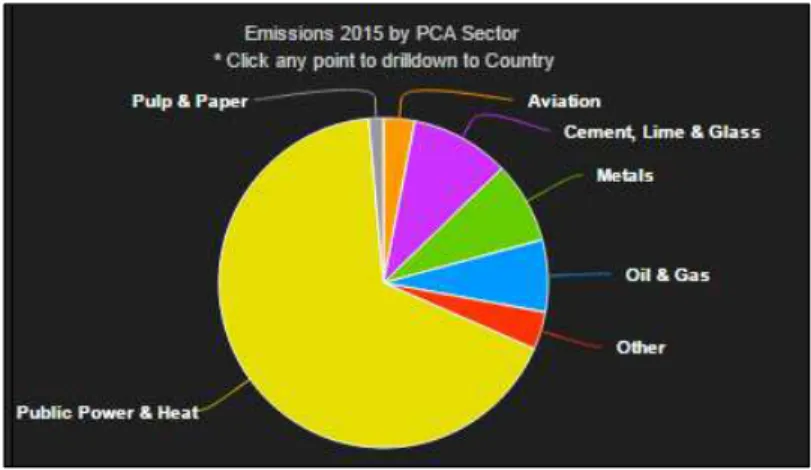
The EU ETS was the first large-scale GHG trading program, launched back in 2005, being since then widely known as the more developed scheme in the emissions trading scope. It currently covers more than 11,000 energy-using installations within 3 major industrial sectors, such as power and heat stations, over 31 countries12. On the other hand, one of its American peers, the Regional Greenhouse Gas Initiative (RGGI) only covers 9 United States, representing a total of about 23% of the GHG emissions13, while the Western Climate Initiative faced multiple changes in its affiliates during the years and, consequently, the total covered range has been adjusted since the start of the program.
Figure 3 shows the main sectors which contribute the most for GHG emissions in the Eurozone. Public power and heat sectors account for more than half of the 2015 emissions in Europe and Germany was responsible for about 25% of them followed closely by the U.K. and Poland as the main emitters. The weight and relevance of those countries is also applied for other sectors such as metals or oil and gas and it is the main reason for both Germany and the U.K. figures are the proxies used in some variables, in order to capture the main emitters inside the EU ETS and to analyze power prices and related spreads. For future developments, I would suggest to also include Poland’s prices as a proxy for the EU energy market and heavier GHG emitters.
12www.ec.europa.eu
Fig. 3 – Emissions in 2015 by Sector. Source: Reuters Point Carbon.
The European scheme is mandatory for all the 28 EU member states, with the additional participation of Norway, Iceland and Liechtenstein, covering approximately 45% of the total EU’s GHG emissions, targeting 57% of the 2005 level by 2030, far more than any other scheme in place at the moment. The goal however, is to increase the total percentage year by year with the addition of new facilities or sectors.
Working under the CAT principle, the EU sets a threshold to limit GHG emissions and then, distributes or sells European Union Allowances (EUA). The total amount of permits is reduced over time and companies, which emitted less than the correspondent EUA acquired, can sell the excess to other facilities.14 There is no price floor, opposite to the 2$ mark set by the RGGI in 2012, which increases annually at a rate of 2.5%. Another remarkable different mechanism in place is the New Zealand ETS, which sets a price ceiling of 25$ to avoid constrains for local facilities that compete overseas15, alongside being the only scheme not working with the CAT mechanism. The scheme uses an intensity-based system which allows enterprises to charge the final client for the emission
cost, rather similar to a carbon tax. With great results so far in decreasing the GHG emissions, the success of this approach is being currently studied by other countries and schemes as an alternative to the CAT traditional approach.
Domestic and international offsets are possible until the end of the 3rd phase, meaning a company can invest in a project that lower GHG emissions, such as forestry, creating an offset credit that can be either used or sold, typically at a lower price than purchased.16 Borrowing is possible within the trading period but not between stages, while banking is unlimited. Trading is also possible on Over-The-Counter (OTC) markets and organized exchanges. As it will be explained later, the secondary market will be the one captured by the dependent variable of my empirical model. There are multiple exchanges offering EU ETS Allowances derivative products such as the European Energy Exchange (EEX) or the European Climate Exchange (ECX), futures contracts for example, traded at the ICE and other exchanges, which are more liquid, thus highly appreciated for hedging or speculation purposes.
Due to the price turmoil of the first two stages, a considerable shift in the EAs allocation strategy was taken to surpass the pricing mechanism established before. The first phase lasted until 2007, as a “learning by doing” trading period, characterized by an excessive number of EAs, freely distributed, resulting in a price sunk. Similar behaviors were observed in other schemes all around the globe, however on a much lower scale than the
EU ETS, as they had the time to readjust the scheme accordingly with the European backlash.
Currently, auctions of EUAs are hold by the EEX and ICE, depending on which country are the EUAs attributed to. Nevertheless, the most common auction is hold for the whole EU by the EEX. Purchasing one contract entitles one EUA, which accounts for 1 ton of CO2
equivalent. The tick size is 0.01€ per allowance and the delivery day is one day after the
auction. For the sake of clarity, the primary market is a reference for these auctions, i.e., whenever a new EUA is launched.17 Secondary markets are available in emissions trading, specifically for the EUAs. In fact, due to daily quote availability, the secondary market will be the one under study, more precisely the one offered by EEX since 2005. I will consider EUA prices, meaning I will not include the aviation sector, due to its recent inclusion in the EU ETS scope and the fact they are traded separately.
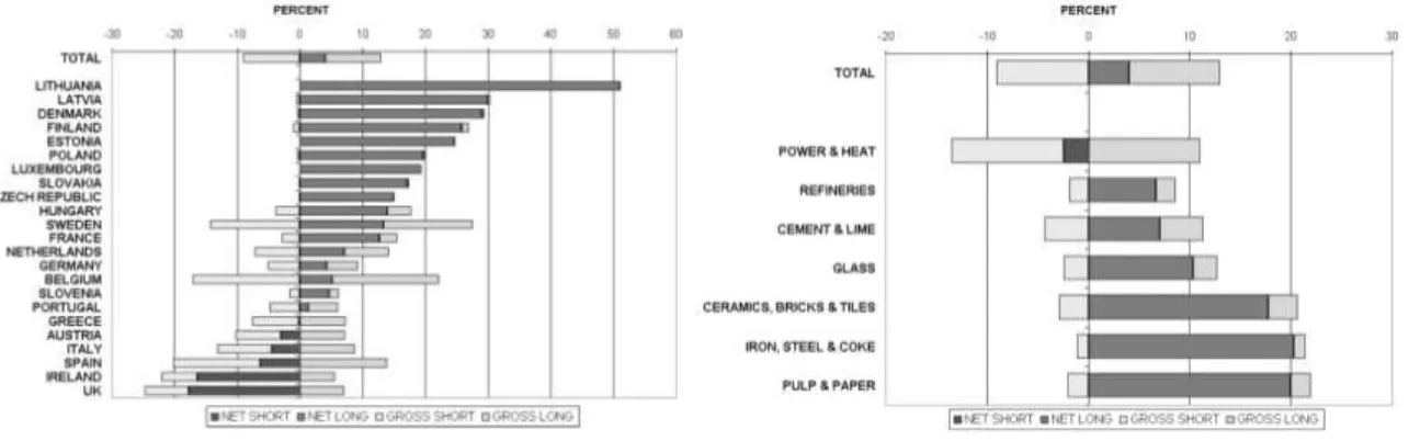
Seen as a case study in what could go wrong and, as previously highlighted, EU legislators were not careful enough in setting the initial cap, letting companies to easily achieve their targets and permit prices quickly depreciated. Hintermann (2009) underlines the additional influence on the price volatility due to special weather conditions such as high summer temperatures and low precipitation. To confirm his claim, I use a proxy for temperature dispersions, which will allow me to either refute or accept his findings. Alongside, over-allocation started to became an issue, not only per country but also per sector (Neuhoff,
Karsten et al., 2006), setting even more pressure on the EU to readjust the scheme accordingly to avoid more price turbulence.
Fig. 4 - Short and long positions by country and sector. Source: Kettner et al. (2006).
The electricity sector was short, while non-electricity industrial sectors were long. At the same time, a net short position is clearly seen among the EU15 member states has the major preference, while the vast majority of the new EU10 members, e.g., Lithuania and Latvia, were long.
During the second phase, free allocation represented about 92% of the total Cap18, while on the current stage it only accounts for about 43%, being auctions the main mechanism used to guarantee carbon permits. To achieve this, the regulators decreased by 6.5% the total number of EAs. However, once the global financial crisis hit, the economic downturn resulted in the cut of GHG emissions and thus demand. Carbon prices sunk once again yet showing a more stable pattern.
New Entrants Reserves (NER) are up to 5%, allowing for new participants in the scheme and cost containment and price support measures will be heavily supported in 2019, thanks
to a Market Stability Reserve19 (MRS), a long-term solution with a special focus on providing indirect pricing support by removing surplus allowances. On contrast, the New Zealand ETS leaves no room for new entrants within each compliance period. Back-loading was introduced in the 3rd phase to postpone the auctioning off 900M allowances from 2014-2016 until 2019/2020, and is expected to rebalance the supply and demand equilibrium, reducing carbon pricing volatility. A linear reduction factor was applied to the decrease the overall cap by 1.74%, from 2008 until the beginning of the 3rd phase, eventually reaching 2.2% by 2030 accordingly within the climate and energy policy framework representing, on average, almost 2.0% per year, from 2013 until 2020, without accounting with commercial aviation. Such amendments have been proven to be highly impactful on the EUA price, especially on the primary market. However, they are phased, i.e., impossible to quantify their impact on daily data. As so, even if they are not included directly in my empirical model, they will be considered by splitting the sample per period accordingly.
As previously pointed out, the EU ETS is, without a doubt, a starting point on which other schemes proceeded to learn not only from its main accomplishments in the abatement of GHG emission, but also by its adjustments and continuous refurbishing. For future research, other significant scheme related aspects should be taken into account.
5.
Price Driven Factors
The usage of Carbon Allowances is a function of the expected emissions per emitter. As so, the level of emissions depends on several factors such as fluctuations in energy
consumptions and production, traditional energy-based prices like coal, oil, etc., extreme weather conditions and finally, economic power. On the other hand, carbon prices are also determined by institutional decisions as mentioned. For example the amount available for emitters and further banking or borrowing limitations, new entrants reserves or price support measures, will have a direct effect on the auctioning price practiced.
Ellerman and Buchner (2007) argued the carbon price during the first stages of the European Scheme was mainly determined by allowances allocation issues – auctioning, benchmarking, new entrant provisions and over-allocation – institutional related mechanisms. In the next two sections, I will enunciate the main price determinants fact and, at the same time, group them by either supply or demand determinants, based on their source, either institutional or external, respectively.
5.1 Supply Determinants
price during the first phase, while that relationship slowly fade away after the first compliance break. (Alberola et al., 2008)
Another equally important institutional decision was the ban of transferring any banked or borrowed allowances between the first phases of EU ETS. Alberloa and Chevallier (2009) underline that due to the worthless of an allowance after December 2007, market imperfections found during the initial stage of the European regime, also impacted the cost-of-carry relationship between EUA spot and futures, which did not hold after the restrictions were implemented.
As there is no recent literature on the changes made between the 2nd and 3rd phases, I argue that the progressive cap reduction, alongside with changes in NER, International offsets credits, cost and price containment measures and the share of allowances freely distributed on the total EUA distributed will have a significant impact on the carbon price.
member states may increase auction volumes directly from NER. Price support measures will be implemented slowly as stated in the previous sections20.
The impact of these changes and how it will be considered in the empirical model will be explained in the respective section.
5.2 Demand Determinants
The link between ETS and more traditional energy markets is widely accepted in the academic research. According with Mansanet-Bataller et al. (2007), weather variables such as extreme temperatures have a direct influence on the EUA spot price. Furthermore, Alberola et al. (2008) argue that weather variations (high temperatures, rainfalls, strong winds), especially when not correctly anticipated, have a strong relationship with carbon price movements, on line with what we observed with other traditional energy markets. Cold winters and hot summers tend to increase the need for heating and, as so, the consumption of electricity hikes during these periods. The same principle applies to oil consumption during summer due to the holiday season, as people drive longer periods. Christiansen et al. (2005) and Hintermann (2010) researches help in the defense of these arguments, which taken together, explain why climate variations are widely accepted in the scientific and academic literature as one of the key carbon price driven factors. The reasoning behind is straight forward, if a fluctuation in the demand for electricity or fuel occurs, emitters need to acquire more EUA fulfill such demand thus, the carbon price will change. However, previous literature do not access when do entities hedge their emissions, which would be expected to affect the carbon spot price immediately and then, not capture by using an extreme weather proxy. My assumption is those fluctuations are explained by
temperature deviations from the average directly, without accounting with the likeability of other severe weather phenomenon occur.
A given fact when discussing the demand for fossil fuels is the relationship between their absolute price and relatives or possible substitutes. As so, the fuel switching costs associated with a departure from an highly carbon-intensive source to lower ones constitute another important determinant for the carbon spot. Keppler and Mansanet-Bataller (2010) performed a Granger causality test to analyze the impact of gas, coal and electricity prices on the EUA spot and forward price, with statistical proven results for the first two phases. Multiple literatures also corroborate the same reasoning, as evidence suggests, Brent prices to be the main determinant for natural gas prices which, consequently, affect carbon prices (Kanen 2006), especially due to being one of the main fuels used by the larger emitters, who have an obvious interest in the price they are charged per ton of CO2 equivalent
emissions. As so, these variables will also be taken into account by my model.
With the introduction of the EU ETS, power operators need also to account with the possibility of making extraordinary profits if they switch from traditional energy sources such as coal and natural gas to cleaner sources. The now clean spreads21 introduces a new equilibrium in the old framework – as long as the carbon price is below this switching price, coal plants are more profitable than gas plants – which turns to be the three profitability indicators to determine the preferred fuel used by power plants (Alberola et al., 2008). Kanen (2006) argues the switching price is more sensitive to natural gas prices than
coal price changes and so, to measure this claim I will use a comparative metric between the two, which is described in section 7. The clean and dark spreads will also be used as a measurement of the impact in the gross profit of a power plant considering the carbon price.
Declercq et al. (2011) investigate how the economic turmoil during the financial crisis in 2008 and 2009 impacted the lower carbon price during the time, stressing the importance of the worldwide economy with a counterfactual simulation. There are also other links between macroeconomic and financial market indicators and carbon markets analyzed until today, from European electricity company returns to stock and bond markets, multiple literature emphasizes the possible correlation between external factors on the price of EUAs. Chevallier (2011) shows EUA prices move in the opposite direction if in the presence of a recessionary shock, meaning they are negatively correlated with macroeconomic global indicators. To take this into account, I will use a proxy for the European economy, the STOXX 600, which will give me an indicator of how well the main enterprises and the overall economy in Europe are doing throughout the period under study.
Finally, I will leave open questions and general considerations regarding other possible determinants of the EUA price in the last chapter.
6.
Research Question
before on this study, aiming to obtain a clear picture of what are the key determinants, and how impactful each one is.
As previously highlighted, due to the impossibility of extending this research to other trading schemes, I will base my study on the EU ETS only. My dependent variable is then the price traded in OTC, more precisely the one quoted by EEX. The reason behind this selection is purely related with access to a wider range of data, in contrast to the one available in the primary market. The motivation behind it is to strengthen the research in carbon markets, including an historical perspective on how prices have evolved and what is driving them. Further considerations regarding the model and data will be addressed in the next sections.
7.
Empirical Methodology
The model used to describe the price variation of EU ETS prices over time is an ordinary least squares (OLS) regression.
𝐷(𝑬𝑼𝑨) = 𝛼 + 𝛽𝐷(𝑩𝒓𝒆𝒏𝒕) + 𝛾𝐷(𝑪𝒐𝒂𝒍) + 𝛿𝐷(𝑵𝒂𝒕𝒖𝒓𝒂𝒍𝑮𝒂𝒔) + 𝜂𝐷(𝑷𝑷𝑫𝑬) + 𝜃𝐷(𝑷𝑷𝑼𝑲) + 𝜄𝐷(𝑪𝑫𝑺𝑫𝑬) + 𝜅𝐷(𝑪𝑫𝑺𝑼𝑲) + 𝜆𝐷(𝑺𝑺𝑫𝑬) + 𝜇𝐷(𝑺𝑺𝑼𝑲) + 𝜈𝐷(𝑺𝟔𝟎𝟎) + 𝜏𝑻𝑫𝑬 + ϣ𝑻𝑼𝑲 + 𝐷(𝑺𝑷) + 𝜖
Equation 1 – OLS regression within all variables under scope.
Where 𝛼 is the constant and 𝜖 the residuals of the regression, while other remaining Greeks represent the coefficient of each variable on the OLS regression. “Brent”, “Coal” and
“NaturalGas” are the variables attributed to the respective commodities’ prices. “PPDE”
and “PPUK” represent the power price on Germany and United Kingdom. “CDSDE”,
“CDSUK”, “SSDE” and “SSUK” are the clean dark spread and the clean spark spread on
Germany and in the U.K., respectively. “S600” is the close price of the STOXX Europe 600 Index. The “TDE” and “TUK” are “temperature dispersion indices”, with respect to Germany and U.K., separately and finally the “SP” represents the switching price from a Coal to a Natural Gas based plant, or vice-versa. Clean dark and spark spreads are calculated based on the methodology used by S&P Global Platts.
𝐶𝑙𝑒𝑎𝑛 𝐷𝑎𝑟𝑘 𝑆𝑝𝑟𝑒𝑎𝑑 = 𝐵𝑎𝑠𝑒𝑙𝑜𝑎𝑑 𝑃𝑜𝑤𝑒𝑟 𝑃𝑟𝑖𝑐𝑒 −
𝐹𝑢𝑒𝑙 𝑃𝑟𝑖𝑐𝑒 𝐸𝑛𝑒𝑟𝑔𝑦 𝐶𝑜𝑛𝑣𝑒𝑟𝑠𝑖𝑜𝑛 𝐹𝑎𝑐𝑡𝑜𝑟
𝐹𝑢𝑒𝑙 𝐸𝑓𝑓𝑖𝑐𝑖𝑒𝑛𝑐𝑦 𝐹𝑎𝑐𝑡𝑜𝑟 − 𝐶𝑎𝑟𝑏𝑜𝑛 𝑃𝑟𝑖𝑐𝑒 ∗ 𝐸𝑚𝑖𝑠𝑠𝑖𝑜𝑛𝑠 𝐹𝑎𝑐𝑡𝑜
Equation 2 – Clean Spread formula. Source: S&P Global Platts.
𝐶𝑙𝑒𝑎𝑛 𝑆𝑝𝑎𝑟𝑘 𝑆𝑝𝑟𝑒𝑎𝑑 = 𝐵𝑎𝑠𝑒𝑙𝑜𝑎𝑑 𝑃𝑜𝑤𝑒𝑟 𝑃𝑟𝑖𝑐𝑒 − 𝐹𝑢𝑒𝑙 𝑃𝑟𝑖𝑐𝑒
𝐹𝑢𝑒𝑙 𝐸𝑓𝑓𝑖𝑐𝑖𝑒𝑛𝑐𝑦 𝐹𝑎𝑐𝑡𝑜𝑟− 𝐶𝑎𝑟𝑏𝑜𝑛 𝑃𝑟𝑖𝑐𝑒 ∗ 𝐸𝑚𝑖𝑠𝑠𝑖𝑜𝑛𝑠 𝐹𝑎𝑐𝑡𝑜𝑟
Equation 3 – Clean Spark formula. Source: S&P Global Platts.
While the first part of equation 2 (eq. 2) is the widely used dark, or spark spread in case of equation 3, depending on the fuel used to generate power, the last entrance represents the influence of the carbon price on the overall gross profit per MWh of a power plant. For the Germany spreads the emissions factor used was 0.96 tCO2/MWh and 0.73 tCO2/MWh for
tCO2/MWh, in accordance with the recommendations from the Tendences Carbone
monthly bulletin.22 Energy conversion factor used for the Steam Coal power plant was 7.1 (converting 1 metric ton of coal into MWh) and the efficiency about 0.36 for Germany plants and 0.35 for U.K. ones. The fuel efficiency ratio already considers the heat rate for both fuels. For the Natural Gas based plants, the Fuel efficiency ratio used for Germany Natural Gas plants was 0.5 and 0.49 for the U.K. Once again, all the fixed figures are according with the last specifications published by S&P Global Platts report on European Electricity Assessments and Indices. I decided to use the same fuels for both the German and the U.K. market as recommended by the CDC Climat Research; however, for further research it can also be considered other sources of natural gas such as the TFT gas for the German Spark Spread or the NBP gas for the U.K. spread. Regarding the proxy used for Coal, it is still the more commonly used by U.K. and Germany plants.
Finally, to estimate the switching price, i.e., when it starts to be more profitable for a power plant to switch from Coal to Natural Gas and vice-versa, I follow the methodology from the Institute for Climate Economics (equation 4).
𝑆𝑤𝑖𝑡𝑐ℎ𝑖𝑛𝑔 𝑃𝑟𝑖𝑐𝑒 =𝑡𝐶𝑂2(𝑐𝑜𝑎𝑙)/𝑀𝑊ℎ − 𝑡𝐶𝑂2(𝑔𝑎𝑠)/𝑀𝑊ℎcost(gas)/MWh − 𝑐𝑜𝑠𝑡(𝑐𝑜𝑎𝑙)/𝑀𝑊ℎ
Equation 4 – Switching price, economically advantageous. Source: I4CE.
On which the “cost(fuel)/MWh” is the production cost of one MWh of electricity, using Natural Gas or Coal as fuels, similar to the costs computed for the Dark and Spark spread, while “tCO2(fuel)/MWh” is the emissions factor of a conventional plant. All the four
spreads considered and switching price metric were converted to €/MWh whenever necessary.
The temperature dispersion index was build considering the daily average temperature of the last 35 years (1970-2005) and the distance to the mean of the daily actual observed temperature each day of the period under study. As so, a negative value represents a colder day than expected and, the inverse for a positive one. As non-pricing variables, these are the only non-first logarithm difference in the model. The use of the STOXX Europe 600 is another deviations from previous literatures. To capture the influence of economic growth in carbon price movements, I decided to use this index to express the volatility in Europe throughout the whole period. Since the dataset comprehends a rough period for the financial markets in the old continent, it is expected that carbon prices are, at some degree, determined by changes in the production and output levels. Complementary details about each variable will be addressed in section 8.
(1 − 𝐿) log(𝑋) = log (𝑋) − log(𝑋(−1))
Equation 5 – First difference of the logarithm. Source: www.eviews.com
In equation 1 (eq. 1) only determinants of demand are considered for this model. As mentioned, it is unlikely possible to quantify, on daily data, the impact of institutional changes such as the ones mentioned in the previous sections. To keep a wider sample, I decided to assess the impact of such adjustments in the EUAs price by splitting my sample in three distinctive ways:
1. The whole sample period, from 2009 until 2016. 2. Per compliance period, meaning the 2nd and 3rd phases. 3. Per year during the 3rd phase, from 2013 until 2016.
It is expected then, that my model will hopefully capture the impact on the price after amendments are applied, since they are mainly applied either per year or per compliance period, which will distance me from previous literature and is expected to capture significant changes in the coefficients of each independent variable.
correlation of any order bigger than p, where p is the number of lags of the error term. If present, would mean that possible wrong conclusions would be made.
To test for the presence of heteroskedasticity, I will use two different tests: the Breusch-Pagan-Godfrey and the White’s test. The null hypothesis tests, for both, no heteroskedasticity against heteroskedasticity of unknown. If heteroscedasticity is present, the variability of the EUA Price is not constant across the regressors.
The Ramsey RESET test is a classical linear regression on which the disturbance is under the assumption of following a multivariate normal distribution. It will test if there are non-omitted variables, incorrect functional form and correlation between the independent variables and the disturbance vector. In other words, the Ramsey RESET test will provide intuition behind non-linear combinations of the regressors which, if present, indicates the model might be wrongly formulated.
The Recursive Least Squares tests if residuals lay outside the standard error bands, which would result in instability on the equation parameters. Moreover, the CUSUM test is based on the sum of these recursive residuals. Once again, departures from the critical lines suggest coefficient instability. The CUSUM of Squares test assesses the variance stability of the residuals by reference to a pair of parallel straight lines around the expected value
root, its statistic does not follow a Student’s t-distribution. If the series is correlated at higher order lags, the assumption of white noises disturbance is violated.
Further considerations regarding the empirical methodology and results interpretation will be addressed in sections 9 and 10.
8.
Data
The data sample comprehends a period starting in 12-October-2009 until 25-November-2016, a total of 1743 observations. The historical end-of-day EU ETS Spot Price and the STOXX Europe 600 was downloaded through a Bloomberg terminal, with the last price “PX_LAST” mnemonic, as the last day quote and non-trading days were excluded. As properly highlighted before, I used the secondary market quote provided by EEX to avoid sample size restrictions and perform a as much realistic model as possible.
The same mechanism was then used to retrieve the end of the day quote for all energy related variables, ICE Brent Futures, Belgium Zeebrugge Natural Gas, CIF ARA Steam Coal Index, German’s and U.K.’s baseload power price on high voltage grid network. For each one I downloaded the last price of the month-ahead futures contract and converted the non-Euro prices with the official exchange rate. Future implications of this procedure will be addressed last chapter.
While ICE Brent Futures are widely accepted by academic researches as the most liquid and traded crude oil contract in Europe23, there is no consensus when discussing the same
for Natural Gas or Coal contracts. As so, I decided to follow previous literature on this topic and based my research on the contracts stated before, alongside with S&P Global Platts24 recommendations, which considers UK and German dark spreads based on CIF ARA Steam Coal. Regarding the gas-based spreads I decided to use the Belgian Zeebrugge gas as reference, since IP4C considers the same in their methodology, which will then be consistent with the clean spark spreads methodology used. Both temperature indices were calculated thanks to Bloomberg’s Actual Observed Temperature Index. Each value is
referred to the average temperature observed in the whole country, either Germany or the U.K., during the period from 6 a.m. until 11 p.m.
9.
Results
All the following results were computed on Eviews (Econometric Views).25 Before discussing the outcomes and their interpretation, I would like to point out some interesting behaviors of my variables during the period under study. The EUA Spot price, shown in figure 5, has two separated trends between 2009 and 2016. The first, a downward trend starting in 2011 until 2013, showing the evidence of the new adjustments on the legislation of the EU ETS as, after the EUA Spot Price seems to increase at a stable rate, if the price drop to zero in May 2015 is ignored, until the beginning of 2016. Due to these different behaviors, it is highly expected that the regressors’ coefficients and even the explanatory variables themselves change accordingly.
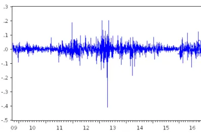
Fig. 5 – EUA Spot Price. Line & Symbol Eviews’ graph.
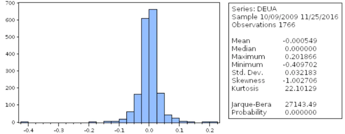
Furthermore, when considering the first difference of the logarithm (figure 6), it is even more clear the higher volatile period during the compliance brake. There are some other periods with high volatility, mainly during the first months, which might be related to the newly adjustments made by the regulators.
Table 2 in the appendix shows the plot of the 1st logarithm difference of the EUA prices. As common in other historical financial data, due the Kurtosis > 3 and Skewness 0, I reject the null hypothesis of the normality test for the dependent variable. In fact, this is a non-symmetric distribution, in the presence of a “leptokurtic” distribution or, in other words, fat tails, meaning it is more clustered around the mean.26 Moreover, the negative Skewness is emphasized on the left tail, i.e., the distribution is concentrated on the right side and the mode is greater than the arithmetic mean.
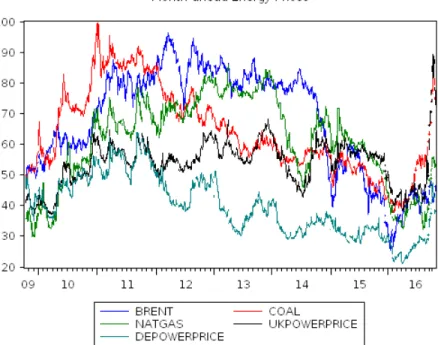
Regarding the energy based variables, figure 7 shows the distribution over time for the main variables under study. On the opposite of the EUA Spot price, the month-ahead prices for most of the energy independent variables show an upward trend during the 1st
compliance period and a downward trend during the 3rd phase. The significant drop in the ICE Brent Futures price, due to the 2014 oil crisis seems to drag other prices down, especially in the case of the natural gas due to the high correlation between both (table 3). In fact, it is expected due to the correlation between some regressors, e.g., Brent and Natural Gas is about 0.76 or, for the temperature indices correlation is about 0.61, some of the variables will not be statistical significant and need to be set apart of the final model.
Fig. 7 – Month-ahead energy prices.Line & Symbol Eviews’ graph.
Finally, table 4 in the appendix shows the descriptive statistics for each variable. While, for all the variables the normality null hypothesis is also rejected, which is in line with previous literature and it is rather common among economic data with bigger samples, the standard deviation is below 0.10 for all except for the temperature indices, which are not in the 1st logarithm difference. For the remaining results, I will consider 5% as my confidence interval.
These results are somehow surprising considering previous literature, which for example shows statistically significance levels for their weather. In my understanding, these means the simple dispersion of today’s observed temperatures against the mean temperature is not
a determinant factor of the EUA price. As adjustments were made in the core legislation of the EU ETS, it is fair to assume this effect was then corrected. Regardless further developments can be made to properly replicate the impact of such phenomenon.
In the next sections, I will start by analyzing the adjusted OLS regression for the whole period and then by splitting the sample and re-adjust the model, if necessary, for the remaining periods, in accordance with the methodology previously described.
9.1 OLS: whole sample 2009-2016
After dropping from eq. 1 the non-significant variables, the final OLS regression for the period under research is the following.
𝐷(𝑬𝑼𝑨) = 𝛼 + 𝛽𝐷(𝑩𝒓𝒆𝒏𝒕) + 𝛾𝐷(𝑪𝒐𝒂𝒍) + 𝜂𝐷(𝑷𝑷𝑫𝑬) + 𝜃𝐷(𝑷𝑷𝑼𝑲) + 𝜄𝐷(𝑪𝑫𝑺𝑫𝑬) + 𝜈𝐷(𝑺𝟔𝟎𝟎) + 𝜖 Equation 6 – OLS regression for the whole period.
The Baseload Power Price in Germany has a coefficient of 0.49, higher than all the remaining regressors, which emphasizes the EUA price dependence on the German market. There is also a negative correlation between the EUA price and the German Clean Dark Spread alongside with the CIF ARA Steam Coal price, which was also expected due to the simple logic that if the price of one of the raw materials associated with high emissions decreases, the EUA price increases in reaction to a cheaper access to it. Finally, the effects of institutional changes are still to be made, as it is not possible yet to analyze the impact on the EUA price within the whole period. For that, the next sections will provide a more concrete explanation.
9.2 OLS: second phase 2009 – 2013
For the 2nd phase of the EU ETS, the OLS regression shows an even lower R-squared value (0.08), meaning my regressors fail to properly explain the price movements between this period of the EUA price. Table 7 shows the OLS output generated by Eviews and, while it was fair to expect that more variables were statistically significant, the exact opposite happened. Only the German Baseload Power Price, the STOXX Europe 600 and the German Clean Dark Spread have a p-value lower than 2.5%.
The only apparent reason for these results is the downward trend observed from 2011 until the end of the 2nd phase. From 2011 until the end of the compliance period, the price dropped more than 38% and, if we consider the same metric just form May 2011 until November 2011, a 6-month period on which the price decreased almost 50%.
2009 until May 2011, the U.K. Clean Spark Spread is now statistically significant, while the macroeconomic proxy is not. The R-squared (table 8) increased to 0.14, which underlines the impact of the high percentage of free allocation during this period. Then, it is possible to assume that the EU as regulator had tremendous impact in the EUA price, which was highly expected considering it was still implementing and testing new safety measures to avoid price instability.
9.3 OLS: third phase 2013 – 2016
By avoiding the EU ETS highly unstable program during the 2nd phase, especially the downward trend mentioned before, I expect a more stable and self-explanatory model for the current stage. As so, table 8 in the appendix show the OLS regression outputs for the 3rd compliance period, from 2013 until the last observable date, 25th of November 2016.
Even considering the anomaly observed on May 2015, on which the EUA priced dropped to 0, the R-squared is slightly higher for the current compliance period (about 0.10). The ICE Brent Futures and CIF ARA Steam Coal are statistically significant once again, which is somehow surprising considering the oil crisis, which started in 2014.
volatility observed ended up to have a direct influence in the results. For future research on this topic, other proxies might be considered.
Even if the results are still underwhelming, the impact of the legislation amends on the EU ETS is still observable on the price volatility of the EUA secondary market, with a more stable upward pattern which was the main objective of regulators.
The next section concludes the OLS analysis by splitting the last compliance period per year, which will isolate external impacts previously highlighted.
9.4 OLS: third phase, year by year
plant, there is an evident incentive for producers to switch to a more cleaner energy source, resulting in the opposite coefficient shown in table 10.
To conclude the observations regarding 2013 OLS results, the more stable pattern of the EUA price, mainly due to the changes in the Cap size available, the incorporation of price constrain measures and the devolvement of auctions as the main tool obtain a permit allowed for other external variables to explain price movements better than before, underlining the widely expected importance of legislation on the EU ETS.
On the other hand, in 2014 the explanatory power of the OLS regression decreased to about 14%. While, the Natural Gas proxy variable was once again non-significant, the U.K. Baseload Power Price was also not significant due to its high p-value. For the first time in this research, both Clean Dark Spreads are significant within this period, emphasizing the importance of Steam Coal prices and the gross profit of power plants when accessing the settlement price of the EUA secondary market. It seems the driven power of such indices and variables is highly related with hedging purposes, as the largest emitters are necessary interested in securing their investment and profits. Finally, the beginning of the oil crisis has a direct impact on almost whole energy prices, especially on Natural Gas, which ultimately will influence the results, driving results to a lower level.
significant. The drop to zero in May 2015 is also non-relevant since, even if I exclude those two days, there is no increase in the explanatory power of the empirical model. The abnormal results are then purely related with changes in the external variables, since there were no legislative changes in the EU ETS and the pattern of the spot price seems stable enough to assume so.
Finally, for 2016 the results are astonishing high, with an R-squared of almost 45%. While the relative low number of observations (208) might indicate bias and higher results, there is no reason to think so as the time space used was close to the previous ones and if I extend the sample for 2-years period results remain high. Equation 12 shows the final OLS output with the substituted coefficients.
D(EUA) = 0.392186216059*D(BRENT) - 0.474599109907*D(COAL) + 0.834416065609*D(PPDE) +
0.206078281731*D(PPUK) - 0.0586547464128*D(CDSDE) + 0.0573712885302*D(SSUK)
Equation 7 – OLS estimation with substituted coefficients. Generated by Eviews.
and the reinforcement of price constrain measures on the EU ETS scope. Nevertheless, the remarkable high explanatory power of the model is beyond expected, especially considering the lower observed values for previous periods. While energy prices recover, I consider the more stable environment under the EU ETS to be also decisive, as non-institutional determinants gain more preponderance in explaining EUA price movements. 9.5 Robustness Tests
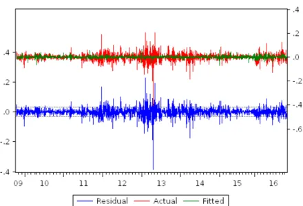
In accordance with section 7, to access the robustness and the viability of my model I will focus on testing the OLS residuals, generated for the whole period under study. Figure 8 below shows the OLS residuals plot generated with Eviews.
Fig. 8 – OLS residuals, actual and fitted.
Kurtosis > 3 and Skewness 0. As highlighted before, I expected this results due to the simple nature of the variables under study. For further research, the inclusion of dummy variables might help to correct for non-normality. Ultimately, a model which does not assumes normality could also be tested.
The Breusch-Godfrey Serial Correlation LM Test with 1 lag (table 15) shows that I do not reject the null hypothesis, p-value > 2.5%, meaning there is no serial correlation. This test allows to infer that, in principle, the coefficient estimates derived are not bias and the standard errors were appropriated generated. However, the inclusion of more than 1 lag violates the assumption that the variables are non-stochastic.
Figure 9 shows the test based on the recursive least squares residuals. While for most of the period, the confidence interval of the initial parameter covers the confidence interval for the remaining periods, it is possible to observe expected fluctuations around the compliance break due to the higher variance previously mentioned.
Fig. 9 – Recursive residuals tests generated by Eviews.
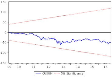
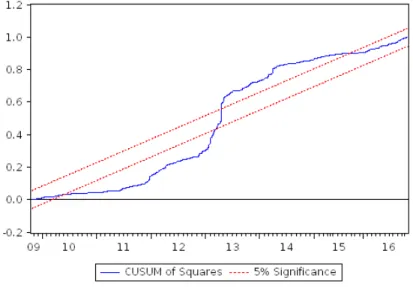
The CUSUM test (figure 10) makes a comparison between the cumulative sum of the standardized residual with 0. Since the parameters are constant, I cannot reject the null hypothesis, i.e., no break in the conditional mean.
However, it is important to notice that for almost the whole period values are negative.
To analyze the constant variance, I performed the CUSUM of Squares test (figure 11). The departures from the significance interval indicates a rejection of the null hypothesis, meaning that there might be a measurement error with the explanatory variables, i.e., they are non-stochastic and observations on independent variables are fixed in repeated samples.
Fig. 11 – CUSUM of Squares test, generated by Eviews.
The Ramsey RESET test (table 18) analyses the possibility of misspecification of functional form. Once again, due to the high p-value (about 0.34) I do not reject linearity.
10.
Conclusion
The results of this research show empirical evidence on the impact of several external variables on the EUA Spot Price. For the whole sample period, between 2009 and 2016, the price of the month-ahead Brent and Coal contracts, alongside with the Power Price practiced in Germany and in the U.K. are statistically significant, which is on line with previous literature. The economic growth proxy used, STOXX Europe 600 index is also significant, emphasizing the impact of the European economy on the EUA price and the Clean Dark Spread in Germany remains an important price drive factor during the whole period.
REFERENCES
McKibbin, Warwick J., et al. "Emissions trading, capital flows and the Kyoto Protocol." The Energy Journal (1999): 287-333.
Ellerman, A. Denny, and Barbara K. Buchner. "The European Union emissions trading scheme: origins, allocation, and early results." Review of environmental economics and policy 1.1 (2007): 66-87.
Schennach, Susanne M. "The economics of pollution permit banking in the context of Title IV of the 1990 Clean Air Act Amendments." Journal of Environmental Economics and Management 40.3 (2000): 189-210.
Convery, Frank J., and Luke Redmond. "Market and price developments in the European Union emissions trading scheme." Review of environmental economics and policy 1.1 (2007): 88-111.
Flachsland, Christian, Robert Marschinski, and Ottmar Edenhofer. "Global trading versus linking: Architectures for international emissions trading." Energy Policy 37.5 (2009): 1637-1647.
Böhringer, Christoph, Klaus Conrad, and Andreas Löschel. "Carbon taxes and joint implementation. an applied general equilibrium analysis for germany and india." Environmental and Resource Economics 24.1 (2003): 49-76.
Aatola, Piia, Markku Ollikainen, and Anne Toppinen. "Price determination in the EU ETS market: Theory and econometric analysis with market fundamentals." Energy Economics 36 (2013): 380-395.
Hintermann, Beat. "Allowance price drivers in the first phase of the EU ETS." Journal of Environmental Economics and Management 59.1 (2010): 43-56.
Keppler, Jan Horst, and Maria Mansanet-Bataller. "Causalities between CO 2, electricity, and other energy variables during phase I and phase II of the EU ETS." Energy Policy 38.7 (2010): 3329-3341.
Betz, Regina, and Misato Sato. "Emissions trading: lessons learnt from the 1st phase of the EU ETS and prospects for the 2nd phase." Climate Policy 6.4 (2006): 351-359.
Alberola, Emilie, Julien Chevallier, and Benoît Chèze. "Price drivers and structural breaks in European carbon prices 2005–
2007." Energy policy 36.2 (2008): 787-797.
Alberola, Emilie, and Julien Chevallier. "European carbon prices and banking restrictions: Evidence from Phase I (2005-2007)." The
Energy Journal (2009): 51-79.
Mansanet-Bataller, Maria, Angel Pardo, and Enric Valor. "CO₂ prices, energy and weather." The Energy Journal (2007): 73-92.
Christiansen, Atle C., et al. "Price determinants in the EU emissions trading scheme." Climate Policy 5.1 (2005): 15-30.
Alberola, Emilie, Julien Chevallier, and Benoît Chèze. "The EU emissions trading scheme: The effects of industrial production and CO2
emissions on carbon prices." Economie internationale 4 (2008): 93-125.
Declercq, Bruno, Erik Delarue, and William D’haeseleer. "Impact of the economic recession on the European power sector’s CO 2
emissions." Energy Policy 39.3 (2011): 1677-1686.
Kanen, Joost LM. “Carbon trading and pricing.”Environmental Finance Publications, 2006.
Hayes, Andrew F., and Li Cai. "Using heteroskedasticity-consistent standard error estimators in OLS regression: An introduction and
APPENDIX
Table 1 – Global Warming Potential Index. Source: Intergovernmental Panel on Climate Change.
GHG GLOBAL WARMING POTENTIAL
CARBON DIOXIDE 1
METHANE 25
NITROUS OXIDE 298
HYDROFLUROCARBONS 124 - 14,800 PERFLUORCARBONS 7390 - 12,200 SULFUR HEXAFLUORIDE 22,800 NITROGEN TRIFLUORIDE 17,200
Table 2 – Normality test of the 1st Logarithm difference of the EUA, generated with Eviews software.
Table 4 – Descriptive statistics, generated with Eviews.
Table 5 – OLS regression for the whole period and accounting with all dependent variables.
Table 7 – Adjusted OLS regression for the 2nd phase of the EU ETS.
Table 8 – Adjusted OLS regression from 2009 until May 2011.
Table 9 – Adjusted OLS regression for the third phase.
Table 11 – Adjusted OLS regression for the 2nd year of the 3rd phase.
Table 12 – Adjusted OLS regression for the 3rd phase, 2015.
Table 14 – Normality test of the OLS residuals.
Table 15 – Breusch-Godfrey Serial Correlation LM Test.
Table 17 – Heteroskedasticity Test: White test.