ScottKnott: A Package for Performing
the Scott-Knott Clustering Algorithm in R
E.G. JELIHOVSCHI1, J.C. FARIA2 and I.B. ALLAMAN3*
Received on January 18, 2013 / Accepted on February 18, 2014
ABSTRACT.Scott-Knott is an hierarchical clustering algorithm used in the application of ANOVA, when the researcher is comparing treatment means, with a very important characteristic: it does not present any overlapping in its grouping results. We wrote a code, in R, that performs this algorithm starting from
vectors, matrix, data.frame, aovoraov.listobjects. The results are presented with letters representing groups, as well as through graphics using different colors to differentiate distinct groups. This R package, namedScottKnottis the main topic of this article.
Keywords:Scott-Knott, multiple comparisons, R core team.
1 INTRODUCTION
Scott-Knott (SK) is a hierarchical clustering algorithm used as an exploratory data analysis tool. It was designed to help researchers working with an ANOVA experiment, wherein the compar-ison of treatment means is an important step in order, to find distinct homogeneous groups of those means whenever the situation leads to a significantF-test.
The multiple comparison procedures commonly used to solve this problem usually divide the set of treatment means into groups that are not completely distinct. Therefore, many treatments end up belonging to different groups simultaneously, this is called overlapping [6].
In fact, as the number of treatments increases, so do the number of overlappings making it dif-ficult for the experimental users to distinguish the real groups to which the treatments should belong. In this case, the division of treatments in completely distinct groups is the most impor-tant solution. Even though the goal of multiple comparison methods is an all-pair comparison, not a division of the treatment means into groups, biologists, plant breeders and many others expect those tests to make that divison in groups.
*Corresponding author: Ivan Bezerra Allaman
The possibility of using cluster analysis in place of multiple comparison procedures was sug-gested by [15] since the results of cluster type analysis, represent a type of solution for dividing treatments into distinct groups.
The SK algorithm is a hierarchical cluster analysis approach used to partition treatments into distinct groups. Many other hierarchical cluster analysis approaches have been proposed since Scott, A.J. and Knott, M. [18] published their results, such as, for example [13], [9], and [6]. However, the SK has been the most widely used approach due to its simple intuitive appeal, and also the good results it always provides [12, 4, 11, 14].
The SK procedure uses a clever algorithm of cluster analysis, where, starting from the whole group of observed mean effects, it divides, and keeps dividing the subgroups in such a way that the intersection of any of the two formed groups remains empty. In the words of A.J. Scott and M. Knott: “We study the consequences of using a well-known method of cluster analysis to partition the sample treatment means in a balanced design and show how a corresponding likelihood ratio test gives a method of judging the significance of the difference among groups obtained” [18]. Besides, simulation studies reveal that in comparison with the most used mul-tiple comparison procedures, the SK procedure has a very good performance [10, 5]. We also try to motivate the reader into the practice of the SK algorithm by bringing a real data example and compare the SK with other procedures, namely the clustering (hclust, packagestats) and Tukey test (packageagricolae).
The main objective of this paper is theScottKnottR package, which implements the SK proce-dure [18]. The package is available on the Comprehensive R Archive Network (CRAN) website and can be accessed at:http://CRAN.R-project.org/package=ScottKnott.
The R Package ScottKnottconsists of two methods,SKandSK.nest. TheSKmethod per-forms the algorithm on treatments of main factors whereasSK.nestdoes the same on nested designs of factorial, split-plot and split-split-plot experiments. They return objects of classes
SK, andSK.nestcontaining the groups of means plus other variables necessary forsummary
andplot. The generic functionssummaryandplotare used to obtain and print a summary and a plot.
Nowadays, the R environment for computational statistics has become the working language of computational statistics worldwide. Moreover, the huge processing power and memory space of modern computers has made it possible to write computer codes for almost every statistical methodology, indeed, this has eventually become, one of the main working tasks for statisticians and, as a result, statistical journals have been giving more space to the publication of software guides. Among them, the most important are the R packages.
2 REAL DATA STUDY
and 5 repetitions, that is, the yield of each treatment is measured 5 times. These data are available in theScottKnottpackage assorghum.
The objective of this study is to compare the 16 treatment means, as a first step of the whole analysis, and the question is: are there groups of treatments which could be considered homo-geneous? In other words, would it be possible to find groups for which the treatment means belonging to those groups that represent cultivars yielding the same weight of sorghum and the differences in the observed results being due to random variability?
We understand that this way of questioning is very important for the agricultural researcher and might be even more important than testing for the difference between treatment means for every pair of those means. There is a total of 120 of those pairs.
Even though this first study is just exploratory, it will give the researcher the insight he/she needs to continue the analysis.
This exploratory analysis was carried out using the SK algorithm, whose results were compared to two other methods.
> library(ScottKnott)
> data(sorghum)
> av <- aov(y ˜ r/bl + x,
+ data=sorghum$dfm)
> sk <- SK(av,
+ which=’x’,
+ sig.level=0.05)
> plot(sk,
+ title=NULL,
+ col=c(’black’,
+ ’gray’))
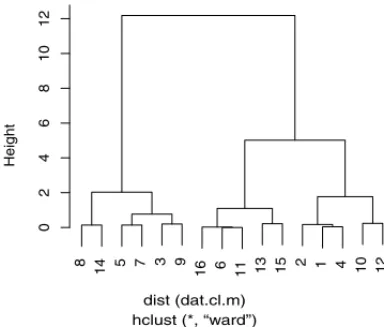
The first is the functionhclustfound in the packagestats, which performs hierarchical cluster analysis on a set of dissimilarities. The used agglomeration method was “ward”. We calculated the mean value of the 5 repetitions for each treatment and used it in thehclustfunction.
> dat.cl <- sorghum$dfm[order(sorghum$dfm$x), ][, 4]
> dim(dat.cl) <- c(5, 16)
> dimnames(dat.cl) <- list(paste(’r’,
+ 1:5,
+ sep=’’),
+ 1:16)
> dat.cl.m <- apply(dat.cl,
+ 2,
+ mean)
> cl <- hclust(dist(dat.cl.m),
+ ’ward’)
> plot(cl,
The second,was the Tukey’s HSD test which is a multiple comparison procedure that is also used by researchers to divide the treatment means into groups. We used the Rpackageagricolaeto build the graph.
> library(agricolae)
> tk <- HSD.test(av,
+ ’x’,
+ group=TRUE,
+ alpha=0.05)
> bar.group(tk$groups,
+ ylim=c(0, 12),
+ density=4,
+ border="black")
Figure 1 shows the result of the SK algorithm. It divided the means into two groups. The two main groups found using the functionhclust(Fig. 2) are not exactly the same as those found using the SK algorithm, but they are as similar as it was expected. The treatment means 14, 8, 5, 7, 9, 3 belong to the same group in both figures, and the treatments 1, 2, 4, which belong to the same group of the above treatments in Figure 1; in Figure 2, on the other hand, they belong to the second main group. Nevertheless, they are grouped together at the lowest level. Thehclustfunction cuts at the big gap between treatments 9 and 3 and the functionSKat the big gap between treatments 2 and 12.
Figure 3 shows the result using the Tukey’s HSD test. It finds 3 groups, marked by the letters a,bandc. Almost all of the treatments are classified to the 3 groups and this overlapping makes very difficult for the researcher to decide in which groups those means should be sorted.
What makes the SK algorithm more convenient in such cases is that, in addition to dividing the treatments in groups without overlapping, its result also uses a probabilistic approach aimed at finding the groups: the SK algorithm takes the maximum between group sum of squares, which is used in a likelihood ratio test with an asymptoticχ2distribution. This approach is very useful when the number of treatments is large.
It is also possible to change the value of the parametersig.levelof the SK function by getting different groupings, and the researcher can check what makes sense in practice.
3 COMPARATIVE PERFORMANCE OF SK METHOD
● ●
● ●
● ●
● ●
● ●
● ● ● ●
● ●
Groups
Means
3.6
5.9
8.2
10.6
12.9
14 8 5 7 9 3 1 4 2 12 10 16 6 11 13 15
Figure 1:Yield of sorghum using Skott-Knott algorithm,α=5%.
8
14 5 7 3 9 16 6 11 13 15 2 1 4 10 12
02468
1
0
1
2
Height
dist (dat.cl.m) hclust (*, “ward”)
Figure 2:Yield of sorghum using hclust, distance = euclidean and agglomeration method = ward.
14 8 5 7 9 3 1 4 2 12 10 16 11 6 13 15
02468
1
0
1
2
a ab
abc abc abc
abc
abc abc abc
abc abc
abc abc abc bc
c
Despite the fact that SK is a clustering procedure, we can use simulation results to compare its performance to Tukey test and others, as if it were a multiple comparison procedure.
Two of the most common measures to compare “Multiple Comparison Procedures” found in the literature are:
• The ratio between the number of type I errors (reaching the result thatµi =µj when truly
µi =µj) and the number of comparisons, is defined ascomparisonwise error rate.
• The ratio between the number of experiments with one or more type I errors and the total number of experiments is defined asexperimentwise error rate[7, 19].
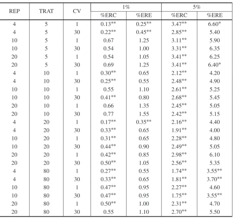
Two simulation studies conducted at the Federal University of Lavras, Brazil, used Monte Carlo methods to evaluate the performance of the SK method [3, 2]. One [10] showed that it possesses high power and an error rate that is almost always in accordance with the nominal levels using both comparisonwise and experimentwise error rates (Table 1). That is, the rates are not far from αvalue orsig.levelas defined in the last paragraph of section 4.1.
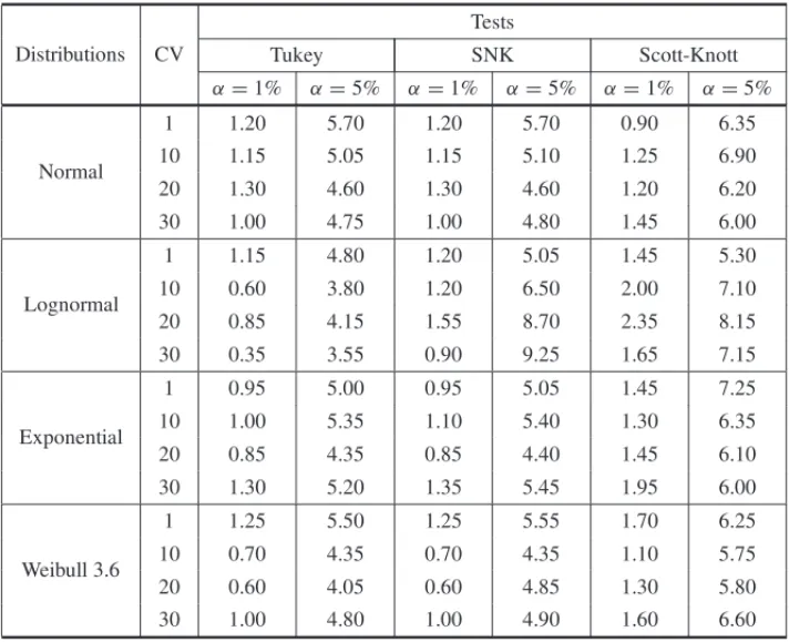
The other, [5] evaluated the power and the type I error rates of the SK, Tukey and SNK test, in a wide variety of experimental situations, in conditions of normality and non-normality error distribution (Table 2). They concluded that the SK is more powerful than the other two and is also robust against violations of normality assumptions. Both performed 2000 simulations for each experiment with 5, 10, 20 and 80 treatments with 4, 10 and 20 replicationsαvalue of 1% and 5% plus coefficients of variation of 1%, 10%, 20% and 30%.
4 METHOD
4.1 Methodology
Suppose we have a set of independent sample treatment means in the analysis of variance con-text, each treatment with the same number of replications, all normal variates, that is abalanced design. Furthermore, suppose that ANOVA leads to a significantF-testfor the difference among the treatment means. Moreover, by rejecting the homogeneity of the treatment means there is still the problem of finding out the number of homogeneous groups and which are the treatment means contained in each group.
It should be noted that we follow [6] in what we mean by homogeneity of treatments: “Once more it should be borne in mind that non rejection of equality is by no means equivalent to proving equality. We carefully defined homogeneity as non rejection of equality. Nor should it be inferred that treatments belonging to different “homogeneous groups” are (significantly) different; treatments belonging to the same group, however, are not.” The SK procedure is a hierarchical clustering algorithm that attempts to find out those groups without overlapping.
Table 1: Error rates by comparisons (ERC) and experiment (ERE), for the Scott-Knott test, de-pending on the number of repetitions (REP), number of treatments (TRAT), coefficient of variation (CV) and nominal levels of significance atα=1% andα=5%.
REP TRAT CV 1% 5%
%ERC %ERE %ERC %ERE
4 5 1 0.13∗∗ 0.25∗∗ 3.47∗∗ 6.60∗ 4 5 30 0.22∗∗ 0.45∗∗ 2.85∗∗ 5.40
10 5 1 0.67 1.25 3.11∗∗ 5.90
10 5 30 0.54 1.00 3.31∗∗ 6.35
20 5 1 0.54 1.05 3.41∗∗ 6.25
20 5 30 0.69 1.25 3.41∗∗ 6.40∗
4 10 1 0.30∗∗ 0.65 2.12∗∗ 4.20
4 10 30 0.25∗∗ 0.55 2.48∗∗ 4.90
10 10 1 0.55 1.10 2.61∗∗ 5.25
10 10 30 0.41∗∗ 0.80 2.68∗∗ 5.45
20 10 1 0.66 1.35 2.45∗∗ 5.05
20 10 30 0.77 1.55 2.42∗∗ 5.15
4 20 1 0.17∗∗ 0.35∗∗ 2.16∗∗ 4.40
4 20 30 0.33∗∗ 0.65 1.91∗∗ 4.00
10 20 1 0.31∗∗ 0.65 2.28∗∗ 4.80
10 20 30 0.44∗∗ 0.90 2.49∗∗ 5.05
20 20 1 0.42∗∗ 0.85 2.98∗∗ 6.10
20 20 30 0.50∗∗ 1.05 2.56∗∗ 5.35
4 80 1 0.27∗∗ 0.55 1.74∗∗ 3.55∗∗ 4 80 30 0.33∗∗ 0.65 1.81∗∗ 3.70∗∗
10 80 1 0.47∗∗ 0.95 2.27∗∗ 4.60
10 80 30 0.47∗∗ 0.95 1.75∗∗ 3.55∗∗
20 80 1 0.50∗∗ 1.00 2.31∗∗ 4.70
20 80 30 0.55 1.10 2.70∗∗ 5.50
Source: Adapted of [10].∗Exceeded the upper limit of the confidence interval accurate, with 99% confidence to
nominal levels of significance of 1% (1.727044) and 5% (6.391386).∗∗Exceeded the upper limit of the confidence interval accurate, with 99% confidence to nominal levels of significance of 1% (0,518787) and 5% (3,828164).
homogeneous belonging to just one group. To do so, it should divide the 2k−1−1 possible partitions of thekmeans in two nonempty groups, but it is enough to look at thek−1 partitions formed by ordering the treatment means and divide them between two successive ones [18]. Let T1 andT2 be the totals of two of those groups withk1 andk2 treatments in each one, so that
k1+k2=k, that is:
T1=
k1
i=1
y(i) T2=
k1+k2
i=k1+1
y(i)
Table 2:Type I error rates by experiment (%), to the Tukey, SNK and Scott Knott tests, for different CV and distributions, considering the number of treatments (p) equal to 10 and 20 replications for nominal levels of significance 1% to 5%.
Distributions CV
Tests
Tukey SNK Scott-Knott α=1% α=5% α=1% α=5% α=1% α=5%
Normal
1 1.20 5.70 1.20 5.70 0.90 6.35 10 1.15 5.05 1.15 5.10 1.25 6.90 20 1.30 4.60 1.30 4.60 1.20 6.20 30 1.00 4.75 1.00 4.80 1.45 6.00
Lognormal
1 1.15 4.80 1.20 5.05 1.45 5.30 10 0.60 3.80 1.20 6.50 2.00 7.10 20 0.85 4.15 1.55 8.70 2.35 8.15 30 0.35 3.55 0.90 9.25 1.65 7.15
Exponential
1 0.95 5.00 0.95 5.05 1.45 7.25 10 1.00 5.35 1.10 5.40 1.30 6.35 20 0.85 4.35 0.85 4.40 1.45 6.10 30 1.30 5.20 1.35 5.45 1.95 6.00
Weibull 3.6
1 1.25 5.50 1.25 5.55 1.70 6.25 10 0.70 4.35 0.70 4.35 1.10 5.75 20 0.60 4.05 0.60 4.85 1.30 5.80 30 1.00 4.80 1.00 4.90 1.60 6.60
Source: [5].
Also, letBbe the between groups sum of squares. That is:
B = T
2 1
k1
+T
2 2
k2
−(T1+T2)
2
k1+k2
LetBobe the maximum value, taken over thek−1 partitions of thektreatments into two groups, of the between groups sum of squares B. After finding out those groups, we use the likelihood ratio test for the null hypothesis of equality of all means against the alternative that they belong to the two groups found above. If we reject this hypothesis then the two groups are kept, other-wise the group ofktreatment means is considered homogeneous. We then repeat this procedure for each group separatly and stop until all of the formed groups become homogeneous.
The statistics used for the likelihood ratio test is:
λ= π
2(π −2)×
Bo
σ2
o
Lets2 = M S Er be the unbiased estimator of σr2,υ be degrees of freedom associated with that estimator, then
σo2=
k
i=1(y(i)−y)2+υs2
k+υ
λis asymptotically aχ2distributed random variable withυo= πk−2degrees of freedom. There-fore we can use that to set the cutoff point for a givenαvalue each time we perform the test.
We can think the p-value of likelihood ratio test as a distance to be measured between the two selected groups and the type I error (αvalue) chosen to be the cut off. If the p-value is smaller thanα, the groups are too far away from each other and should be separated (they are heteroge-neous), otherwise, they become just one group (homogeneous).
“Choosing an appropriate value forα is difficult. Ifα is too small, the splitting process will terminate too soon, on the other hand, ifα is too large, the process will go too far and split homogeneous sets of means” [18].
As we start dividing the first groups into other smaller groups, we repeat the same algorithm for each group. We keep doing that until every formed group is either homogeneous or just contains one observed mean.
It is important to emphasize the fact that the above definedαvalue is not the nominal error rate of the type I error of the algorithm as a whole. If we set theαvalue as 5% then every test the SK procedure performs to divide (or not) a sub-group has a type I error rate of 5%. Nevertheless, we cannot say that the former type I error rate is 5%. Thisαvalue is the parameter calledsig.level in the SK function.
4.2 ScottKnott package
The ScottKnottpackage was written in R language [17]. The results are objects of the class
list,SKandSK.nest, which are used as an input to the generic functionssummaryand
plot. It performs the clustering algorithm on three designs and three experiments. Once again, it must be emphasized again that the two functions SK and SK.nest only work on bal-anced designs. The designs are: Completely Randomized Design (CRD), Randomized Complete Block Design (RCBD) and Latin Squares Design (LSD). The experiments are: Factorial Experi-ment (FE), Split-Plot ExperiExperi-ment (SPE) and Split-Split-Plot ExperiExperi-ment (SSPE).
The ScottKnott package has two main functions:SK andSK.nest. The SK functionis used for clustering the treatment means of a main factor. TheSK.nestfunction, in turn, is used for clustering treatment means relative to interactions among factors, that is whenever the treatment means belong to a factor nested in others. For example, the treatment means of factor A, for level 1 of factor B, and level 1 of factor C. As shown above, theSK.nest function
supports no more than two nestings.
The main algorithm is theMaxValuefunction which builds groups of means according to the method of SK. It is basically an algorithm for a pre-order path in a binary decision tree. Every node of this tree, represents a different group of means and, when the algorithm reaches this node it takes the decision to either split the group in two, or to form a group of means. At the end all the leaves of the tree are the groups of homogeneous means.
TheSKandSK.nestfunctions are methods for objects of classvector,matrix or data. framejoined as default, whereasaovandaovlistare methods for single experiments.
The main parameters used by those methods are:
• x: A design matrix,data.frameor anaovobject.
• y: A vector of response variable. It is only necessary to inform this parameter ifx repre-sents the design matrix.
• which: The name of the factor to be used in the clustering. The name must be inside quoting marks.
• model: Ifxis adata.frameobject, the model to be used in the aov must be specified.
• error: The error to be considered. Only used in cases ofsplit-plotorsplit-split-plot exper-iments.
• sig.level: Level of Significance,αvalue, used in theSKandSK.nestalgorithms to create the groups of means. The default value is 0.05.
• f l1: A vector of length 1 providing the level of the first factor in the tested nesting order.
• f l2: A vector of length 1 providing the level of the second factor in the tested nesting order.
• id.trim: The number of characters to trim the label of the factor levels.
• . . . : Further arguments (required by generic).
4.2.1 Split-Split-Plot Experiment (SSPE)
We show an example on how to use theScottKnottpackage. An object ofaovlistclass will be used in the SK.nest function.
SSPE is the objet containing the data set for a Split-Split-Plot Experiment (SSPE). It is a simu-lated data aimed at modelling a SSPE with 3 plots, each one split 3 times, each split, split again 5 times and 4 repetitions per split-split.
It can be called using the command below:
> data(SSPE)
> nav <- with(SSPE,
+ aov(y ˜ blk + P*SP*SSP + Error(blk/P/SP),
SSPfactor is nested inSPfactor, which is nested inPfactor. The value 1 of the parameter f l1 and 1 of parameter f l2mean that the first level of factorsPandSP, respectively, are chosen. The comparison is made only among levels (treatments) of factorSSPbelonging to that par-ticular combination of levels of factorPand factorSP. Look at the aov(model) andSK.nest
(which) functions for the order at which the factors appear.
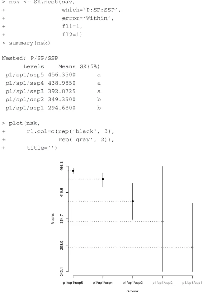
> nsk <- SK.nest(nav,
+ which=’P:SP:SSP’,
+ error=’Within’,
+ fl1=1,
+ fl2=1)
> summary(nsk)
Nested: P/SP/SSP
Levels Means SK(5%)
p1/sp1/ssp5 456.3500 a
p1/sp1/ssp4 438.9850 a
p1/sp1/ssp3 392.0725 a
p1/sp1/ssp2 349.3500 b
p1/sp1/ssp1 294.6800 b
> plot(nsk,
+ rl.col=c(rep(’black’, 3),
+ rep(’gray’, 2)),
+ title=’’)
●
●
●
●
●
Groups
Means
243.1
298.9
354.7
410.5
466.3
p1/sp1/ssp5 p1/sp1/ssp4 p1/sp1/ssp3 p1/sp1/ssp2 p1/sp1/ssp1
Figure 4:Split-Split-Plot Experiment (SSPE). Nested analysis (ssp/sp=1/p=1),α=5%.
5 THE PACKAGE USAGE
The best measurement of how much the ScottKnott package is used around the world is to count the number of times it has been downloaded since it became available at the CRAN (The Com-prehensive R Archive Network). Unfortunately, only one (http://cran-logs.rstudio. com), out of 88 mirrors, has control of downloads. Therefore, the numbers shown below are very underestimated. Two other factors contribute with that underestimation: the download control effected by that mirror began on October 1, 2012 and the ScottKnott package has been avail-able since January 2009, and second, this mirror is not Brazilian, whereas Brazilian statisticians are those who mostly use the ScottKnott method. In any case, a little information is better than none at all.
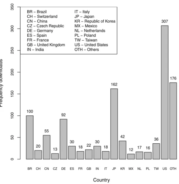
Figure 5 lists the countries that have downloaded the ScottKnott package between periods from October 1, 2012 to August 30, 2013. The country with the highest number of downloads is the United States. The “other” category comprises 55 countries with the number of downloads below 10.
BR CH CN CZ DE ES FR GB IN IT JP KR MX NL PL TW US OTH
Country Frequency do wnloads 0 50 100 150 200 250 300 350
BR − Brazil CH − Switzerland CN − China CZ − Czech Republic DE − Germany ES − Spain FR − France GB − United Kingdom IN − India
IT − Italy JP − Japan KR − Republic of Korea MX − Mexico NL − Netherlands PL − Poland TW − Taiwan US − United States OTH − Others
100 20 55 13 92 30 18 22 30 18 162 42
12 17 16 36
307
176
Figure 5: Number of downloads of the ScottKnott package by countries between October 1, 2012 and August 30, 2013.
Date (Year−Month)
Frequency do
wnloads
2012−10 2012−11 2012−12 2013−01 2013−02 2013−03 2013−04 2013−05 2013−06 2013−07 2013−08
0
50
100
150
200
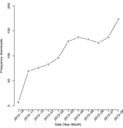
Figure 6:Number of downloads of the ScottKnott package between October 1, 2012 and August 30, 2013.
6 CONCLUSION
The Scott and Knott (SK) algorithm is a very useful methodology in the practice of statistical analysis of experiments involving of analysis of variance. It has been widely used by researchers who wish to compare the group means of treatments, since it divides groups without any over-lapping, a feature that makes the algorithm very useful. The R package ScottKnott provides an easy-to-use framework for performing the SK algorithm. In comparison with other software or Rpackages, this one is unique unto itself, since it allows for easily interpreting of graphics results, what greatly facilitates the interpretation of analyses. As explained in the article, it also makes possible various designs and experiments.
ScottKnot is still undergoing active development. Planned extensions include extension of the method to factorial up to fifth order, methods using poisson distribution, dendrogram graphic option with p-values obtained for each group, and an alternative method of the Scott-Knott test proposed by [1].
gr´aficos usando cores diferentes para diferenciar os grupos distintos. Este pacote do R, nomeadoScottKnott´e o principal tema deste artigo.
Palavras-chave:Scott-Knott, comparac¸˜oes m´ultiplas, R core team.
REFERENCES
[1] L.L. Bhering, C.D. Cruz, E.S. De Vasconcelos, A. Ferreira & M.F.R. De Resende Jr. Alternative methodology for Scott-Knott test.Crop Breeding and Applied Biotechnology,8(2008), 9–16. [2] C.S. Bernhardson. Type I error rates when multiple comparison procedure follow a significant F
test of ANOVA.Biometrics,31(1) (1975), 337–340.
[3] T.J. Boardman & D.R. Moffit. Graphical Monte Carlo Type I error rates for multiple comparison procedures.Biometrics,27(3) (1971), 738–744.
[4] S. Bony, N. Pichon, C. Ravel, A. Durix, F. Balfourier & J.J. Guillaumin. The Relationship between Mycotoxin Synthesis and Isolate Morphology in Fungal Endophytes of Lolium perenne.New Phytol-ogist,152(1) (2001), 125–137.
[5] L.C. Borges & D.F. Ferreira. Power and type I errors rate of Scott-Knott, Tukey and Newman-Keuls tests under normal and no-normal distributions of the residues.Revista de Matem´atica e Estat´ıstica, 21(1) (2003), 67–83.
[6] T. Calinski & L.C.A Corsten. Clustering Means in ANOVA by Simultaneous Testing.Biometrics, 41(1) (1985), 39–48.
[7] S.G. Carmer & M.R. Swanson. Detection of differences between means: a Monte Carlo study of five pairwise multiple comparison procedures.Agronomy Journal,63(6) (1971), 940–945.
[8] S.G. Carmer & M.R. Swanson. An evaluation of ten pairwise multiple comparison procedures by Monte Carlo methods.Journal American Statistical Association,68(1973), 66–74.
[9] D.R. Cox & E. Spjotvoll. On partitioning means into groups.Scandinavian Journal of Statistics, 9(1982), 147–152.
[10] E.C. Da Silva, D.F. Ferreira & E. Bearzoti. Evaluation of power and type I error rates of Scott-Knott’s test by the method of Monte Carlo.Ciˆencias Agrot´ecnicas.,23(1999), 687–696.
[11] A.B. Dilson, S.D. David, J. Kazimierz & W.K. William. Half-sib progeny evaluation and selection of potatoes resistant to the US8 genotype of Phytophthora infestans from crosses between resistant and susceptible parents.Euphytica,125(2002), 129–138.
[12] C.E. Gates & J.D. Bilbro. Illustration of a Cluster Analysis Method for Mean Separation.Agron J, 70(1978), 462–465.
[13] I.T. Jollife. Cluster analysis as multiple comparison method.Applied Statistics. RP Gupta (ed): 159– 168, North Holland, (1975).
[14] S. Jyotsna, L.W. Zettler, J.W. van Sambeek, Ellersieck & C.J. Starbuck. Symbiotic Seed Germination and Mycorrhizae of Federally Threatened Platanthera Praeclara(Orchidaceae).American Midland Naturalist,149S(1) (2003), 104–120.
[16] M.A.P. Ramalho, D.F. Ferreira & A.C. Oliveira.Experimentac¸˜ao em Gen´etica e Melhoramento de Plantas. Editora UFLA, Lavras, (2000).
[17] R Development Core Team.R: A Language and Environment for Statistical Computing.R Foundation for Statistical Computing, Vienna, Austria, 2010. ISBN 3-900051-07-0.
[18] A.J. Scott & M. Knott. A cluster analysis method for grouping means in the analysis of variance. Biometrics,30(1974), 507–512.