On Convergence and Solvability of an Elliptic Equation
by Finite Difference Method
A.J.A. RAMOS
Received on September 1, 2016 / Accepted on December 9, 2016
ABSTRACT.In this article we deal with questions of convergence, existence and uniqueness of the numer-ical solutions for a discretized elliptic problem by using finite difference method. In order to show existence and uniqueness of numerical solutions we will use a suitable variational setup (at discrete level) to guarantee the existence of a numerical solution by means of a finite difference method.
Keywords:elliptic equation, finite difference, solvability of numerical solutions.
1 INTRODUCTION
It is well known that the general model
−u+q(x)u = f(x) in ,
u = 0 on ∂, (1.1)
whereq, f ∈ C()has been vastly studied in the last years. See, for example, [1, 2, 3, 4] and the references therein.
Here,⊂RN, N ≥1 is a bounded smooth domain and f :→ Ris a given function has
relevant physical motivation as, for instance, stationary solutions of heat and wave equations, population models and geometric models and so on. Besides of this we have several nonlocal models like
−M(B(u))u+q(x)u = f(x) in ,
u = 0 on ∂, (1.2)
whereMis a given function andBis an integral operator, is also of paramount importance in the modeling of several phenomena. In a forthcoming paper we will attack this last problem.
Let us recall some known results on existence and uniqueness of solutions to the problem (1.1). This is important for aims that we have in mind.
The problem (1.1) is so-called the homogeneous Dirichlet problem. Generally speaking, the Dirichlet problem consists in coupling a differential equation with a boundary condition that specifies the values of the unknown function on the boundary of; one says that the Dirichlet condition is homogeneous if the unknown is required to be zero on∂.
Let us takeq ∈L∞()and f ∈L2(). It is well know that a weak solution of problem(1.1)is a functionu ∈H01()such that
∇u· ∇vd x+
q(x)uvd x=
f(x)vd x, ∀v∈H01(). (1.3)
As consequence of this variational formulation, we define the functionalJ :H01()→Rgiven
by
J(u):= 1
2
|∇u|2d x+1
2
q(x)|u|2d x−
f(x)vd x. (1.4)
This functional is often called the energy functional associated to problem(1.1)in its importance relies from applications, where J is likely to represent an energy of some sort. Moreover, it is well known that the functionalJis differentiable onH01()and its derivative is given by
J′(u)v =
∇u· ∇vd x+
q(x)uvd x (1.5)
−
f(x)vd x, ∀v∈H01().
Therefore, comparing(1.3)and(1.5), one sees that the functionsuis a weak solution of problem
(1.1)if and only ifu is a critical point of the functional J. Furthermore it is shown thatJ is continuous, coercive and strictly convex which ensures the existence of global minimum point and consequently existence and uniqueness of solution to the problem (1.1).
1.1 Numerical setting and statement of the results
In this work, we are concerned with a discrete version of the problem (1.1) at numerical setting of the finite differences. Here, we take⊂R2.
More precisely, we consider the following numerical scheme:
Ldui,j = fi,j, 0≤i ≤N, 0≤ j≤ M, ind,
ui,0=u0,j = 0, 0≤i ≤ N+1, 0≤ j≤ M+1,
(1.6)
where we are assuming that
Ldui,j := −dui,j +qi,jui,j, (1.7)
where
dui,j :=
ui+1,j−2ui,j +ui−1,j
x2 +
ui,j+1−2ui,j +ui,j−1
The numerical operator (1.8) is the finite difference operator centered for the 2ndorder derivative, known as five points formula. Here, the discrete solutionsui,j andvi,j are approximations to
u(xi,yj)andv(xi,yj)at the mesh points(xi,yj), respectively.
Moreover,qi,j ∈l∞(d)and fi,j ∈l02(d). The spacel02(d)is defined as
l02(d)=
ui,j :d →R;
N
i=0
M
j=0
|ui,j|2
1/2
<∞
, (1.9)
satisfyingui,0 =u0,j =0, for all 0≤i ≤ N +1 and 0 ≤ j ≤ M+1. This discrete space is
equipped with the inner product and the norm given, respectively, by
ui,j, vi,j
l2(
d)
= xy
M
j=0
N
i=0
ui,jvi,j, (1.10)
|ui,j|l2(
d) = ui,j,ui,j
1/2
l2(
d)
. (1.11)
Moreover, we defined other inner product as
∇ui,j,∇vi,j
= xy
N
i=0
M
j=0
∇xui,j · ∇xvi,j (1.12)
+ xy
N
i=0
M
j=0
∇yui,j · ∇yvi,j,
and norm as
||∇ui,j|| =
∇ui,j,∇ui,j
1/2
. (1.13)
In (1.12), we have used the numerical operators given by
∇xui,j :=
ui+1,j −ui,j
x , ∇yui,j :=
ui,j+1−ui,j y .
Moreover, the spacel0∞(d)is defined as being the discrete space of the real bounded sequences
l∞0 (d)=
ui,j :d →R; sup
0≤i,j≤N,M
|ui,j|<∞
, (1.14)
obeyingui,0=u0,j =0, for all 0≤i ≤ N+1, 0≤ j ≤ M+1. This space is equipped with
the norm
||ui,j||∞= sup 0≤i,j≤N,M
The discrete domain d is given by a discretization of the rectangle [0,L1] × [0,L2]. We consider a discretization of the intervals[0,L1]and[0,L2]given by
0 = x0<x1< . . . <xi =ix < . . . <xN <xN+1=L1, 0 = y0<y1< . . . <yj = jy< . . . <yM <yM+1=L2,
wherex=L1/(N+1),y=L2/(M+1)andN,M ∈N. Hence,
d= N,M
i,j=0
(xi,xi+1)×(yj,yj+1) and lim
x,y→0d =(0,L1)×(0,L2).
The main results of this paper are as follows:
Theorem 1.1.Let=(0,L1)×(0,L1)and u∈C4()be a classical solution of the Dirichlet
problem
−u+q(x)u = f(x), in ,
u = 0, on ∂, (1.16)
whered ⊂is a discrete domain and ui,j a corresponding solution of the discretized problem
Ldui,j = fi,j, 0≤i≤ N,0≤ j ≤M, ind,
ui,0 =u0,j = 0, 0≤i≤ N+1, 0≤ j ≤M+1.
(1.17)
Then, there exists a positive constant C independent of u satisfying the following estimate:
||u(xi,yj)−ui,j||∞≤C||D4u||L∞()(x2+y2). (1.18)
Theorem 1.2. Letd ⊂ [0,L1] × [0,L2]be a discrete domain. Assuming qi,j ∈l∞(d)and
fi,j ∈l02(d), then there exists only one solution of the discrete problem (1.17).
We highlight some observations on numerical convergence. When we deal with parabolic prob-lems like
uni,+j1−uni,−j1 2t −
uni+1,j−2uin,j +uni−1,j
x2 −
uni,j+1−2uin,j +uni,j−1
y2 = fi,j, (1.19)
the convergence analysis is performed through the condition CFL (Courant-Friedrichs-Lewy), where the numerical stability is verified accordingly a Von Neumann condition (see [5]). It is clear that, in the elliptic case, we are not able to use the same arguments. Because of this, we use certain tools typical of elliptic equations, likeDiscrete Maximum Principle(see Section 10.3 of Thomas [6]) in order to guarantee the a priori estimate and, consequently, to reach in the numerical convergence of the Poisson problem
−ui+1,j −2ui,j +ui−1,j
x2 −
ui,j+1−2ui,j+ui,j−1
Still concerning with the Poisson problem, the proof of the existence and uniqueness of the discrete solution, given in [7, 6, 8], consists in showing that the matrix
A=
⎛ ⎜ ⎜ ⎜ ⎜ ⎜ ⎜ ⎜ ⎜ ⎜ ⎜ ⎜ ⎝
B − 1
y2I
− 1
y2I B − 1
y2I
− 1
y2I . .. . ..
. .. . .. − 1
y2I
− 1
y2I B − 1
y2I
− 1
y2I B ⎞ ⎟ ⎟ ⎟ ⎟ ⎟ ⎟ ⎟ ⎟ ⎟ ⎟ ⎟ ⎠
(M−1)×(M−1)
associated to the numerical problem, whereI is the(N −1)×(N−1)identity matrix andB uma matriz tridiagonal(N−1)×(N−1), is a positive definite symmetric matrix and in order to obtain invertibility we should have.
Here we use a technique which is not usual in this kind of problem. Indeed, following ideas similar to those used in continuous case, we consider a variational approach at discrete setting. In this way we consider an discrete functional in such a way their critical points are weak solutions of our problem.
Our approach is this work is twofold. Firstly, we focus on the existence of an priori estimate in order to guarantee the convergence of the numerical solution. Secondly, we build a discrete func-tional in order to prove the existence and uniqueness of solution for the discrete problem (1.6).
1.2 Outline of the paper
The plan of this paper is as follows: in Section 2 we establish the convergence of numerical solutions. In particular, we proved a discrete version to the Maximum Principle. In Section 3 we treated a variational formulation in numerical setting and in Section 4 we prove our main results. Finally, in Section 5, we proved with numerical experiments some of these results.
2 CONVERGENCE OF THE DISCRETE SOLUTION
In this section, we prove aDiscrete Maximum Principleplaying an important role in the proof of the a priori estimate for solutions of the problem (1.6). Moreover, we prove a result on estimative a priori of the discrete solution of our problem.
Theorem 2.1 (Discrete Maximum Principle).Let
Ldui,j := −dui,j +qi,jui,j ≤(≥)0, in d. (2.1)
Proof. To proof our assertive, we consider that the maximum ofui,j is not attained in∂d.
First we note thatLdui,j ≤0 is equivalent with
1
x2 + 1
y2 + qi,j
2
ui,j ≤
1
2x2(ui+1,j +ui−1,j) (2.2)
+ 1
2y2(ui,j+1+ui,j−1)
for all 0≤i ≤N, 0≤ j≤ M.
Suppose thatui,j is the local maximum. Then, for all indicesi = 0,N+1, j =0,M+1 we
have
ui,j ≥ui+1,j, ui,j ≥ui−1,j, ui,j ≥ui,j+1 and ui,j ≥ui,j−1.
Taking into account these inequalities, we can rewritten (2.2) as
1
x2 + 1
y2 + qi,j
2
ui,j ≤
1 2
1
x2ui+1,j+ 1
x2ui,j + 2
y2ui,j
≤
1
x2 + 1
y2
ui,j,
from where we have, sinceqi,j ≥0 for all 0≤i ≤N, 0≤ j≤ M,
1
x2 + 1
y2
ui,j ≤
1 2
1
x2ui+1,j+ 1
x2ui,j + 2
y2ui,j
≤
1
x2 + 1
y2
ui,j,
and then
1
x2ui,j = 1 2
1
x2ui+1,j + 1
x2ui,j
,
and, consequently,
ui+1,j =ui,j, ∀i =0,N+1, j =0,M+1.
Reasoning in the same way, we get
ui,j =ui+1,j =ui−1,j =ui,j+1 =ui,j−1, ∀i=0,N+1, j =0,M+1. (2.3)
This shows thatui,j is a constant function which obviously is a contradiction and therefore the
maximum is attained on the boundary. The proof of the minimum principle is performed in the
same way.
Now, without loss of generality, we considerL1= L2 =1 and we will work in the unit square
=(0,1)×(0,1). We will use the discrete sup norm for functions defined in the discretized domaind, that is,
||ui,j||∞=max
i,j∈N
At first we obtain a priori estimate, which may be seen as a discrete regularity result, for solutions of a homogeneous discrete Dirichlet problem.
Theorem 2.2 (A Priori Estimate).Let ui,j be a solution of discrete system (1.6). Then, we have
||ui,j||∞≤ ||Ldui,j||∞, ∀i,j, (2.5)
whereLdui,j = −dui,j +qi,jui,j and 0≤qi,j ∈l∞(d).
Proof. Let us consider the discrete functionwi,j defined as
wi,j :=
1 4
xi−
1 2
2
+
yj −
1 2
2
≥0, ∀i,j, (2.6)
with||qi,j||∞<||wi,j||−∞1.For this function we statement that
−1≤Ldwi,j ≤ −1+||qi,j||∞
8 , ∀i,j. (2.7)
Indeed, we have
Ldwi,j = −1
4
(xi+1−12)2+(yj −12)2−2(xi−12)2−2(yj−12)2 x2
− 1
4
(xi−1−12)2+(yj−12)2 x2
− 1
4
(xi−12)2+(yj+1−12)2−2(xi −12)2−2(yj−12)2 x2
− 1
4
(xi−12)2+(yj−1−12)2
x2
+ qi,j
4 xi− 1 2
2
+ yj −
1 2
2
.
Ldwi,j = −
1 4
(xi+1−12)2−2(xi−12)2+(xi−1−12)2
x2
+ 1
4
(yj+1−12)2−2(yj −12)2+(yj−1−12)2
y2
+ qi,j
4 xi− 1 2
2
+ yj −
1 2
2
Ldwi,j = −1
4
(xi+x−12)2−2(xi−12)2+(xi−x−12)2 x2
− 1
4
(yj +y−12)2−2(yj−12)2+(yj−y−12)2 y2
+ qi,j
4 xi− 1 2
2
+ yj −
1 2
2
Consequently, we obtain
−1≤Ldwi,j = −1+qi,j
4 xi− 1 2
2
+ yj −
1 2
2
≤ −1+||qi,j||∞
4
max 0≤xi≤1
xi −
1 2
2
+ max
0≤yj≤1
yj−
1 2
2
= −1+||qi,j||∞
8 .
Now, let us assume that||qi,j||∞=7<||wi,j||−∞1, from where we obtain
−1≤Ldwi,j ≤ −1
8,
and then we can define
Ldwi,j = −ξi,j ∈I, ξi,j ≥0,
for 0 ≤i ≤ N+1, 0≤ j ≤ M+1 andI =−1,−1/8. Moreover, we define the discrete functional
g±i,j :l02(d)×l02(d) → R
(ui,j, wi,j) → gi±,j =ui,j ±8||Ldui,j||∞wi,j.
to obtain
Ldg−
i,j = Ld(ui,j −8||Ldui,j||∞wi,j)=Ldui,j −8||Ldui,j||∞Ldwi,j = Ldui,j +8ξi,j||Ldui,j||∞≥0,
form where by using the Maximum Principle that the functiongi−,j attains its minimum value at the boundary. In view of this we get
ui,j ≥gi−,j ≥ −8||Ldui,j||∞max
∂d
wi,j,
and from definition ofwi,j em(2.6)we obtain max
∂d
wi,j =
1
8 and then
ui,j ≥ −||Ldui,j||∞, 1≤i ≤ N, 1≤ j ≤M. (2.8)
In the same way, it follows that the functiongi+,j attains its maximum at the boundary, that is,
ui,j ≤ ||Ldui,j||∞, 1≤i≤ N, 1≤ j ≤ M. (2.9)
Combining the inequalities(2.8)and(2.9)it follows that
|ui,j| ≤ ||Ldui,j||∞, ∀1≤i ≤ N, ∀1≤ j ≤ M, (2.10)
3 VARIATIONAL FORMULATION AND THE SPECTRUM AT DISCRETE SETTING
In this section, we are concerned with discrete solutions of the discrete problem (1.6) satisfying a summable identity. In this way we have the following result:
Theorem 3.1. Let us consider qi,j ∈ l∞(d)and fi,j ∈ l2(d). The discrete solution of the
problem (1.6) obeys the following identity:
xy
N
i=0
M
j=0
∇xui,j · ∇xvi,j
+xy
N
i=0
M
j=0
∇yui,j · ∇yvi,j
+xy
N
i=0
M
j=0
qi,jui,jvi,j =xy N
i=0
M
j=0
fi,jvi,j, ∀vi,j ∈l02(d).
Proof. Firstly, multiplying both sides of the equation (1.6) byvi,j ∈l20(d)and summing up
for 1≤i ≤N and 1≤ j ≤ Mwe obtain
− xy
N
i=1
M
j=1
ui+1,j −ui,j x2
vi,j −xy N
i=1
M
j=1
ui−1,j −ui,j x2
vi,j
− xy
N
i=1
M
j=1
ui,j+1−ui,j y2
vi,j −xy N
i=1
M
j=1
ui,j−1−ui,j y2
vi,j
+ xy
N
i=1
M
j=1
qi,jui,jvi,j =xy N
i=1
M
j=1 fi,jvi,j.
For appropriate algebraic manipulations on boundary terms, we get
− xy
N
i=0
M
j=0
ui+1,j−ui,j x2
vi,j −xy N
i=0
M
j=0
ui,j −ui+1,j x2
vi+1,j
− xy
N
i=0
M
j=0
ui,j+1−ui,j y2
vi,j −xy N
i=0
M
j=0
ui,j −ui,j+1
y2
vi,j+1
+ xy
N
i=0
M
j=0
qi,jui,jvi,j =xy N
i=0
M
j=0
and then
xy
N
i=0
M
j=0
ui+1,j −ui,j x
vi+1,j −vi,j x
+xy
N
i=0
M
j=0
ui,j+1−ui,j y
vi,j+1−vi,j y
+xy
N
i=0
M
j=0
qi,jui,jvi,j =xy N
i=0
M
j=0 fi,jvi,j.
Therefore, we obtain a a discrete formulation in finite differences consisting in the following: to findui,j ∈l02(d)such
xy
N
i=0
M
j=0
∇xui,j · ∇xvi,j
+xy
N
i=0
M
j=0
∇yui,j · ∇yvi,j
+xy
N
i=0
M
j=0
qi,jui,jvi,j =xy N
i=0
M
j=0
fi,jvi,j, ∀vi,j ∈l20(d),
and then we conclude the proof.
Invoking what was done above we define in a natural way an inner product given by
ui,j, vi,j
h := xy
M
j=0
N
i=0
∇xui,j · ∇xvi,j
+ xy
M
j=0
N
i=0
∇yui,j · ∇yvi,j
+xy
M
j=0
N
i=0
qi,jui,jvi,j,
with associated norm
||ui,j||h= ||ui,j||2+xy M
j=0
N
i=0
qi,j|ui,j|2
1/2
. (3.1)
We are now able to introduce the discrete functional
Jd:l02(d) −→ R
ui,j → Jd(ui,j)
given explicitly by
Jd(ui,j) :=
xy 2
N
i=0
M
j=0 ∇xui,j
2
+xy
2
N
j=0
M
i=0 ∇yui,j
2
+ xy
2
N
i=0
M
j=0
qi,j|ui,j|2−xy N
i=0
M
j=0
and it obeys the following estimate:
|Jd(ui,j)| ≤
xy
2
N
i=0
M
j=0 ∇xui,j
2
+xy
2
N
j=0
M
i=0 ∇yui,j
2
+ xy
2
N
i=0
M
j=0
|qi,j||ui,j|2+xy N
i=0
M
j=0
|fi,j||ui,j|. (3.3)
Moreover, by using the inequality (see (3.7)), we obtain
|Jd(ui,j)| ≤
1 2||ui,j||
2
h+C||ui,j||h. (3.4)
The first result of this article shows the existence of a unique discrete solution as a critical point of the functional (3.2), that is, ifui,j ∈l02(d)is a critical point of this functional, then
δJd(ui,j)
vi,j =0, ∀vi,j ∈ l02(d), (3.5)
whereδJd)denotes the derivative of Jd.
The next result allow us established a relationships between the norms|ui,j|2l
2 and||ui,j|| 2
h.
Theorem 3.2 (Variational Characterization of the First Eigenvalue).Letd be a discrete set
of[0,L1] × [0,L2]and qi,j ∈l0∞. Define the functional Qd(ui,j):l0∞(d)\{0} →das
Qd(ui,j):= N
i=0
M
j=0
∇xui,j
2
+∇yui,j
2
+ N
i=0
M
j=0
qi,j|ui,j|2
N
i=0
M
j=0
|ui,j|2
. (3.6)
Then, this functional (Rayleigh Quotient) obeys the following properties:
1. minu∈l0∞(d)\{0}Qd(ui,j)=λ1;
2. Qd(ui,j)=λ1if, and only if, ui,j is a weak solution of
Pd :
dui,j +qi,jui,j =λ1ui,j, 0≤i ≤ N, 0≤ j ≤M, in d,
ui,0=u0,j =0, for all 0≤i ≤ N+1, 0≤ j≤ M+1.
3. Every nontrivial solution of Pd has defined sign in d. In particular, this solution is
different of zero a.e. in∂d;
Proof. The proof may be adapted on the approach from Evan’s book (see page 366,
Theo-rem 2).
Theorem 3.3. Let ui,j solution of discrete system (1.6), then there exists a positive constant C
such that
|ui,j|2l2 ≤C||ui,j|| 2
h. (3.7)
Proof. Follows from variational characterization of the first eigenvalue that
λ1= min
u∈l0∞(d)\{0}
Qd(ui,j)≤ Qd(ui,j)=
||ui,j||2h |ui,j|2l2
. (3.8)
Consequently, we arrive at
|ui,j|2l2 ≤ 1
λ1
||ui,j||2h. (3.9)
4 PROOF OF THE THEOREMS 1.1 and 1.2
In this section, we prove the Theorems 1.1 and 1.2.
4.1 Proof of the do Theorem 1.1
First of all we note thath ∈C2,α()guarantees thatu∈C4()and then we have that
||D4u||L∞()= sup
(x,y)∈,p+q=4
∂4u
∂xp∂yq(x,y)
.
On the other hand, by using the Taylor’s expansion we obtain
u(xi,yj) =
u(xi+x,yj)−2u(xi,yj)+u(xi−x,yj) x2
+ u(xi,yj+y)−2u(xi,yj)+u(xi,yj−y) y2
− 1
12
∂4u
∂x4(xi,yj)x 2+∂4u
∂y4(xi,yj)y 2
+O(x2+y2),
Lu(xi,yj) := −u(xi,yj)+q(xi,yj)u(xi,yj)
= −u(xi+x,yj)−2u(xi,yj)+u(xi−x,yj) x2
− u(xi,yj+y)−2u(xi,yj)+u(xi,yj −y) y2
+ q(xi,yj)u(xi,yj)+
1 12
∂4u
∂x4(xi,yj)x 2+∂4u
∂y4(xi,yj)y 2
+ O(x4+y4),
and then
Lu(xi,yj)=Ldu(xi,yj)+ 1
12 ∂4u
∂x4(xi,yj)x 2+∂4u
∂y4(xi,yj)y 2
+O(x4+y4).
Now, taking into account that
Lu(xi,yj)= f(xi,yj)= fi,j,
we have
Ldu(xi,yj)=Lu(xi,yj)+
1 12
∂4u
∂x4(xi,yj)x 2+∂4u
∂y4(xi,yj)y 2
+O(x4+y4),
and then we obtain
Ldu(xi,yj)= fi,j + 1
12 ∂4u
∂x4(xi,yj)x 2+∂4u
∂y4(xi,yj)y 2
+O(x4+y4).
Subtracting side by side this equation from the discretized problem (1.6) we obtain
Ld(u(xi,yj)−ui,j)=
1 12
∂4u
∂x4(xi,yj)x 2+∂4u
∂y4(xi,yj)y 2
+O(x4+y4),
which implies
||Ld(u(xi,yj)−ui,j)||∞ ≤ 1
12||D 4u||
L∞()(x
2+y2)+O(x4+y4).
≤ C||D4u||L∞()(x
2+y2).
Therefore, by using the priori estimate given in the Theorem 2.2 we conclude our proof.
4.2 Proof of the Theorem 1.2
We are now ready to prove Theorem 1.2. To prove our assertive we show that there exists a dis-crete rate of change ofJd(ui,j). Moreover, we show thatJd(ui,j)is strictly convex and coercive
Discrete rate: Let us consider the discrete functional to the discrete problem (1.6):
Jd(ui,j) =
xy
2
N
i=0
M
j=0 ∇xui,j
2
+xy
2
N
j=0
M
i=0 ∇yui,j
2
+ xy
2
N
i=0
M
j=0
qi,j|ui,j|2−xy N
i=0
M
j=0
fi,jui,j. (4.1)
Using the inner product (1.10) and the norm (3.1) it follows that
Jd(ui,j)=
1 2||u||
2
h− fi,j,ui,j
l2.
We claim that Jd(ui,j)is defined from a bilinear and limited form in discrete setting. Indeed,
considering that
ad: l02(d)×l02(d) →R
(ui,j, vi,j) →ad(ui,j, vi,j)
where
ad(ui,j, vi,j) =
xy 2
M
j=1
N
i=1
∇xui,j · ∇xvi,j
+ xy
2
M
j=1
N
i=1
∇yui,j · ∇yvi,j
+ xy
2
M
j=1
N
i=1
qi,jui,jvi,j
− xy
N
i=0
M
j=0
fi,jui,j, ∀ui,j, vi,j l02(d),
it is immediate thatad(·,·)is bilinear and then we takeJd(ui,j)=ad(ui,j,ui,j). From this, we
obtain an estimative forJd(ui,j), i.e.,
|Jd(ui,j)| ≤
1 2||u||
2
h+
fi,j,ui,j
l2 ≤ 1
2||u|| 2
Now, we show the following:
Jd(ui,j +wi,j) =
1 2
ui,j +wi,j,ui,j +wi,j
h− fi,j,ui,j +wi,j
l2,
= 1
2
ui,j,ui,j
h+
ui,j, wi,j
h+
1 2
wi,j, wi,j
h
− fi,j,ui,j
l2− fi,j, wi,j
l2,
= Jd(ui,j)+
ui,j, wi,j
h+
1 2
wi,j, wi,j
h− fi,j, wi,j
l2,
and then
Jd(ui,j +wi,j)−Jd(ui,j)=
ui,j, wi,j
h+
1 2
wi,j, wi,j
h− fi,j, wi,j
l2.
Now, takingr(wi,j)= ||wi,j||2hwe have lim
wi,j→0
r(wi,j)
||wi,j||h
→0 and then Jd(ui,j)obeys
δ(Jd(ui,j))wi,j = lim
wi,j→0
Jd(ui,j +wi,j)−Jd(wi,j) ||wi,j||
=
ui,j, wi,j
h− fi,j, wi,j
l2. (4.2)
showing that the discrete rate of Jd is finite. This corresponds to the discrete version of the
differentiability ofJin Fr´echet sense (cf. [9]).
Strictly convex: We note that
(δ(Jd(ui,j))−δ(Jd(wi,j)))(ui,j −wi,j) >0.
Indeed,
(δ(Jd(ui,j))−δ(Jd(wi,j)))(ui,j −wi,j) = δ(Jd(ui,j))(ui,j −wi,j)
− δ(Jd(wi,j))(ui,j −wi,j)
= ui,j −wi,j,ui,j−wi,jh
= ||ui,j −wi,j||2h.
Therefore,
Coercivity: Taking into account that
Jd(ui,j) :=
xy 2
N
i=0
M
j=0 ∇xui,j
2+xy
2
N
j=0
M
i=0 ∇yui,j
2
+ xy
2
N
i=0
M
j=0
qi,j|ui,j|2−xy N
i=0
M
j=0
fi,jui,j, (4.3)
and by using inequality(3.7), we get
Jd(ui,j)≥
1 2||ui,j||
2
h−C||ui,j||h,
and thusJd(ui,j)is coercive and we conclude the proof of the Theorem 1.2.
5 NUMERICAL SIMULATIONS
In this section, we present some numerical results using the finite difference(1.6). Our goal is to show, by means of numerical experiments the results set out in the previous sections. This scheme results in a system of coupled algebraic equations that must be solved simultaneously. In matrix notation, the system can be written as
AU =F, (5.1)
whereUrepresents the vector of unknowns,Fthe vector of independent terms and Athe matrix of the system. It is important to say that the boundary conditions are to be applied before solving the system(5.1).
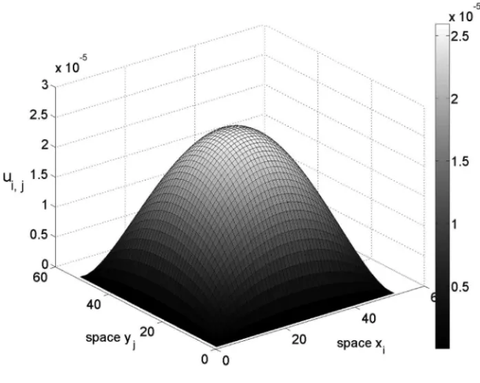
Our computational experiments were performed using MatLab consideringL1=L2=1,x=
y, where we have adopted two partitions with 50 divisions in each of the directionsxand y, the one that gave us a mesh with 2500 points. Below we present numerical simulations.
5.1 Discrete maximum principle simulations
The experiment shown here were obtained considering two separate cases. In the first case (Figures 1 and 2), the simulations were made usingqi,j = 7e−(2xi+3yi) and fi,j = −1. For
the second case (Figures 3 and 4), the simulations were made usingqi,j =7 sin(xi +3yi)and
fi,j =1.
Figure 1: Numerical solution.
Figure 3: Numerical solution.
RESUMO. Neste artigo tratamos as quest˜oes de convergˆencia, existˆencia e unicidade da
soluc¸˜ao num´erica de um problema el´ıptico discretizado pelo m´etodo de diferenc¸as finitas. A fim de provarmos a existˆencia e unicidade da soluc¸˜ao num´erica, usaremos uma configurac¸˜ao
variacional adequada (em n´ıvel discreto) para garantirmos a existˆencia de uma soluc¸˜ao
num´e-rica pelo m´etodo de diferenc¸as finitas.
Palavras-chave:equac¸˜oes el´ıpticas, diferenc¸as finitas, solvabilidade de soluc¸˜oes num´ericas.
REFERENCES
[1] H. Brezis. Functional Analysis, Sobolev Spaces and Partial Differential Equations, Universitext, Springer, (2010).
[2] L. Evans. Partial Differential Equations, Graduate Studies in Mathematics, American Mathematical Society,19(1998), 749 pp.
[3] D. Gilbarg & N.S. Trudinger. Elliptic Partial Differential Equations of Second Order, Classics in Mathematics, Springer, (2015).
[4] Q. Han & F. Lin. Elliptic Partial Differential Equations,Courant Lecture Notes in Mathematics, American Mathematical Society, (2011).
[5] K.W. Morton & D.F. Mayers. Numerical Solution of Partial Differential Equations: an Introduction,
Cambridge University Press, (2005).
[6] J.W. Thomas. Numerical Partial Differential Equations: Conservation Laws and Elliptic Equations,
Texts in Applied Mathematics, Springer, (1999).
[7] J.C. Strikwerda. Finite Difference Schemes and Partial Differential Equations, SIAM, (2004).
[8] W. Hackbusch. Elliptic Differential Equations: Theory and Numerical Treatment,Series in Compu-tational Mathematics. Springer,18(1992), 311 pp.