Additional Constraints to Ensure Three Vanishing Moments
for Orthonormal Wavelet Filter Banks and Transient Detection
J.C. UZINSKI1, H.M. PAIVA2, F. VILLARREAL3, M.A.Q. DUARTE4 and R.K.H. GALV ˜AO5
Received on November 26, 2013 / Accepted on February 4, 2015
ABSTRACT. This article presents an improvement to the formulation of Sherlock and Monro for the wavelet parameterization for the obtainment of the restrictions which ensure three vanishing moments. In order to test the formulation presented, a transient signal detection is presented.
Keywords:vanishing moments, additional constraints, transient detection.
1 INTRODUCTION
Sherlock and Monro [11] started the study of the angular parameterization of orthonormal filter banks, adapting the work of [14] on the factorization of paraunitary matrices and parameterizing the space of orthonormal wavelets by a set of angular parameters.
Initially the formulation had a weak point, there were no restrictions to ensure a number of vanishing moments greater than one. Additional constraints to ensure at least two vanishing moments were obtained by [9]. This article is an extension of [13] presenting an improvement to the formulation of [11]. In order to ensure a third vanishing moment for wavelet filter banks, additional constraints are presented to the work of [9] and [11]. An application of the formulation with three vanishing moments for transient detection is presented in this paper.
There are several works using the formulation proposed in [11] for several applications without the extensions to ensure more than one vanishing moment, for example, [1, 4, 5, 10]. However,
*Corresponding author: Julio Cezar Uzinski – E-mail: [email protected]
1Department of Electrical Engineering – FEIS, UNESP – Universidade Estadual Paulista, 15385-000 Ilha Solteira, SP, Brazil.
2Mectron – Organizac¸˜ao Odebrecht, 12227-000 S˜ao Jos´e dos Campos, SP, Brazil. E-mail: [email protected] 3Department of Mathematics – FEIS, UNESP – Universidade Estadual Paulista, 15385-000 Ilha Solteira, SP, Brazil. E-mail: [email protected]
4Department of Mathematics - UEMS, Universidade Estadual de Mato Grosso do Sul, 79540-000 Cassilˆandia, MS, Brazil. E-mail: [email protected]
after obtaining the constraints that ensure at least two vanishing moments, in [9], other papers have presented the use of that formulation and this restriction to various applications, some exam-ples are, [3, 8, 6]. The restriction achieved in this paper ensures at least three vanishing moments and was already applied to fault detection in [12], presenting promising results.
The remainder of the paper is organized as follows: in Section 2, formulas for assuring at least one and two vanishing moments are presented, in Section 3, the proposed formulation for a third vanishing moment is presented, Section 4 for presents an application to the proposed formulation, finally conclusions are presented in Section 5.
2 FIRST AND SECOND VANISHING MOMENTS
According to [11], let
H(N)(z)=
2N−1
i=0
h(iN)z−i, G(N)(z)=
2N−1
i=0
g(iN)z−i
be the transfer functions of the lowpass and highpass filters, respectively, for an orthonormal filter bank with length-2N, where
gi(N)=(−1)i+1h2(NN)−1−i, i =0,1, . . . ,2N−1, (2.1)
and
h(1)0 =cos(α1)
h(1)1 =sin(α1)
h(0N+1)=cos(αN+1)h(0N)
h(2Ni+1)=cos(αN+1)h(2Ni)−sin(αN+1)h(2Ni−)1
h(2NN+1)= −sin(αN+1)h(2NN)−1
h(1N+1)=sin(αN+1)h(0N)
h2(Ni++11)=sin(αN+1)h2(Ni)+cos(αN+1)h(2Ni−)1
h(2NN++1)1 =cos(αN+1)h(2NN)−1
i =0,1, . . . ,N−1. (2.2)
If the filter bank is to characterize a wavelet transform, the regularity conditionG(N)(z)|z=1=0 must be satisfied [2, 7]. Which, according to [9], leads to
αN=
π
4 −
N−1
i=1
αi, (2.3)
According to [7], to ensure two vanishing moments it is necessary that d G(d zN)(z)
z=1
=0.This
provides, [9],
αN−1 = 1 2arcsin
−1
2 −
N−2
i=1
sin
k
i=1 2αi
−
N−2
i=1
αi. (2.4)
Equation (2.4) has a real solution if the anglesαisatisfy the following condition
−3
2 ≤
N−2
i=1
sin
k
i=1 2αi
≤ 1
2. (2.5)
3 THE THIRD VANISHING MOMENT
In order to obtain a third vanishing moment, [13], it is necessary that
d2G(N)(z)
d z2
z=1
=0. (3.1)
Replacing (2.1) in the second derivative of G(N)(z)when z = 1 and writing conveniently, it becomes
d2G(N)(z)
d z2
z=1
= (N2+2N−1)
N−1
i=0
h(2Ni)
+
N−1
i=1
(2N +1)
⎡
⎣
N−1
i=0
h(2Ni)−2
N−1
i=N−j+1
h(2Ni)
⎤
⎦
+
N−2
j=1
N−j−1
k=1 2
⎡
⎣
N−1
i=0
h(2Ni)−2
k+j
i=k+1
h(2Ni)
⎤
⎦−(N2−1)
N−1
i=0
h(2Ni+)1
+
N−1
i=1
(2N −1)
⎡
⎣
N−1
i=0
h(2Ni+)1−2
N−1
i=N−j+1
h(2Ni+)1
⎤
⎦
−
N−2
j=1
N−j−1
k=1 2
⎡
⎣
N−1
i=0
h(2Ni+)1−2
k+j
i=k+1
h(2Ni+)1
⎤
⎦.
(3.2)
Lemma 3.1.Considering(2.2), the following equalities are true N−1
i=0
h(2Ni)=cos
N
i=1
αi
, (3.3)
N−1
i=0
h(2Ni+)1=sin
N
i=1
αi
Proof. Proof by induction:
In the case ofN =1, in (3.3) and (3.4), respectively, there are obtained the following values
h(1)0 =cos(α1) and h(1)1 =sin(α1).
Furthermore, it is necessary to demonstrate forN>1 that if
N−1
i=0
h(2Ni)=cos
N
i=1
αi
, (3.5)
N−1
i=0
h(2Ni−)1=sin
N
i=1
αi
(3.6)
then
N+1
i=0
h(2Ni+1) =cos
N+1
i=1
αi
, (3.7)
N+1
i=0
h(2Ni++11) =sin
N+1
i=1
αi
(3.8)
a) Demonstrate that the validity of (3.5) and (3.6) implies the validity of (3.7):
N+1
i=0
h(2Ni+1) =
N
i=0
cos(αN+1)h2(Ni)−sin(αN+1)h
(N) 2i−1
= cos(αN+1)
N
i=0
h(2Ni)−sin(αN+1)
N
i=0
h(2Ni−)1
= cos(αN+1)cos
N
i=1
αi
−sin(αN+1)sin
N
i=1
αi
= cos
αN+1+
N
i=1
αi
=cos
N+1
i=1
αi
b) Demonstrate that the validity of (3.5) and (3.6) implies the validity of (3.8):
N+1
i=0
h(2Ni++11) =
N
i=0
sin(αN+1)h(2Ni)+cos(αN+1)h(2Ni−)1
= sin(αN+1)
N
i=0
h(2Ni)+cos(αN+1)
N
i=0
h(2Ni−)1
= sin(αN+1)cos
N
i=1
αi
+cos(αN+1)sin
N
i=1
αi
= sin
(αN+1)+
N
i=1
αi
=sin
N+1
i=1
αi
Lemma 3.2.The equations in(2.2)imply
N−1
i=1
k
i=0
h(2Ni)−
N−1
i=0
h(2Ni)
=
N−1
i=1 cos
⎡
⎣
k
i=1
αi− N
i=k+1
αi
⎤
⎦, (3.9)
N−1
i=1
−
k
i=0
h(2N+)i+
N−1
i=0
h(2N+)i
=
N−1
i=1 sin
⎡
⎣
k
i=1
αi− N
i=k+1
αi
⎤
⎦. (3.10)
Proof. ForN =1 the verification of the validity of (3.9) and (3.10) is immediate.
ForN >1 show that if
N−1
i=1
⎡
⎣
k
i=0
h(2Ni)−
N−1
i=k+1
h(2Ni)
⎤
⎦=
N−1
i=1 cos
⎡
⎣
k
i=1
αi− N
i=k+1
αi
⎤
⎦ (3.11)
then
N+1
i=1
⎡
⎣
k
i=0
h(2Ni+1)−
N+1
i=k+1
h(2Ni+1)
⎤
⎦=
N+1
i=1 cos
⎡
⎣
k
i=1
αi− N+2
i=k+1
αi
⎤
⎦, (3.12)
and if
N−1
i=1
−
k
i=0
h(2N+)i+
N−1
i=0
h(2N+)i
=
N−1
i=1 sin
⎡
⎣
k
i=1
αi− N
i=k+1
αi
⎤
⎦ (3.13)
then
N+1
i=1
−
k
i=0
h(2N++i1)+
N+1
i=0
h(2N++i1)
=
N+1
i=1 sin
⎡
⎣
k
i=1
αi− N+2
i=k+1
αi
⎤
⎦. (3.14)
Demonstrate that the validity of (3.11) implies the validity of (3.12):
N+1
i=1
⎡
⎣
k
i=0
h(2Ni+1)−
N+1
i=k+1
h(2Ni+1)
⎤
⎦
=
N+1
i=1
k
i=0
cos(αN+1)h(2Ni)−sin(αN+1)h(2Ni−)1
−
N+1
i=k+1
cos(αN+1)h(2Ni)−sin(αN+1)h(2Ni−)1
⎤
⎦
=
N+1
i=1
cos(αN+1)
k
i=0
h(2Ni)−sin(αN+1)
k
i=0
h(2Ni−)1
−cos(αN+1)
N+1
i=k+1
h(2Ni)+sin(αN+1)
N+1
i=k+1
h(2Ni−)1
⎤
From Lemma 3.1 it follows that
N+1
i=1
⎡
⎣
k
i=0
h(2Ni+1)−
N+1
i=k+1
h(2Ni+1)
⎤
⎦
=
N+1
i=1
cos(αN+1)cos
k
i=0
αi −sin(αN+1)sin
k
i=0
αi
−cos(αN+1)cos
N+1
i=k+1
αi+sin(αN+1)sin
N+1
i=k+1
αi
⎤
⎦
=
N+1
i=1
⎡
⎣cos
αN+1+
k
i=0
αi
−cos
⎛
⎝αN+1+
N+1
i=k+1
αi ⎞ ⎠ ⎤ ⎦ =
N+1
i=1 cos
⎡
⎣
k
i=1
αi− N+2
i=k+1
αi
⎤
⎦.
Demonstrate that the validity of (3.13) implies the validity of (3.14):
N−1
i=1
−
k
i=0
h(2N+)i+
N−1
i=0
h(2N+)i
=
N−1
i=1
−
k
i=1
sin(αN+1)h(2Ni)+cos(αN+1)h(2Ni−)1
+
k
i=k+1
sin(αN+1)h(2Ni)+cos(αN+1)h(2Ni−)1
⎤
⎦
=
N−1
i=1
−sin(αN+1)
k
i=1
h(2Ni)−cos(αN+1)
k
i=1
h(2Ni−)1
+sin(αN+1)
k
i=k+1
h(2Ni)+cos(αN+1)
k
i=k+1
h(2Ni−)1
⎤
⎦.
From Lemma 3.1 it follows that
N−1
i=1
−
k
i=0
h(2N+)i+
N−1
i=0
h(2N+)i
=
N−1
i=1
−sin(αN+1)cos
k
i=0
αi−cos(αN+1)sin
k
i=0
αi
+sin(αN+1)cos
N+1
i=k+1
αi+cos(αN+1)sin
N+1
i=k+1
αi
⎤
=
N+1
i=1
−sin
αN+1+
k
i=1
αi
+sin
αN+1+
k
i=1
αi
=
N+1
i=1 sin
⎡
⎣
k
i=1
αi− N+2
i=k+1
αi
⎤
⎦.
From lemmas 3.1 and 3.2 it follows that (3.2) can be written as
d2G(N)(z)
d z2
z=1
= (N2+2N−1)cosβ−(N2−1)sinβ
+
N−1
j=1
(2N+1)cosβj +(2N−1)sinβj
+
N−2
j=1
N−j−1
k=1
2 cosβj,k−2 sinβj,k
(3.15)
where
⎧
⎪ ⎪ ⎪ ⎪ ⎪ ⎪ ⎪ ⎪ ⎪ ⎪ ⎪ ⎪ ⎪ ⎨
⎪ ⎪ ⎪ ⎪ ⎪ ⎪ ⎪ ⎪ ⎪ ⎪ ⎪ ⎪ ⎪ ⎩
β =
N
i=1
αi
βj = N
i=1
αi−2 N
i=(N−j)+1
αi, 1≤ j≤ N−1
βj,k = N
i=1
αi−2 k+j
i=k+1
αi, 1≤ j≤ N−1 and 1≤k≤N −1.
(3.16)
From equation (2.3), equation (3.16) has the following implications:
β =π
4, βj =
π
4 −2
N
i=(N−j)+1
αi and βj,k=
π
4 −2
k+j
i=k+1
αi.
Leading to some properties:
(N2+2N−1)cosβ−(N2−1)sinβ =2Ncosπ 4,
cos
⎡
⎣
π
4 −2
N
i=(N−j)+1
αi
⎤
⎦+sin
⎡
⎣
π
4 −2
N
i=(N−j)+1
αi
⎤
⎦
=2 cosπ 4 cos
⎡
⎣2
N
i=(N−j)+1
αi
⎤
cos
⎡
⎣
π
4 −2
k+j
i=k+1
αi
⎤
⎦−sin
⎡
⎣
π
4 −2
k+j
i=k+1
αi
⎤
⎦=2 cos
π
4 sin
⎡
⎣2
k+j
i=k+1
αi ⎤ ⎦, cos ⎡ ⎣ π
4 −2
N
i=(N−j)+1
αi
⎤
⎦=cos
π 4 ⎛ ⎝cos ⎡ ⎣2 N
i=(N−j)+1
αi
⎤
⎦+sin
⎡
⎣2
N
i=(N−j)+1
αi
⎤
⎦ ⎞
⎠.
Using such properties, equations (3.15-3.16) can be written as:
d2G(N)(z)
d z2
z=1
= 2Ncosπ
4 +
N−1
j=1
2 cosπ
4(cosλj+sinλj)+2(2N−1)cos
π
4 cosλj
(3.17)
+
N−2
j=1
N−j−1
k=1
4 cosπ 4 sinλk
whereλj =
⎡
⎣2
N
i=(N−j)+1
αi
⎤
⎦andλk =
⎡
⎣2
k+j
i=k+1
αi
⎤
⎦.
Applying (3.1) in (3.17)
0 = N+
N−1
j=1
sinλj+2Ncosλj
+
N−2
j=1
N−j−1
k=1
(2 sinλk)
, (3.18)
Then (3.18) should be written in terms ofαN−2, firstly rewriting (3.18),
N−1
j=1
sinλj+2Ncosλj
+
N−2
j=1
N−j−1
k=1 2 sin
⎡
⎣
k+j
i=k+1 2αi
⎤
⎦
+N =0. (3.19)
Decomposing the second parcel of (3.19) gives
N−1
j=1
sinλj+2Ncosλj
+2 sin
N−1
2 2αi
+
N−3
j=1
N−j−1
k=1 2 sin
⎡
⎣
k+j
i=k+1 2αi
⎤
⎦
= −N
and following the reasoning
2 sin
N−1
2 2αi
= − ⎧
⎨
⎩
N−1
j=1
sinλj +2Ncosλj
+
N−3
j=1
N−j−1
k=1
2 sinλk
+N
⎫
⎬
N−1
2
2αi =arcsin
⎧
⎨
⎩ −
N−1
j=1
1
2sinλj +Ncosλj
−
N−3
j=1
N−j−1
k=1 sinλk
− N
2
⎫
⎬
⎭
N−1
i=2,i=N−2
2αi+2αN−2=arcsin
⎧
⎨
⎩ −
N−1
j=1
1
2sinλj+Ncosλj
−
N−3
j=1
N−j−1
k=1 sinλk
− N
2
⎫
⎬
⎭
αN−2= 1 2arcsin
⎧
⎨
⎩ −
N−1
j=1
1
2sinλj+Ncosλj
−
N−3
j=1
N−j−1
k=1 sinλk
− N
2
⎫
⎬
⎭ −
N−1
i=2,i=N−2
αi.
(3.20)
Equation (3.20) ensures the third vanishing moment, and it has a real solution if the anglesαi
satisfy the condition
−1−N
2 ≤
⎧
⎨
⎩
N−1
j=1
1
2sinλj+Ncosλj
+
N−3
j=1
N−j−1
k=1 sinλk
⎫
⎬
⎭
≤1− N
2. (3.21)
4 TRANSIENT DETECTION IN A SIGNAL
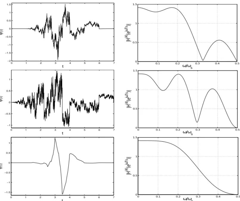
Consider a orthonormal filter bank with length-8 (N = 4), which initial configuration charac-terizes a wavelet with at least one vanishing moment, αp=1 = {−17.38◦, 16.83◦,−45.10◦, 90.65◦}. In order to ensure two vanishing moments complies (2.4) must be used resulting in
αp=2= {−17.38◦,16.83◦,3.12◦,42.43◦}. In order to ensure at least three vanishing moments apply (3.20) which leads toαp=3= {−17.38◦,−47.23◦,93.44◦,16.17◦}. Figure 1 shows the functionsψ (t): αp=1,αp=2andαp=3, respectively. Each wavelet has the sampling frequency
which is denoted byωs =2π/T s.
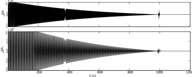
Let f(t)be the signal shown in Figure 2,
f(t)= ⎧
⎪ ⎪ ⎪ ⎪ ⎪ ⎨
⎪ ⎪ ⎪ ⎪ ⎪ ⎩
t
et if 0≤t <377,
(t−0.001)
et if 377≤t <995,
0 1 2 3 4 5 6 7
−1.5
−1
−0.5
0 0.5 1
t
ψ
(t)
0 1 2 3 4 5 6 7
−1
−0.5
0 0.5 1
t
ψ
(t)
0 1 2 3 4 5 6 7
−2
−1.5
−1
−0.5
0 0.5 1 1.5
t
ψ
(t)
0 0.1 0.2 0.3 0.4 0.5
0 0.5 1 1.5
/s
|H
(4
) (e
j
Ts )|
0 0.1 0.2 0.3 0.4 0.5
0 0.5 1 1.5
/s
|H
(4
) (e
j
Ts )|
0 0.1 0.2 0.3 0.4 0.5
0 0.5 1 1.5
/s
|H
(4
) (e
j
Ts )|
Figure 1: On the left: αp=1, αp=2andαp=3. On the right: the sampling frequency of each
wavelet.
Figure 2: Signal f(t).
This signal has two transients (discontinuities), whent = 377s andt = 995s, and it was an-alyzed usingαp=1, αp=2and αp=3, according to Figures 3, 4 and 5. Each figure shows the
1 0 1x 10
3
d
1200 400 600 800 1000 1200
2 1 0 1 2x 10
3
d
2t (s)
Figure 3: Analysis of f(t)withαp=1in the first and second level of decomposition.
200 400 600 800 1000 1200
1 0 1x 10
3
d
2t (s) 1
0 1x 10
3
d
1Figure 4: Analysis of f(t)withαp=2in the first and second level of decomposition.
1 0 1x 10
3
d
1200 400 600 800 1000 1200
1 0 1x 10
3
d
2t (s)
Figure 5: Analysis of f(t)withαp=3in the first and second level of decomposition.
Comparing Figures 3, 4 and 5 it is noticed that in spite of the good identification of transients usingαp=2, the analysis withαp=3also provides a good result. But forαp=1, the detection is not
coefficients indicates that the transients are slightly more highlighted when the analysis is done usingαp=3.
There are other formulations to work with wavelet filter banks, for example, [15], but the for-mulation of Sherlock and Monro stands for the mathematical and computational simplicities. However, initially there were no constraints to ensure a number of vanishing moments greater than one. An extension of this formulation introducing restrictions to ensure two vanishing mo-ments was done by [9]. In [13] the constraints to ensure at least three vanishing momo-ments were presented.
Several papers on applications using this formulation before the extension for three vanishing moments have been published, some examples are, such as pattern recognition [4], linear esti-mation [5], and signal compression [10].
5 CONCLUSIONS
This paper presented the constraints that ensure three vanishing moments and also demonstra-tions and calculademonstra-tions for the obtaining. It also presents a brief application of the formulation for transient detection in signals, a comparative way between wavelets with different regularities.
In this paper, an application example was used to test the three different wavelets of Sherlock and Monro. Through this example it was noticed that those wavelets are efficient in transient detection, specially when regularity is of at least two vanishing moments. In the case that the parameterization satisfies at least three vanishing moments it was obtained a good identification of transients and better compression or the regular parts of the signal. This fact supports the idea that the more regular is the wavelet the better is the compression of the regular parts of the signal to be decomposed.
ACKNOWLEDGMENTS
The authors would like to thank the Brazilian agencies FAPESP (grant 2011/17610-0) and CNPq (research fellowships and PhD grant 160545/2013-7).
RESUMO.Este artigo apresenta uma melhoria para a formulac¸˜ao de Sherlock e Monro para a parametrizac¸˜ao wavelet para a obtenc¸˜ao das restric¸ ˜oes que garantem trˆes momentos nulos. A fim de testar a formulac¸˜ao apresentada, um exemplo de detecc¸˜ao de transit´orios em sinais ´e apresentada.
Palavras-chave:Momentos nulos, restric¸ ˜oes adicionais, detecc¸˜ao de transit´orios.
REFERENCES
[1] A. Daamouche & F. Melgani. Swarm Intelligence Approach to Wavelet Design for Hyperspectral Image Classification,Geoscience and Remote Sensing Letters, IEEE,6(4), pp. 825–829, Oct. 2009.
[3] M.A.Q Duarte, R.K.H. Kawakami & H.M. Paiva. Bi-objective optimization in a wavelet identification procedure for fault detection in dynamic systems,Industrial Electronics and Applications (ICIEA), 2013 8th IEEE Conference on, pp. 1319–1324, June 2013.
[4] T. Froese, S. Hadjiloucas, R.K.H. Galv˜ao, V.M. Becerra & C.J. Coelho. Comparison of extrasystolic ECG signal classifiers using discrete wavelet transforms,Pattern Recognit. Lett., 27, pp. 393–407, Apr. 2006.
[5] R.K.H. Galv˜ao, G.E. Jos´e, H.A.D. Filho, M.C.U. Araujo, E.C. Silva, H.M. Paiva, T.C.B. Saldanha & E.S.O.N. Souza. Optimal wavelet filter construction using X and Y data,Chemometrics and Intelli-gent Laboratory Systems,70, pp. 1–10, Jan. 2004.
[6] S. Hadjiloucas, N. Jannah, F. Hwang & R.K.H. Galv˜ao. On the application of optimal wavelet filter banks for ECG signal classification,Journal of Physics: Conference Series,490(2014).
[7] S. Mallat. “A Wavelet Tour of Signal Processing”. San Diego, EUA: Academic Press, (1998).
[8] H.M. Paiva & R.K.H. Galv˜ao. Optimized orthonormal wavelet filters with improved frequency sepa-ration. Digital Signal Processing,22(4), pp. 622–627, July 2012.
[9] H.M. Paiva, M.N. Martins, R.K.H. Galvao & J. Paiva. On the space of orthonormal wavelets: addi-tional constraints to ensure two vanishing moments,Signal Processing Letters, IEEE,16(2), pp. 101– 104, Feb. 2009.
[10] J.P.L.M. Paiva, C.A. Kelencz, H.M. Paiva, R.K.H. Galv˜ao & M. Magini. Adaptive wavelet EMG compression based on local optimization of filter banks.Physiological Measurement,29(2008), 843– 856.
[11] B.G. Sherlock & D.M. Monro. On the space of orthonormal wavelets.Signal Processing, IEEE Trans-actions on,46(6), pp. 1716–1720, June 1998.
[12] J.C. Uzinski. Vanishing moments and wavelet regularity in the fault detection of signals (in Por-tuguese), (M.Sc. thesis) Ilha Solteira, SP, Brazil, (2013).
[13] J.C. Uzinski, H.M. Paiva, F. Villarreal, M.A.Q. Duarte & R.K.H. Galv˜ao. Additional constraints to ensure three vanishing moments for orthonormal wavelet filter banks, Congresso de matem´atica aplicada e computacional – Centro-Oeste, Cuiab´a – MT, July 2013.
[14] P.P. Vaidyanathan. “Multirate Systems and Filter Banks”. Englewood Cliffs, NJ: Prentice-Hall, 1993.