Closed-Form Solution for the Solow Model with Constant Migration
J.P. JUCHEM NETO1*, J.C.R. CLAEYSSEN2, D. RITELLI3 and G. MINGARI SCARPELLO4
Received on May 17, 2014 / Accepted on March 26, 2015
ABSTRACT.In this work we deal with the Solow economic growth model, when the labor force is ruled by the Malthusian law added by a constant migration rate. Considering a Cobb-Douglas production function, we prove some stability issues and find a closed-form solution for the emigration case, involving Gauss’ Hypergeometric functions. In addition, we prove that, depending on the value of the emigration rate, the economy could collapse, stabilize at a constant level, or grow more slowly than the standard Solow model. Immigration also can be analyzed by the model if the Malthusian manpower is declining.
Keywords:Solow growth model, migration, hypergeometric function.
1 INTRODUCTION
The Solow one-sector model for economic growth [10], [11] is a landmark in the neoclassic theory of growth, which originated an enormous literature. One of the main assumptions of this model is the labor force ruled by a Malthusian Law, namely an exponential population growth. Joining to this a Cobb-Douglas production function, this model has a well known analytical so-lution. Relatively recent works have replaced the Malthusian Law by other population growth models. Donghan [5] proposed the replacement by the Verhulst (logistic) Law in the Solow model, without actually solving it, but proving the reaching of a steady state. In the same paper, he proves a comparison, a limit and a stability theorem for the capital per capita evolution, under the assumption of a strictly increasing and bounded labor force. In [9] Mingari Scarpello and Ritelli have shown that for the case of the Verhulst (logistic) Law, the model admits a closed-form solution in terms of the Gauss’ Hypergeometric function2F1. After that, in [4] the Von
*Corresponding author: Jo˜ao Pl´ınio Juchem Neto
1Centro de Tecnologia de Alegrete, UNIPAMPA – Universidade Federal do Pampa, 97546-550 Alegrete, RS, Brasil. E-mail: [email protected]
2Instituto de Matem´atica, UFRGS – Universidade Federal do Rio Grande do Sul, 91509-900 Porto Alegre, RS, Brasil. E-mail: [email protected]
3Dipartimento di Scienze Statistiche, Universit`a di Bologna, Via Belle Arti 41, Bologna, Italy. E-mail: [email protected]
Bertalanffy Law was considered arriving at a closed-form solution involving2F1, and in [1] was
introduced the Richards Law (a generalized logistic model). In our paper we talk about “migra-tions” meaning the impact of a constant additional manpower I to the classic Malthusian law which feeds the Solow model. We show that this model also has a closed-form solution in terms of the function2F1, forI < 0 (labor force emigration). This kind of model can be applied to
study the brain drain phenomena [7], for example. In the following section we review the classic Solow Model, and in Section 3 we present the model modified by the migration term, discuss the stability and steady-state of the capital and output per capita, and solve it. In Section 4 we discuss briefly the case in which we have immigration (I >0), and in Section 5 we present some simulations. Finally, in Section 6 we state our conclusions.
2 THE SOLOW MODEL FOR ECONOMIC GROWTH
The Solow growth model [10] assumes a production function f depending on the accumulated stock of capitalK(t)and labor forceL(t)at a timet, and on a constant factorA, a given param-eter representing the technological level of the economy:
Y = f(K,L,A), withK,L,A>0 (2.1)
This production function must meet the following properties:
i) f(·)is an increasing function in both state variables, capital and labor force
∂f
∂K >0, ∂f ∂L >0
, with decreasing marginal returns
∂2f ∂K2 <0,
∂2f ∂L2 <0
.
ii) f(·)shall have constant returns to scale, f(λK, λL)=λf(K,L),∀λ >0.
iii) f(·)satisfies theInada conditions:
lim
K→0 ∂f
∂K =Llim→0 ∂f
∂L = +∞ and K→+∞lim ∂f
∂K =L→+∞lim ∂f ∂L =0.
One of the production function satisfying conditions i, ii and iii, used by Solow in his seminal work was the Cobb-Douglas function giving the outputY as:
Y =AKϕL1−ϕ, withϕ ∈(0,1) (2.2)
whereϕ closer to 0 means a labor intensive economy, andϕcloser to 1 a capital intensive one. Considering (2.2), the capital stock dynamics is ruled by the ordinary differential equation:
˙
K =sY−δK =s AKϕL1−ϕ−δK (2.3)
wheres andδ are the constant saving and depreciation rates, thensY is the gross investment, andδK is the capital depreciation in the whole economy. The labor force dynamics follows the Malthusian Law:
˙
withL0>0 being the initial population of workers. Defining the capital per capita:
k(t)= K(t)
L(t) (2.5)
and the labor force growth rate:
n(t)= ˙ L(t)
L(t) (2.6)
and taking (2.4) into account, we rewrite (2.2) and (2.3) as:
Y = AL(t)kϕ(t) (2.7)
Y =AL0eαtkϕ, withϕ∈(0,1) (2.8) ˙
k+(n(t)+δ)k=s Akϕ (2.9)
Then, noting from (2.4) and (2.6) thatn(t) = α, the solution of the Bernoulli equation (2.9), given the initial capital per capitak(0)=k0>0 is:
k(t)=
As
1−e−t(1−ϕ)(α+δ)
+k01−ϕ(α+δ)e−t(1−ϕ)(α+δ) α+δ
1 1−ϕ
(2.10)
and the total output is given plugging (2.10) in (2.8). Observe that the steady-state of the capital per capita,k∞, is given by:
k∞= lim
t→+∞k(t)=
s A α+δ
1−1ϕ
. (2.11)
Defining the output per capita
y(t)= Y(t) L(t)= Ak
ϕ(t) (2.12)
where we used (2.7), such output, in the long run, will tend to:
y∞= lim
t→+∞Ak
ϕ(t)= A
s A
α+δ 1−ϕϕ
. (2.13)
3 THE SOLOW GROWTH MODEL WITH MIGRATION
In this work we will add a constant migration rateI in the r.h.s. of the differential equation (2.4) that governs the growth of the labor force:
˙
L =αL+I (3.1)
whose solution is:
L(t)= −I α+
L0+
I α
Observe that, making I = 0, we recover the exponential law (2.4), and besides of that limt→+∞n¯(t) = α (the over score will mark hereinafter all the ratios relevant to migration
model) where, in this case:
¯
n(t)= L˙(t) L(t)=
α(αL0+I) αL0+I1−e−αt
(3.3)
That is, in the long run, the variation rate of the labor force tends to the same valueαof the ex-ponential law. In principle, the migration rate I (number of individuals per time) is an exogenous variable that could be positive (immigration, workers entering the labor force at a constant rate), negative (emigration, workers leaving the labor force) or zero (no migration). Then, considering (3.3) and the change of variable
z= ¯k1−ϕ (3.4)
we can rewrite (2.9) as the following linear differential equation, now inz(t):
˙
z−(ϕ−1)(δ+ ¯n(t))z =(1−ϕ)s A (3.5)
subject to the initial conditionz(0)=z0=k10−ϕ. Defining the integrating factor:
H(t)=(ϕ−1)
t
0
(δ+ ¯n(τ ))dτ =(ϕ−1)δt+(ϕ−1)ln
L(t)
L0
(3.6)
then the solution of (3.5) is given by:
z(t)=z0eH(t)+(1−ϕ)s At eH(t)
t
0
e−H(τ )dτ. (3.7)
3.1 Stability and Steady-State
Before starting to formulate an analytical expression for (3.7), and therefore for k¯(t), let us discuss the stability and asymptotes ofk¯(t), consideringα, L0>0.
Proposition 1.
i) The capital per capitak¯(t)is globally asymptotically stable for I ∈ [−αL0,0].
ii) The capital per capita goes to infinity within a finite time if I ∈ (−∞,−αL0), that is, limt→t∗k¯(t)= +∞where t∗= 1
αln
I
αL0+I
.
Proof.
thatk¯(t)is also globally asymptotically stable. First, let us consider a solutionv(t)of (3.5) subjected to the arbitrary positive initial conditionv(0)=v0 >0. This solution is given by:
v(t)=v0eH(t)+(1−ϕ)s At eH(t)
t
0
e−H(τ )dτ. (3.8)
Considering (3.7) and (3.8), we have that|z(t)−v(t)| = |z0−v0|eH(t). By (3.2), and
for I ∈ [−αL0,0], we have that L(t) → +∞ast → +∞. Besides of that, because ϕ ∈ (0,1), limt→+∞H(t)= −∞by (3.6). Therefore: limt→+∞|z(t)−v(t)| =0 and
then, we infer the global asymptotic stability ofz(t)andk¯(t).
ii) IfI ∈(−∞,−αL0), we have thatL(t∗)=0 for a finite timet∗given by
t∗= 1 αln
I
αL0+I
.
This implies that limt→t∗H(t) = +∞, and by (3.7), that limt→t∗z(t) = +∞. Then,
t =t∗is a vertical asymptote for bothz(t)andk¯(t).
Proposition 2.The steady-state capital per capitak¯∞is given by:
i) k¯∞=
s A
δ+α 1−1ϕ
, if I∈(−αL0,0].
ii) k¯∞=s Aδ
1
1−ϕ, if I = −αL 0.
Proof. First, observe that we can find the horizontal asymptote z∞ for z(t) making ˙z =
0 in the differential equation (3.5), isolating z(t), and taking its limit as t → +∞, z∞ =
limt→+∞δ+ ¯s An(t), wheren¯(t)is given by (3.3). Therefore, by (3.4),k¯∞can be written as:
¯ k∞=
s A
δ+limt→+∞n¯(t) 1−1ϕ
. (3.9)
i) ForI ∈(−αL0,0], we have that limt→+∞n¯(t)=αby (3.3), and thenk¯∞=
s A
δ+α 1−1ϕ
.
ii) IfI = −αL0, the labor force remains constant over time, and again by (3.3),n¯(t)≡ 0.
Thereforek¯∞=s Aδ
1 1−ϕ.
Using (2.12), and the above results, we get the propositions below, involving the output per capita
¯ y(t).
Proposition 3.
ii) The output per capita goes to infinity at a finite time if I ∈ (−∞,−αL0), that is,
limt→t∗y¯(t)= +∞where t∗= 1
α ln
I
αL0+I
.
Proposition 4.The steady-state output per capitay¯∞is given by:
i) y¯∞=A
s A
δ+α 1−ϕϕ
, if I ∈(−αL0,0].
ii) y¯∞=As Aδ ϕ
1−ϕ, if I = −αL 0.
Note that the labor force emigration critical value capable of offsetting the population growth is I = −αL0, maintaining the labor force constant. In this case, by Propositions 2(ii) and 4(ii), we have that the level of capital and output per capita in the long-run are greater than in the case without emigration (2.11) and (2.13):
¯ k∞=
s A
δ 1−1ϕ
>
s A
δ+α 1−1ϕ
=k∞
¯ y∞=A
s A
δ 1−ϕϕ
>A
s A
δ+α 1−ϕϕ
=y∞
(3.10)
becauseα >0. Otherwise, if I ∈ (−αL0,0], we can see, by Propositions 2(i) and 4(i), that the equality holds, i.e.:
¯
k∞=k∞andy¯∞=y∞ (3.11)
Then it is clear the criticality of the emigration threshold I = −αL0: below it bothk¯∞andy¯∞ are greater than the correspondent classic values, while above it, they equate the classic ones.
3.2 Closed-form Solution forI <0
Integrating (3.7) and coming back tok¯(t), we find that:
¯ k(t)=
eH(t)
¯
k10−ϕ+(1−ϕ)s A
t
0
e−H(τ )dτ 1−1ϕ
(3.12)
where by (3.6):
H(t)=(ϕ−1) t
0
(δ+ ¯n(τ ))dτ =(ϕ−1)δt+ln
eαt
1+ I αL0
− I
αL0 ϕ−1
The integral in (3.12) is given by:
ᑣ=
t
0
e−H(τ )dτ = t
0
e(1−ϕ)δτ
eατ
1+ I αL0
− I
αL0 1−ϕ
dτ
Following [9] we carry out the change of variableu =eατ:
ᑣ = 1
α eαt
1
u(1−αϕ)δ−1
− I
αL0 +
1+ I αL0
u
= 1 α
− I
αL0
1−ϕ eαt
1
u(1−αϕ)δ−1
1−
1+αL0 I
u
1−ϕ du
where in the last step we have to consider I < 0, in order to guarantee a real value to the
expression−αLI
0
1−ϕ .
The last integral relates to the Euler’s integral representation of the Gauss’ Hypergeometric Func-tion2F1(see [2], [6], [8]):
2F1 a,b
c x = ∞
n=0
(a)n(b)n
(c)n
zn
n!
= Ŵ(c)
Ŵ(c−b)Ŵ(b)
1
0
tb−1(1−t)c−b−1(1−zt)−adt
where(.)nis a Pochhammer symbol. The series is convergent for anya, b, cif|z|<1, and for
Re{a+b−c}<0 if|z| =1. For the integral representation is requiredRe(c) > Re(b) >0. HereŴ(z)denotes the Gamma Function. A quick overview of Gauss’ Hypergeometric Function can be found in [3].
After some algebra, we can write the integralᑣin the closed-form
ᑣ= 1
α
− I
αL0 1−ϕ
(ᑣt−ᑣ0) (3.13)
where:
ᑣ0= α
(1−ϕ)δ 2F1 a,b
c z1 (3.14)
ᑣt =αe
(1−ϕ)δt
(1−ϕ)δ 2F1 a,b
c z2 (3.15)
anda, b, c, z1, z2are defined as:
a=ϕ−1, b =(1−ϕ)δ α , c=
(1−ϕ)δ α +1
z1=1+ αL0
I , z2=
1+αL0 I
eαt
(3.16)
Finally, the capital per capita (3.12) is given by:
¯ k(t)=
e(ϕ−1)δt
eαt
1+ I αL0
− I
αL0 ϕ−1
×
¯
k01−ϕ+s(1−ϕ)A α
− I
αL0 1−ϕ
(ᑣt −ᑣ0)
1 1−ϕ
whereI <0,ϕ ∈(0,1),L0, α,s, δ >0 andᑣ0,ᑣt are given by (3.14)-(3.16). Plugging (3.2)
and (3.17) in (2.7) we get the gross output of the economy:
¯
Y(t)= A α
(αL0+I)eαt −Ik¯(t)ϕ (3.18)
which describes the total production of the economy when the natural Malthusian labor force growth is modified by a constant emigration rate of workers. This framework could be used in the analysis of brain drain phenomena, for instance. Observe that if the emigration rate is too strong (I <−αL0), the economy collapses at a finite time; if the emigration is equal to minus
the initial labor force rate, the total output converges to−I Aα s A
δ
1−ϕϕ; and if−αL
0 < I <0
we have an output always minor than in the absence of emigration. As we will see in the next section, (3.18) is also valid in a scenario where there is immigration, but in a declining labor force environmental, that nowadays is a realistic one in some developed countries.
4 WHAT ABOUT IMMIGRATION?
Due to the structure of our described growth model, a transient including immigration cannot be treated: in fact with I > 0 and α > 0, (3.1) gives an exponential manpower, L(t) =
1 α
(αL0+I)eαt−I, growing during time well faster than the MalthusianL0eαt. In such a
way there would exist a finite instant defined byt∗=α1lnαL0I+Iat which by (3.3) the coeffi-cientn¯(t)in (3.5) becomes infinite, so that all the microeconomic model would burst out. Thus for a positive trendα >0 no situationI >0 is possible, unlesst <t∗.
This can be seen also through (3.17) in which the reality ofα−L0I
1−ϕ
requiresαandI to be opposite in sign. Then an immigration(I >0)could be in principle “balanced” by a negative trend(α <0)of the Malthus manpower law. In this case the polet∗will be negative for an initial population such that the addition of the immigration rate to the initial labor force rate is positive. Otherwise the pole ofn¯(t)would be innoxius and not real.
The sense of all this is that an exogenous contribution of manpower can be absorbed by the system whenever its labor force is declining. Otherwise in presence of a (also slightly) own growing labor force, whichever immigration will push the system sooner or later beyond its capabilities and then will cause its explosion.
It is straightforward to show that ifα < 0 and I > 0, then the capital and output per capita steady-states are given by
¯ k∞=
s A
δ 1−1ϕ
<
s A
δ+α 1−1ϕ
=k∞ (4.1)
¯ y∞= A
s A
δ 1−ϕϕ
< A
s A
δ+α 1−1ϕ
=k∞ (4.2)
As a last remark, observe that in the case of a decaying manpower Malthusian Law, the total output steaty-stateY∞is zero. But when we balance it with a positive migration rate (I >0), we
have that:
¯ Y∞= −
I A α
s A
δ 1−ϕϕ
>0=Y∞ (4.3)
5 SAMPLE PROBLEMS
Considering the set of parametersα = 0.02, ϕ = 0.5, δ = 0.05, s = 0.06, A =1, k¯0 =
200, L0 =100, we plotted the gross output of the economy given by (3.18) in Figure 1. Note
that: whenI = −αL0 = −2, the labor force emigration compensates the population growth,
implying a constant labor force, and the convergence of the total outputY¯(t)of the economy to a constant value in the long run, ast → +∞; when I ∈ (−αL0,0)=(−2,0), as a result of emigration, the labor force grows more slowly than in the classic Solow model, which causes a slow increase in the total outputY¯(t); if I = 0, we have no emigration, andY¯(t)grows in an exponential way, given by classic Solow model; if I ∈ (−∞,−αL0) = (−∞,−2), the emigration rate is greater than the natural growth rate of the labor force, causing its extinction. In this case,Y¯(t)becomes zero at a finite timet∗, leading the economy to a collapse.
0 50 100 150 200 250 300
10−1 100 101 102 103 104 105
t
Y(t)
I= 0.00 I=−1.00 I=−1.90 I=−2.00 I=−2.01 I=−2.10
Observe that in this last case, from the proof of Proposition 1(i), the timet∗at which the economy collapses is given by:
t∗= 1 αln
I
αL0+I
(5.1)
whenL(t∗)=0, and thenY(t∗)=0, from (3.18).
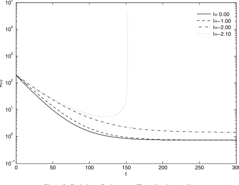
In Figure 2 we show the capital per capita evolution, for some values ofI: whenI = −αL0= −2, the capital per capita get steady at an upper level than the Solow model, when I =0 (see result (3.10)); when I = −1 ∈ (−αL0,0)= (−2,0),k¯(t)in the short term are greater when there is emigration, than when there is not, but whent → +∞, it tends to the same level given by the Solow model (see result (3.11)); ifI →0−, we recover the behaviour of the classic Solow model; if I = −2.1 ∈ (−∞,−αL0)=(−∞,−2), L(t)=0 in a finite timet∗, which implies thatk¯(t)→ +∞ast→t∗, but remember that in this case we have the collapse of the economy, withY¯(t∗)=0, as noted in Figure 1 (see Proposition 1(ii)).
0 50 100 150 200 250 300
10−1 100 101 102 103 104 105
t
k(t)
I= 0.00 I=−1.00 I=−2.00 I=−2.10
Figure 2: Capital per CapitaversusTime (I <0, α >0).
0 50 100 150 200 250 300 103
104 105
t
Y(t)
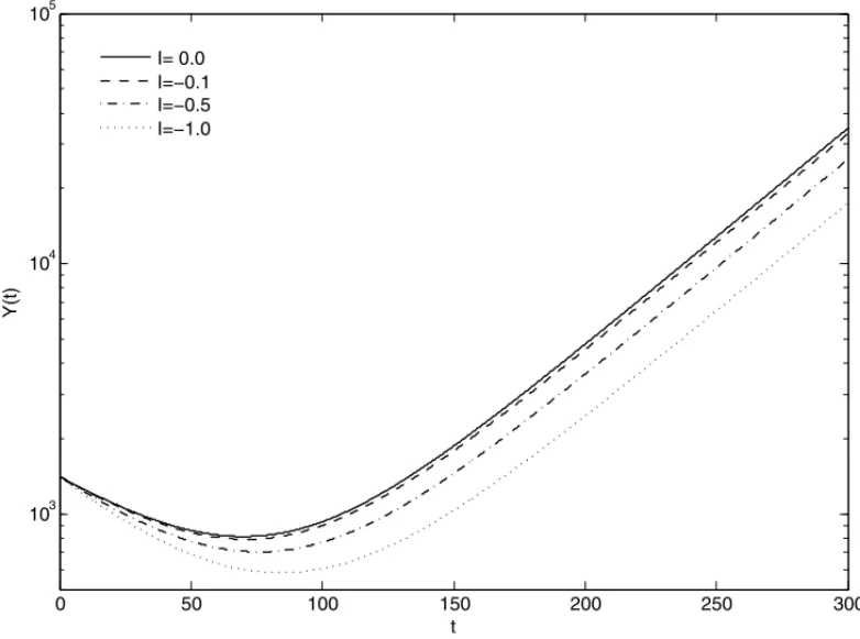
I= 0.0 I=−0.1 I=−0.5 I=−1.0
Figure 3: Gross output versus time and its convergence to the classic model as I → 0− (I <0, α >0).
6 CONCLUSIONS
In this paper we derived a closed-form solution for the Solow growth model involving the Gauss’ Hypergeometric Function2F1, assuming the dynamics of the labor force to follow a Malthusian
Law with a constant emigration rate I <0, such that when I → 0−the classic Solow model is recovered. We also proved the global asymptotic stability of the capital and output per capita for I ∈ [−αL0,0], although the closed-form solution presented is only valid in the interval I ∈ [−αL0,0). Besides of that, our analytical simulations for a specified set of parameters prove that the range of emigrationI ∈ (−∞,−αL0)is such that the labor force becomes zero at a finite time, leading the economy to a collapse. For I = −αL0the labor force keeps constant,
0 100 200 300 400 500 600 700 800
10−5 10−4 10−3 10−2 10−1 100 101 102 103 104
t
Y(t)
I=0.0000 I=0.0001 I=0.0010 I=1.0000 I=10.000 I=100.00
Figure 4: Gross OutputversusTime (I >0, α <0).
0 100 200 300 400 500 600 700 800
100 101 102 103
t
k(t)
I=0.0000 I=0.0001 I=0.0010 I=1.0000 I=10.000 I=100.00
RESUMO. Neste trabalho consideramos o modelo de crescimento econˆomico de Solow,
quando a forc¸a de trabalho ´e governada pela lei de Malthus adicionada por uma taxa de migrac¸˜ao constante. Considerando a func¸˜ao de produc¸˜ao de Cobb-Douglas, provamos alguns
resultados de estabilidade e encontramos uma soluc¸˜ao em forma fechada, envolvendo func¸˜oes
hipergeom´etricas de Gauss, para o caso em que h´a emigrac¸˜ao. Al´em disso, provamos que, dependendo do valor da taxa de emigrac¸˜ao, a economia pode entrar em colapso, estabilizar
em um n´ıvel constante, ou crescer mais vagarosamente do que o modelo de Solow padr˜ao.
O caso em que h´a imigrac¸˜ao tamb´em pode ser analisado pelo modelo, desde que a taxa de crescimento orgˆanico de trabalhadores na Lei de Malthus seja negativa.
Palavras-chave:Modelo de crescimento de Solow, migrac¸˜ao, func¸˜ao hipergeom´etrica.
REFERENCES
[1] E. Accinelli & J.G. Brida. Re-formulation of the Solow economic growth model whit the Richards population growth law. GE, Growth, Math methods 0508006, EconWPA, 2005. Available in: http://ideas.repec.org/p/wpa/wuwpge/0508006.html.
[2] G.E. Andrews, R. Askey & R. Roy.Special Functions, Cambrigde Press (1999).
[3] R. Boucekkine & J.R. Ruiz-Tamarit. Special functions for the study of economic dynamics: The case of the Lucas-Uzawa model.Journal of Mathematical Economics,44(2008), 33–54.
[4] J.G. Brida & E.J.L. Maldonado. Closed form solutions to a generalization of the Solow growth model. Applied Mathematical Sciences,1(40) (2007), 1991–2000.
[5] C. Donghan. An Improved Solow Model.Chinese Quarterly Journal of Mathematics,13(2) (1998), 72–78.
[6] A. Erd´elyi (Editor). Higher Transcendental Functions – Volume I, McGraw-Hill Book Company, USA, (1953).
[7] P. Pieretti & B. Zou. Brain drain and factor complementarity.Economic Modelling (2008), doi: 10.1016/j.econmod.2008.08.002.
[8] E.D. Rainville.Special Functions. The Macmillian Company, New York (1960).
[9] G. Mingari Scarpello & D. Ritelli. The Solow Model Improved Through the Logistic Manpower Growth Law.Annali Universit`a di Ferrara – Sez VII – Sc. Mat.,II(2003), 73–83.
[10] R. Solow. A contribution to the theory of economic growth. Quarterly Journal of Economics, LXX(1956), 65–94, February.