Feature Extraction of Structures in Sea Water
Using Self-Organizing Maps and Electromagnetic Waves
M.T. SILVA1*, L.S. BATISTA2 and F.M.V. DE ALBUQUERQUE3
Received on May 14, 2015 / Accepted on September 23, 2015
ABSTRACT.The use of Self-Organizing Map (SOM) algorithm for feature extraction and dimensionality reduction applied to underwater object detection with Low Frequency Electromagnetic Waves is presented. Computer simulation is used to generate a direct model for the study region, and a Self Organizing Map Algorithm is used to fit the data and return a similar model, with smaller dimensionality and same charac-teristics. Results show that virtual sensors are created by the SOM algorithm with consistent predictions, filling the resolution gap of the input data. These results are useful for fastening decision making algorithms by reducing the number of inputs to a group of significant data.
Keywords:Self-Organizing Maps, electromagnetic imaging, unsupervised neural networks.
1 INTRODUCTION
In recent years, Electromagnetic (EM) technology have been employed in various applications, from geophysical remote sensing [2], [4], to most advanced medical interventions [5]. The de-velopment in Electromagnetic Imaging, notably in Remote Sensing, Geophysics and Medicine, allowed the advance of knowledge of EM waves propagating media, either to find and assess petroleum reservoirs [3], or to identify cancer in early stages [6].
Sea water is a media of propagation commonly avoided in EM wave propagation, due to its high conductivity, although many resources are extracted from the sea, making it an area of inter-est. In conductive media, acoustic and optical transmissions are preferred [13], however, in low frequencies, EM waves can propagate fairly far in conductive media, having enough informa-tion scattered back to the sensors. New techniques are currently being developed [10], allowing the use EM imaging to study structures and resources under seawater. These techniques can be
*Corresponding author: Murilo Teixeira Silva.
1Departamento de Sistemas e Automac¸˜ao, IFBA – Instituto Federal de Educac¸˜ao, Ciˆencia e Tecnologia da Bahia, 40301-015 Salvador, BA, Brasil. E-mail: [email protected]
2Departamento de Matem´atica, IFBA – Instituto Federal de Educac¸˜ao, Ciˆencia e Tecnologia da Bahia, 40301-015 Salvador, BA, Brasil. E-mail: [email protected]
3Grupo de Avaliac¸˜ao e Adestramento em Guerra de Minas, Marinha do Brasil, 2◦Distrito Naval, Avenida das Naus, s/n,
also applied in national defence systems, as in ship signature identification, mine sweeping, and mining counter-measures. The Electromagnetic Imaging data available for processing is then increasing, and pre-processing of these data should be a challenge in the years to come.
Time is a critical feature in decision support, where the available data is analyzed by a specialist or input to an algorithm. The amount of data processed by an algorithm can directly affect its performance and the response time. To address this problem, dimensionality reduction tech-niques have been developed, to get a small set of significant data for analysis. Due to its uni-versal regression characteristics, neural network-related techniques have been applied such as supervised [12] and unsupervised methods [7]. One of the most well known unsupervised tech-niques is the Kohonen Network, also known as Self-Organizing Map (SOM).
This work presents the application of Self-Organizing Maps to a direct Electromagnetic Sim-ulation of dynamic structures with different resistivities under sea water, reducing the amount of analyzed data to a smaller data group, which can represent the whole system for a decision making/support algorithm.
2 THEORETICAL BACKGROUND 2.1 TM Mode Electromagnetic Wave
When a travelling electromagnetic wave changes its transmission medium, phenomena such as scattering, diffraction, reflection and refraction are observed. Mathematically, the electric and magnetic fields, in linear, isotropic and time-invariant media can be split in two linearly indepen-dent components: the primary and secondary fields. This split is described in Equation (2.1) an in Equation (2.2). The primary field is the one from the original transmission medium and the secondary field is the mathematical representation of the stated phenomena.
Et=Ep+Es (2.1)
Ht=Hp+Hs (2.2)
For a sufficiently distant source, the electromagnetic waves are considered plane waves at the observation point. Based on this, the primary field differential equation turns into a ODE, with analytical solution [1]. From Maxwell equations on Frequency Domain for primary and sec-ondary fields, the differential equation for the secsec-ondary field can be deduced [1].
On the Transverse Magnetic (TM) Mode of Propagation, the magnetic field component Hy is
transverse to the direction of propagation [2]. The other components of the wave, the electric
fieldsExandEy, are dependent toHy. This relationship is described by the Equations (2.3), (2.4)
and (2.5), whereZ= jωµandY =σ+jωε. The parameterεis the electrical permitivity,µis
the magnetic permeability,σ is the electrical conductivity of the medium (S/m) andω =2πf
represents the angular frequency (rad/s). For a linear and isotropic medium,ε=εoandµ=µo.
Ex= −
1
Y ∂Hy
Ez = 1
Y ∂Hy
∂x (2.4)
∂ ∂x
1
Y ∂Hy
∂x
+∂∂z
1
Y ∂Hy
∂x
=ZHy (2.5)
From Maxwell’s Equations, the secondary magnetic field can be derived [1], resulting in the
differential equation shown in Equation (2.6), where γ = √ZY is the medium propagation
constant [9].
∇2Hs+Y∇ ×Hs× ∇
1
Y
+γ2Hs=ZYHp−Y∇
Y
Y
×Ep (2.6)
Based on the components ofHtandEt, the expressions of apparent resistivity and phase for the
TM Mode can be derived, as shown in Equations (2.7) and (2.8), respectively [1].
ρ= 1
ωµ E x Hy 2 (2.7)
φ=arctan
⎛
⎝
I mEx
Hy
ReEx
Hy
⎞
⎠ (2.8)
2.2 EM Wave Depth of Penetration
Electromagnetic waves, while travelling through different media, show different behaviour due to physical and chemical characteristics of each medium. They can be generally classified as
conductiveordielectricmedia, but these characteristics can be more or less evident in different
frequencies of propagation [9].
MakingY =σ +jωεand considering a plane wave, the Frequency Domain Maxwell Equation
for the curl of the Magnetic field can be rewritten as Equation (2.9).
∇ ×H=σE+ jωεE (2.9)
From Equation (2.9), the real part is the conduction current density while the imaginary part is
the displacement current density [9]. The ratio of these two current densities is calleddielectric
dissipation factorand is shown in Equation (2.10).
D= σ
ωε (2.10)
The dissipation factorDcan be interpreted as the ratio of current that is the generated through
a conductor due to a varying magnetic field. From this definition, a reference can be defined
to identify if a medium shows a conductive or dielectric behaviour. Materials with D >> 1
are considered as good conductors, while media presenting D << 1 are considered as good
In Equation (2.6), the propagation constant γ is introduced. The propagation constantγ is a
complex quantity written asγ =α+jβ, whereαis theattenuation factor. For its variable nature,
γwill behave in different ways to different wavelengths. So, for good conductors, the attenuation
factorαis described as Equation (2.11), while for good dielectrics, the Equation (2.12) better
describes the constantα[9].
αc=
ωσ µ
2 (2.11)
αd = σ
2
µ
ε (2.12)
From Equations (2.11) and (2.12), it can be seen that the media conductivity is directly pro-portional to the attenuation factor of the medium. Therefore, conductive media attenuates the incident electromagnetic waves, while dielectric conducts them better. The term conductivity and dielectric refers to current conduction, not to electromagnetic waves proprieties.
δ= 1
α (2.13)
For good conductors, the depth of penetration is described by Equation (2.14). From Equa-tion (2.14), one can observe that the depth of penetraEqua-tion is inversely proporEqua-tional to the waves conductivity, frequency and magnetic permeability of the medium.
δ=
2
ωσ µ (2.14)
2.3 Artificial Neural Networks and Self-Organizing Maps
The human brain has an unique way of computing information, completely diverse from the dig-ital computation, that can learn with experience through time, generalize from previous knowl-edge and identify patterns, associating them with the previous ones or creating a completely different kind of pattern. From computational point of view, the brain is highly complex, nonlin-ear and presents one of the highest degrees of parallelism [8].
Artificial Neural Networks (ANNs) are computational models that, from a mathematical ap-proach, try to mimic the functioning of the brain in order to achieve some characteristics of central nervous systems that are useful in information processing. Nowadays, ANN algorithms are widely used in pattern recognition, nonlinear system identification, function approximation and control systems [8].
The originative work for the development of ANNs was paper from McCulloch and Pitts,
de-scribing the functioning of anartificial neuron. An artificial neuron is the fundamental element
These topologies are suited for different applications, and single topologies can be modified to different purpose networks.
The McCulloch and Pitts neuron is divided in three basic elements:
1. Set ofsynapsesorconnecting links: This is where the input information arrives the
artifi-cial neuron. These connecting links are weighted and these weights are modified to adapt the neuron to the input-output relationship.
2. Linear Combiner: This element combines, through summation, the weighted entries. An
additional weighted entry calledbiasis added to the linear combiner to adjust the stability
of the neuron.
3. Activation Function: Function that takes as argument the output of the linear combiner,
adjusting the output to a range of limited values.
There are two main groups of ANN learning paradigms: thesupervised learningand the
unsu-pervised learning[8]. Supervised learning paradigm is most commonly used in function fitting,
as for this kind of network, there is a “right answer” for a given input, arranged asinput-output
pairs. On the other hand, unsupervised learning are more commonly used in pattern recognition
or dimensionality reduction, since they rely only on the input data to map a solution, usually a map of the input signal. One of the most widely known unsupervised learning algorithms is the
Self-Organizing Map(SOM), also known asKohonen Networks.
The main objective of a SOM is to map an arbitrary dimension input into a one or two-di-mensional neuron grid of neurons, used as a discrete map. All neurons of the grid are fully connected to the input layer, mapping every characteristic that is presented to the network.
SOMs are based incompetitive learning: once the input is given to the network, their neurons
compete to be activated by the it, becoming more specialized in this kind of input, being activated by similar signals. Their weight adapt to be closer to the activation input. At first, these neurons are initialized with random weight values, or using existing values of the input. Once the network is initialized, three basic steps are followed in SOM algorithms [11]:
1. Competition: In this step, for each input presented to the network, each neuron of the grid compute a value for a discriminant function, ranking them for the competition. The winner is chosen by their discriminant value.
2. Cooperation: The winning neuron in a fixed location of the neuron grid determines the spa-tial location of a topological neighbourhood of excited neurons that will share the results of the winning neuron.
During the Competition phase, the neurons are ranked according to a discriminant function. The most common discriminant function is the Euclidean distance between the input value
and the weights of the neurons, as described in Equation (2.15), where i(x is the position of
the winning neuron of the grid in respect to thex input andwj is the weight vector of the j
neuron. For each neuron, the closer they are from the input, in other words, the smaller their Euclidean distance from the input, more likely they are to be activated by that input. So, the winning neuron will be the one with the smaller distance from the input signal. This relationship is shown in Equation (2.15).
i(x)=arg min
j x−wj (2.15)
After the winning unit is identified, the topological neighbourhood must be determined. Usu-ally, a Gaussian neighbourhood is chosen [8]. The Gaussian topological neighbourhood function
hj,i(x)is presented in Equation (2.16).
hj,i(x)(n)=exp
− d
2 j,i
2σ2(n)
(2.16)
The topological neighbourhood is dependent of two factors: the lateral distance dj,i and the
function widthσ, which stands for the standard deviation of the Gaussian function. The lateral
distance stands for the distance between the winning neuron and its neighbours and it is defined
by Equation (2.17), whereri is the position of the winning neuron andrj is the position of the
neighbouring unit analyzed by the topological neighbourhood function. The function widthσ
quantifies the specialization of the network, reducing the topological neighbourhood with time,
or by iterationn in discrete time domain. It is defined by Equation (2.18), whereτ1is the
spe-cialization time constant andσois the starting function width, commonly the radius of the output
neuron grid.
dj,i = rj−ri (2.17)
σ (n)=σoexp
−n τ1
(2.18)
The adaptive stage updates the weights of the activated neurons, inside the topological neigh-bourhood. The fundamental rule for the adaptive stage is presented in Equation (2.19), where
η(n)is the learning rate of the SOM. This learning rate also drops exponentially, as shown in
Equation (2.20), whereηois the starting learning rate, andτ2stands for the time constant of the
learning cycle. This cycle will repeat until the changes in characteristic map are negligible.
wj(n+1)=wj(n)+η(n)hj,i(x)(n)(x−wj(n)) (2.19)
η(n)=ηoexp
−n τ2
3 METHODOLOGY
Based on the presented theoretical background, an approach to the problem was chosen. The main objective of this work is to identify conductive and resistive dynamic structures inside a conductive medium, particularly sea water, using Kohonen Networks.
The direct model for the dynamic structures under sea water was obtained from computer sim-ulation using the Finite Elements Method presented in [1], based on the model described by Figure 1. A sufficiently distant source generated EM plane waves, within a frequency range from
100Hz to 104Hz, which in sea water indicates a depth of penetration varying from 222.817 m
to 2.228 m. Snapshots were taken with 20 s difference between each other, from 0 s to 160 s.
Depth (m)
Width (m)
-50 50
0
1m/s
1m/s
180 20
-25 0 -25
100
ρ0 ρ1
ρ2
Figure 1: Geometrical representation of the region of study, with two moving objects (ρ1 =
0.066.m,ρ2=10.m) immerse in sea water (ρ0=0.196.m), with 11 EM receptors.
Two objects are presented, one being more (ρ1 = 0.066.m) and other less (ρ2 = 10.m)
conductive than the sea water. The first one with width of 5 m along the water line and height of 8 m into the sea. The second object is 10 m long and 8 m tall. Both objects are immerse in
sea water (ρ0 =0.196.m), and moving along the y-axis, with the conductive object sinking
and the resistive rising at a speed of 1 m/s, starting at the depth of 20 m and 180 m respectively.
The conductive and resistive objects are respectively centred at 0 m and−25 m along the sea
line (x-axis). The choice of a conductive and a resistive objects is due to the resistivity contrast
of these objects and the surrounding media. In such conditions, the rising object may eclipse the sinking one, making it harder to detect.
An image of 1,111 samples per time interval were generated, making 9,999 points in total. A Kohonen Network algorithm was written using parameters presented in Table 1 [8].
One of the parameters of the Self-Organizing Map is the number of iterations needed for the convergence and attainment of the statistical characteristics of the input data. As described in [8],
the number of iterationsIis defined by a simple formula, based on the number of neurons present
in the output grid, described by Equation (3.1) wherenis the number neurons of the output grid.
Table 1: Ideal Values for SOM Parameters.
Parameter Symbol Value
Initial Learning Rate ηo 0,1
Specialization Time Constant τ1 log1000σo
Learning Cycle Time Constant τ2 1000
Initial Function Width σo Neuron Grid Radius
The output of the SOM was a two-dimensional neuron grid, with 100 neurons, disposed in 10 rows and 10 columns. The results of the simulation for each time were input to the
Koho-nen Network, analyzing 4 characteristics: x-axis position,y-axis position, apparent resistivity
and phase. After this, the results of the Kohonen Networks were compared with the actual results from simulation, to prove if it fits the data correctly.
By using this methodology, an input data dimensionality reduction is expected, optimizing decision-making algorithms, that will no longer need to process a huge amount of data, using instead the Kohonen Network output neurons, which represents its input data with less data.
4 RESULTS AND DISCUSSIONS
The results from simulation and from the Kohonen Networks are presented in Figures 2 to 6, showing the results for the phase changing for the depth and for the position along the sea line, and a map for apparent resistivity and phase for each time step. In these graphics, the grey circles are the original measurements generated by simulation, and the black triangles are the SOM outputs, a dimensional reduction for the input data. For an homogeneous primary medium,
the phase angle isφ=45◦. Therefore, the reference for the phase map is 45◦.
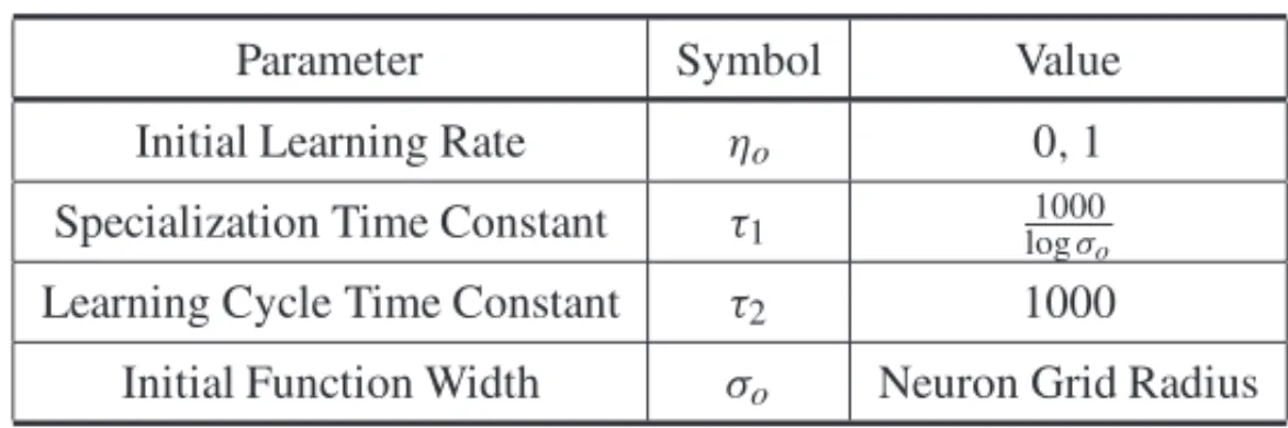
In Figure 2(a) a tendency for a greater phase angle can be observed, with a smaller apparent resistivity. Apparent resistivity is different from real resistivity, only representing the comparison between the object resistivity with reference to the primary medium. Therefore, an object with
resistivity smaller than sea water ρ0is observed. However, it must be noted that the resistive
object is still not visible to the set of sensors, due to the shadowing caused by the conductive object and its distance from the receptors.
Observing the SOM results in Figure 2(a) compared to the original measurements, some neu-rons were fitted off the original data. It can show an algorithmic failure or an actual probability distribution, but it can only been determined with a greater resolution map, with more receptors. However, receptors for this frequency range have great dimensions, which means that only a small number of EM receptors can be placed in the map.
0.17 0.175 0.18 0.185 0.19 0.195 0.2 0.205 0.21 0.215 0.22 0.225 0.23
42.5 43 43.5 44 44.5 45 45.5 46 46.5 47 47.5
ρ
(
Ω
)
ϕ (°)
(a) PhaseφversusApparent Resistivityρ
44.75 45 45.25 45.5 45.75 46 46.25 46.5
-50 -40 -30 -20 -10 0 10 20 30 40 50
ϕ
(°)
x (m)
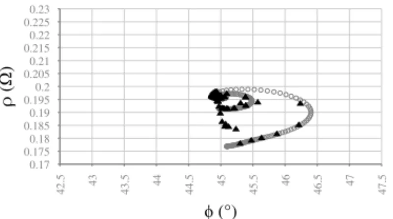
(b) Object Position Along the Sea LineversusPhaseφ
44.75 45 45.25 45.5 45.75 46 46.25 46.5
0 10 20 30 40 50 60 70 80 90
100 110 120 130 140 150 160 170 180 190 200 210 220 230
ϕ
(°)
y (m)
(c) DepthversusPhaseφ
Figure 2: Simulated electromagnetic data (circle) and SOM dimensionality reduction output
(triangle) att =0 s.
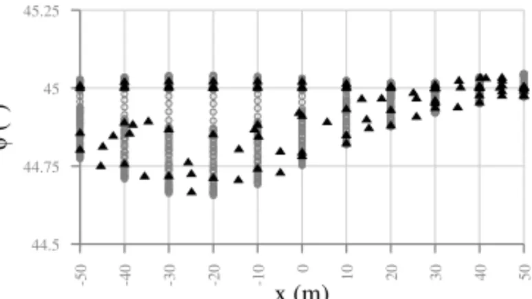
The SOM algorithm results observed in Figure 2(b) fitted this dimension with great accuracy,
with a little or no loss in data. Some neurons are even located in−5 m and 5 m, predicting a high
phase region in this area. So, the SOM maps could, in this case, compensate a resolution loss, placing neurons in regions with lack of receptors.
The Figure 2(c) shows the relationship between phase and the object depth into water. The phase changing position usually represents a change of medium for the electromagnetic wave. In this figure, the conductive object is mapped to be between 10 m and 25 m, within the range of the conductive structure.
Again, the SOM algorithm was able to fit the data in Figure 2(c), even using the probability density estimation inherent to this kind of algorithm to place a “virtual sensor”, as shown in Figure 2(b). The results are consistent with the phase shift of the “virtual sensor” in Figure 2(b), which means that the algorithm isn’t creating spurious data.
Figure 3 presents the next analyzed time step. At 60 s, both objects are observed, as demonstrated in 3(a). This is reassured in the next graphs, where the conductive object appear farther than the
last observation (y=60 m) while the resistive object approaches (y=140 m), making the width
0.194 0.195 0.196 0.197 0.198 0.199 0.2 0.201
44.5 44.6 44.7 44.8 44.9 45 45.1 45.2 45.3 45.4 45.5
ρ
(
Ω
)
ϕ (°)
(a) PhaseφversusApparent Resistivityρ
44.75 45 45.25
-50 -40 -30 -20 -10 0 10 20 30 40 50
ϕ
(°)
x (m)
(b) Object Position Along the Sea LineversusPhaseφ
44.75 45 45.25
0 10 20 30 40 50 60 70 80 90
100 110 120 130 140 150 160 170 180 190 200 210 220 230
ϕ
(°)
y (m)
(c) DepthversusPhaseφ
Figure 3: Simulated electromagnetic data (circle) and SOM dimensionality reduction output
(triangle) att =60 s.
The Kohonen Network Fitted the data with great accuracy, placing again “Virtual Sensors” between the actual ones. These “virtual sensors” didn’t create spurious data, with predictions consistent with the measured data.
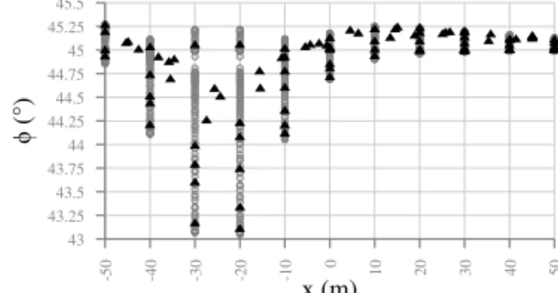
At the time step shown in Figure 4, the resistive object starts do shadow the conductive one, as
shown in 4(a). Now its actual horizontal position can be predicted between−50 m and−10 m,
with side lobes present from 0 m to 30 m. The sea depth of the object is predicted between 80 m and 100 m, range that covers the object. The SOM algorithm fitted well the parameters, again presenting accurate virtual sensors.
In Figure 5, the same behaviour is present, both for the measurement data and SOM algorithm, with accurate virtual sensors. The range of the resistive object can be predicted, with the
barycen-tre predicted by a virtual sensor at−25 m, precisely its position. The object width is reassured,
between−40 m and−10 m. If the SOM virtual sensors is taken into account, the object range
falls to−35 m to−15 m, precisely the object range. The depth of the object can be predicted
between 50 m and 80 m, but the SOM algorithm places the object at 65 m, a 5 m error.
0.194 0.195 0.196 0.197 0.198 0.199 0.2 0.201
44.5 44.6 44.7 44.8 44.9 45 45.1 45.2 45.3 45.4 45.5
ρ
(
Ω
)
ϕ (°)
(a) PhaseφversusApparent Resistivityρ
44.75 45 45.25
-50 -40 -30 -20 -10 0 10 20 30 40 50
ϕ
(°)
x (m)
(b) Object Position Along the Sea LineversusPhaseφ
44.75 45 45.25
0 10 20 30 40 50 60 70 80 90
100 110 120 130 140 150 160 170 180 190 200 210 220 230
ϕ
(°)
y (m)
(c) DepthversusPhaseφ
Figure 4: Simulated electromagnetic data (circle) and SOM dimensionality reduction output
(triangle) att =100 s.
5 CONCLUSION
A dimensionality reduction and feature extraction algorithm for object detection in conductive media using Self-Organizing Maps (SOM) is presented. Using simulated data as input for the SOM algorithm, a set of representative units were fitted to the input data.
The SOM algorithm outputs were able to fit the input data and to attain its probability distribution, generating virtual sensors, neurons fitted in high probability regions, with accurate data, even with a difficult propagation media for the electromagnetic signal such as sea water.
In some cases, the virtual sensors were able to identify the moving objects, helping to differenti-ate them and sometimes precisely predicting their boundaries. The electromagnetic signal alone wasn’t able to get such precise results. Best results were achieved in less extreme situations, in which the objects are further from the sensors and neither of them have a strong predominance in detection.
0.194 0.195 0.196 0.197 0.198 0.199 0.2 0.201
44.5 44.6 44.7 44.8 44.9 45 45.1 45.2 45.3 45.4 45.5
ρ
(
Ω
)
ϕ (°)
(a) PhaseφversusApparent Resistivityρ
44.5 44.75 45 45.25
-50 -40 -30 -20 -10 0 10 20 30 40 50
ϕ
(°)
x (m)
(b) Object Position Along the Sea LineversusPhaseφ
44.5 44.75 45 45.25
0 10 20 30 40 50 60 70 80 90
100 110 120 130 140 150 160 170 180 190 200 210 220 230
ϕ
(°)
y (m)
(c) DepthversusPhaseφ
Figure 5: Simulated electromagnetic data (circle) and SOM dimensionality reduction output
(triangle) att =140 s.
Further work can expand the EM analysis for a three dimensional input and develop a decision making algorithm using artificial intelligence. These algorithms combined can create a decision support software to naval systems. The same feature extraction algorithm can be used in other areas, such as bioelectromagnetics, to detect anomalies in tissues from EM imaging.
RESUMO.O uso do algor´ıtmo de Mapas Auto-Organiz´aveis (SOM) para extrac¸˜ao de ca-racter´ısticas e reduc¸˜ao de dimensionalidade aplicado `a detecc¸˜ao de objetos subaqu´aticos em regi˜oes marinhas foi apresentado. Simulac¸˜oes em Elementos Finitos foram utilizadas para a gerac¸˜ao de um modelo direto da regi˜ao de estudo e, a partir destes dados, um Mapa Auto-Organiz´avel foi utilizado para ajustar os dados e retornar um modelo similar, com dimensio-nalidade menor e mesmas caracter´ısticas. Sensores Virtuais foram criados automaticamente pelo algoritmo SOM com resultados consistentes, completando os vazios de resoluc¸˜ao dos dados simulados. Estes resultados s˜ao ´uteis para acelerar algoritmos de aux´ılio `a tomada de decis˜ao reduzindo o n´umero de entradas destes algoritmos e em outros assuntos, como bioeletromagn´etica.
0.17 0.175 0.18 0.185 0.19 0.195 0.2 0.205 0.21 0.215 0.22 0.225 0.23
42.5 43 43.5 44 44.5 45 45.5 46 46.5 47 47.5
ρ
(
Ω
)
ϕ (°)
(a) PhaseφversusApparent Resistivityρ
43 43.25 43.5 43.75 44 44.25 44.5 44.75 45 45.25 45.5
-50 -40 -30 -20 -10 0 10 20 30 40 50
ϕ
(°)
x (m)
(b) Object Position Along the Sea LineversusPhaseφ
43 43.25 43.5 43.75 44 44.25 44.5 44.75 45 45.25 45.5
0 10 20 30 40 50 60 70 80 90
100 110 120 130 140 150 160 170 180 190 200 210 220 230
ϕ
(°)
y (m)
(c) DepthversusPhaseφ
Figure 6: Simulated electromagnetic data (circle) and SOM dimensionality reduction output
(triangle) att =180 s.
REFERENCES
[1] L.S. Batista. Otimizac¸˜ao computacional da t´ecnica de elementos finitos para o modelamento geof´ısico eletromagn´etico. Master’s thesis, Universidade Federal do Par´a, Par´a (1991).
[2] L.S. Batista & E.E. Sampaio. Scattering of electromagnetic plane waves by a buried vertical dike.
Anais da Academia Brasileira de Ciˆencias,75(2) (2003), 189–207.
[3] S.C. Constable & K.W. Key. Method and system for detecting and mapping hydrocarbon reservoirs using electromagnetic fields, Aug. 28 2012. US Patent 8,253,418.
[4] M.E. Everett. Theoretical developments in electromagnetic induction geophysics with selected appli-cations in the near surface.Surveys in geophysics,33(1) (2012), 29–63.
[5] A.M. Franz, T. Haidegger, W. Birkfellner, K. Cleary, T.M. Peters & L. Maier-Hein. Electromagnetic tracking in medicine – a review of technology, validation, and applications.Medical Imaging, IEEE Transactions on,33(8) (2014), 1702–1725.
[7] Y. Han, F. Wu, D. Tao, J. Shao, Y. Zhuang & J. Jiang. Sparse unsupervised dimensionality re-duction for multiple view data.Circuits and Systems for Video Technology, IEEE Transactions on, 22(10) (2012), 1485–1496.
[8] S. Haykin.Neural Networks: A Comprehensive Foundation. International edition. Prentice Hall International (1999).
[9] E.C. Jordan & K.G. Balmain.Electromagnetic waves and radiating systems, volume 4. Prentice-Hall Englewood Cliffs, NJ (1968).
[10] K. Key. Marine electromagnetic studies of seafloor resources and tectonics.Surveys in geophysics, 33(1) (2012), 135–167.
[11] T. Kohonen. The self-organizing map.Neurocomputing,21(1) (1998), 1–6.
[12] W. Li, S. Prasad, J.E. Fowler & L.M. Bruce. Locality-preserving dimensionality reduction and clas-sification for hyperspectral image analysis.Geoscience and Remote Sensing, IEEE Transactions on, 50(4) (2012), 1185–1198.