Family Dependence in 331 Models
R. Mart´ınez and F. Ochoa
Universidad Nacional de Colombia, Ciudad Universitaria, Carrera 30, No. 45-03, Edificio 405 Oficina 218, Bogota, Colombia
Received on 16 October, 2006
Using experimental results at the Z-pole, and considering the ansatz of Matsuda as an specific texture for the quark mass matrices, we perform aχ2 fit at 95% CL to obtain family-dependent bounds toZ′mass and Z-Z’ mixing angle in the framework of the main versions of 331 models. The allowed regions depend on the assignment of the physical quark families into different representations that cancel anomalies. Allowed regions on other possible 331 models are also obtained.
Keywords: Standart model; Gauge bosons
I. INTRODUCTION
In most of extensions of the standard model (SM), new massive and neutral gauge bosons, called Z′, are predicted. The presence of this boson is sensitive to experimental obser-vations at low and high energies, and will be of great interest in the next generation of colliders (LHC, ILC, TESLA) [1]. In particular, it is possible to study some phenomenological features associated toZ′ through models with gauge symme-trySU(3)c⊗SU(3)L⊗U(1)X,also called 331 models. These models arise as an interesting alternative to explain the origin of generations [2–4], where the three families are required in order to cancel chiral anomalies. The electric charge is de-fined as a linear combination of the diagonal generators of the group
Q=T3+βT8+X I, (1) whereβallow classify the different 331 models. The two main versions corresponds toβ=−√3 [2] andβ=−√1
3[3]. In the quark sector, each 331-family can be assigned in 3 different ways. Therefore, in a phenomenological analysis, the allowed region associated with theZ−Z′mixing angle and the physi-cal massMZ′ ofZ′will depend on the family assignment. We adopt the texture structure proposed in ref. [5] in order to ob-tain allowed regions for theZ−Z′mixing angle, the mass of theZ′boson and the values ofβfor 3 different assignments of the quark families in mass eigenstates. The above analysis is performed through aχ2statistics at 95% CL.
II. THE QUARK AND NEUTRAL GAUGE SPECTRUM
The fermion representations under SU(3)c⊗ SU(3)L⊗ U(1)Xread
b ψL =
½ b
qL: ¡
3,3,XqL¢=¡3,2,XqL¢⊕¡3,1,XqL¢,
b
ℓL:¡1,3,XℓL¢=¡1,2,XℓL¢⊕¡1,1,XℓL¢, b
ψ∗L =
½ b
q∗ L:
¡
3,3∗,−XqL¢=¡3,2∗,−XqL¢⊕¡3,1,−XqL¢,
b
ℓ∗ L:
¡
1,3∗,−XℓL¢=¡1,2∗,−XℓL¢⊕¡1,1,−XℓL¢,
b ψR =
½ b
qR: ¡
3,1,XqR¢,
b
ℓR:¡1,1,XℓR¢.
(2)
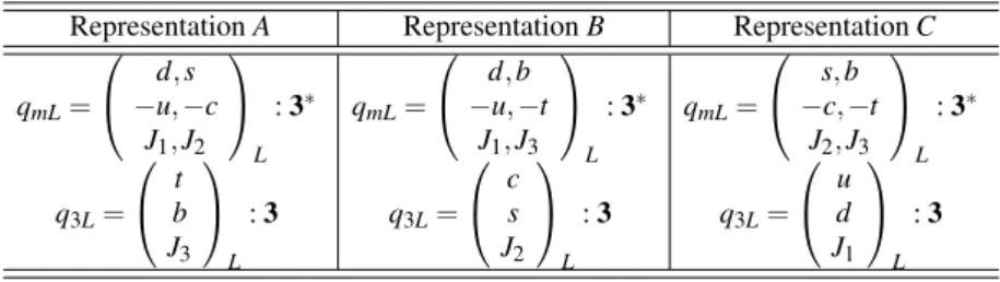
The second equality comes from the branching rules SU(2)L⊂SU(3)L. TheXprefers to the quantum number as-sociated withU(1)X. The generator ofU(1)X conmute with the matrices ofSU(3)L; hence, it should take the formXpI3×3, the value ofXpis related with the representations ofSU(3)L and the anomalies cancellation. On the other hand, this fermi-onic content shows that the left-handed multiplets lie in either the3 or3∗representations. In the framework of three fam-ily model, we recognize 3 different possibilities to assign the physical quarks in each family representation as shown in Ta-ble I in weak eigenstates.
On the other hand, we obtain the following mass eigenstates associated to the neutral gauge spectrum
Z1µ = ZµCθ+Z′µSθ; Z2µ=−ZµSθ+Zµ′Cθ, (3) where a small mixing angleθbetween the neutral currentsZµ andZµ′ appears, with
Zµ = CWWµ3−SW µ
βTWWµ8+ q
1−β2T2 WBµ
¶ ;
Z′µ = −
q
1−β2T2 WW
8
µ+βTWBµ, (4) where the Weinberg angle is defined as SW = g′/(pg2+ (1+β2)g′2)andg,g′ correspond to the coupling constants of the groupsSU(3)LandU(1)X,respectively.
III. THE NEUTRAL GAUGE COUPLINGS
The neutral Lagrangian associated to the SM-bosonZ1µin the weak basis of the SM quarksU0=¡u0,c0,t0¢T andD0= ¡
d0,s0,b0¢T,is
L
NC = g2CW n
U0γ µ
h
GUv(r)−GUa(r)γ5 i
U0 +D0γ
µ h
GDv(r)−GDa(r)γ5 i
RepresentationA RepresentationB RepresentationC
qmL=
d,s −u,−c
J1,J2
L
:3∗
q3L=
t b J3 L :3
qmL=
d,b −u,−t
J1,J3
L
:3∗
q3L=
c s J2 L :3
qmL=
s,b −c,−t
J2,J3
L
:3∗
q3L=
u d J1 L :3
TABLE I: Three different family structures in the fermionic spectrum
δgV(r,)A=ge(Vr,)ASθ, (6) which corresponds to the correction due to the smallZµ− Zµ′ mixing angle θ, geV(r,)Athe Zµ′ coupling constants, and r= (A,B,C)each representation from Table I. TheZ′
µcouplings for leptons are
∼
gℓv,a= g′CW 2gTW
·
−1 √
3−βT 2
W±2QℓβTW2 ¸
, (7)
while for the quark couplings we get
∼
gqv,(ar)= g′CW 2gTW
K(r)†¡M±2QqβTW2¢K(r), (8)
with q = U0,D0, M = 1/√3diag[1 + βTW2/√3,1 + βTW2/√3,−1+βTW2/√3] and where we define for each representation from table I
K(A)=I,K(B)=
1 0 00 0 1
0 1 0
, K(C)=
0 1 00 0 1
1 0 0
. (9)
We will consider linear combinations among the three fam-ilies to obtain couplings in mass eigenstates by adopting an ansatz on the texture of the quark mass matrix in agree-ment with the CKM matrix. We take the structure of mass matrix suggested in ref. [5] given by Mq′ =Pq†MPq†, with Pq=diag(exp(α1),exp(α2),exp(α3)), and whereM is writ-ten in the basis¡u0,c0,t0¢or¡d0,s0,b0¢as
Mq=
0
Aq Aq Aq Bq Cq Aq Cq Bq
. (10)
For up-type quarks,AU= pmtmu
2 ,BU= (mt+mc−mu)/2 and CU = (mt−mc−mu)/2; for down-type quarks AD = q
mdms
2 , BD = (mb+ms−md)/2 and CD =−(mb−ms+
md)/2. The above ansatz is diagonalized by [5]
RD=
c s 0
−√s
2 c √ 2 − 1 √ 2
−√s
2 c √ 2 1 √ 2
; RU =
c′ 0 s′ −√s′
2 − 1 √ 2 c′ √ 2
−√s′
2 1 √ 2 c′ √ 2 , (11) with c = pms/(md+ms),s =
p
md/(md+ms),c′ = p
mt/(mt+mu) and s′ = p
mu/(mt+mu). The complex matrix M′
q=Pq†MPq† is then diagonalized by the bi-unitary transformationULq†Mq′URq withULq=Pq†RqandURq=PqRq. Then, the diagonal couplings in Eq. (5) in mass eigenstates have terms of the formUL†,RqGvq,(ar)UL,Rq =R†qG
q(r)
v,a Rq where any effect of the CP violating phasesPdisappears. Thus, we can write the Eq. (5) in mass eigenstates as
L
NC = g2CW h
Uγµ ³
GUv(r)−GUa(r)γ5 ´
U +Dγµ
³
GDv(r)−GDa(r)γ5 ´
DiZ1µ, (12)
where the couplings of quarks depend on the rotation ma-trix, with
Gqv,(ar)=gqv,aI+R†qδg q(r)
v,a Rq=gqv,aI+δg q(r)
v,a . (13)
δZ = ΓSM
u ΓSM
Z
(δu+δc) + ΓSM
d ΓSM
Z
(δd+δs)
+Γ SM b ΓSM
Z δb+3
ΓSM ν ΓSM
Z δν+3
ΓSM e ΓSM
Z δℓ;
δhad = RSMc (δu+δc) +RSMb δb+ ΓSM
d ΓSM
had
(δd+δs);
δσ = δhad+δℓ−2δZ;
δAf = δgVf f
gVf + δgAf f
gAf − δf,
δQW = ∆QW
QWSM (14)
where
δf =
2gvfδgvf f+2gaδgf af f ³
gvf ´2
+³gaf
´2 ,
∆QW ≃ −0.01+∆Q′W, (15)
∆QW ≃ −0.01−16(2Z+N) h³
geA∼guuv +∼geaguV´ + (Z+2N)
µ
gea∼gddv +∼geagdv
¶¸
Sθ
−16 ·
(2Z+N)∼gea∼gvuu+ (Z+2N)∼gea∼gddv ¸M2
Z1
MZ2
2
.
(16)
-
0.2
-
0.1
0
0.1
0.2
0.3
Sin
Θ
H10
-3L
0
10
20
30
40
50
60
M
Z2
H
10
3
GeV
L
A
-
B
Β = -
!!!
3
C
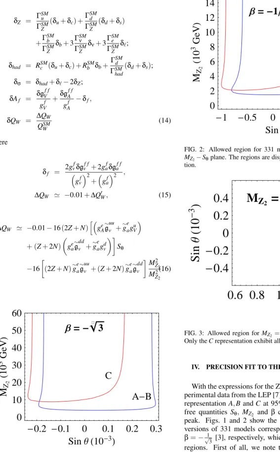
FIG. 1: Allowed region for 331 models withβ=−√3 in theMZ2− Sθplane. The regions are dispayed forA,BandCrepresentation.
-
1
-
0.5
0
0.5
1
1.5
Sin
Θ
H10
-3L
0
2
4
6
8
10
12
14
M
Z2
H
10
3
GeV
L
Β = -
1
!!!
3
A
-
B
C
FIG. 2: Allowed region for 331 models withβ=−1/√3 in the MZ2−Sθplane. The regions are dispayed forA,BandC
representa-tion.
0.6 0.8
1
1.2 1.4 1.6
Β
-0.4
-0.2
0
0.2
0.4
Sin
Θ
H
10
-3
L
C
M
Z2
=
1200 GeV
FIG. 3: Allowed region forMZ2=1200 GeV in theSθ−βplane.
Only theCrepresentation exhibit allowed region.
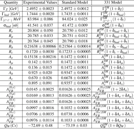
IV. PRECISION FIT TO THE Z-POLE OBSERVABLES
With the expressions for the Z-pole observables and the ex-perimental data from the LEP [7], we perform aχ2fit for each representationA,BandC at 95% CL and 3 d.o.f, where the free quantities Sθ, MZ2 andβ can be constrained at the Z1
peak. Figs. 1 and 2 show the allowed region for the main versions of 331 models corresponding toβ=−√3 [2] and β=−√1
3 [3], respectively, which exhibits family-dependent regions. First of all, we note that A and B representations display broader mixing angles than representationC. For the model β=−√3, we see that the lowest bound in the MZ2
Quantity Experimental Values Standard Model 331 Model ΓZ[GeV] 2.4952±0.0023 2.4972±0.0012 ΓSMZ (1+δZ)
Γhad[GeV] 1.7444±0.0020 1.7435±0.0011 ΓSMhad(1+δhad)
Γ(ℓ+ℓ−)MeV 83.984±0.086 84.024±0.025 ΓSM(ℓ+ℓ−)(1+δℓ) σhad[nb] 41.541±0.037 41.472±0.009 σSMhad(1+δσ)
Re 20.804±0.050 20.750±0.012 RSMe (1+δhad+δe)
Rµ 20.785±0.033 20.751±0.012 RSMµ
¡
1+δhad+δµ¢
Rτ 20.764±0.045 20.790±0.018 RSMτ (1+δhad+δτ)
Rb 0.21638±0.00066 0.21564±0.00014 RbSM(1+δb−δhad)
Rc 0.1720±0.0030 0.17233±0.00005 RSMc (1+δc−δhad)
Ae 0.15138±0.00216 0.1472±0.0011 ASMe (1+δAe)
Aµ 0.142±0.015 0.1472±0.0011 ASMµ
¡
1+δAµ¢
Aτ 0.136±0.015 0.1472±0.0011 ASMτ (1+δAτ)
Ab 0.925±0.020 0.9347±0.0001 ASMb (1+δAb)
Ac 0.670±0.026 0.6678±0.0005 ASMc (1+δAc)
As 0.895±0.091 0.9357±0.0001 ASMs (1+δAs)
AFB(0,e) 0.0145±0.0025 0.01626±0.00025 AFB(0,e)SM(1+2δAe)
AFB(0,µ) 0.0169±0.0013 0.01626±0.00025 AFB(0,µ)SM¡1+δAe+δAµ
¢
AFB(0,τ) 0.0188±0.0017 0.01626±0.00025 AFB(0,τ)SM(1+δAe+δAτ)
AFB(0,b) 0.0997±0.0016 0.1032±0.0008 AFB(0,b)SM(1+δAe+δAb)
AFB(0,c) 0.0706±0.0035 0.0738±0.0006 AFB(0,c)SM(1+δAe+δAc)
AFB(0,s) 0.0976±0.0114 0.1033±0.0008 AFB(0,s)SM(1+δAe+δAs)
QW(Cs) −72.69±0.48 −73.19±0.03 QWSM(1+δQW)
TABLE II: The Z-pole parameters for experimental values, SM predictions and 331 corrections.
-
1.5
-
1
-
0.5 0 0.5 1 1.5
Β
1
2
3
4
5
6
7
8
M
Z2
H
10
3
GeV
L
A
-
B
Sin
Θ = -
0.0002
C
FIG. 4: Allowed region forSθ=−0.0002 in theMZ2−βplane. The regions are dispayed forA,BandCrepresentations.
β=−√1
3 exhibits a lower bound in the Z2 mass, where the lowest bound is about 1400 GeV for A andB regions, and 2100 GeV for theCspectrum. We also see that the mixing an-gle in this model is smaller by about one order of magnitude than the angles predicted by theβ=−√3 model.
On the other hand, we get the best allowed region in the planeSθ−βfor two different values ofMZ2. The lowest bound
that display an allowed region is about 1200 GeV, which
ap-pears only for theC assignments such as Fig. 3 shows. We can see in this case that the usual 331 models are excluded, and only those 331 models with 1.1.β.1.75 are allowed with small mixing angles (Sθ∼10−4). Fig. 4 display the al-lowed region in theMZ2−βplane for a small mixing angle
(Sθ=−0.0002).It is noted that the smallest bounds inMZ2is
[1] S. Godfrey arXiv: hep-ph/0201093; G. Weiglein et. al., arXiv: hep-ph/0410364; R.D. Heuer et. al, arXiv: hep-ph/0106315. [2] F. Pisano and V. Pleitez, Phys. Rev. D 46, 410 (1992); P.H.
Frampton, Phys. Rev. Lett.69, 2889 (1992).
[3] R. Foot, H.N. Long, and T.A. Tran, Phys. Rev. D50, R34 (1994). [4] L.A. S´anchez, W.A. Ponce, and R. Mart´ınez, Phys. Rev. D64, 075013 (2001);Rodolfo A. Diaz, R. Martinez, and F. Ochoa, Phys. Rev. D69, 095009 (2004); Rodolfo A. Diaz, R. Martinez,
and F. Ochoa, Phys. Rev. D72,035018 (2005).