ISSN: 1809-4430 (on-line)
_________________________
1 Parte da Tese de Doutorado desenvolvida pelo primeiro autor. Projeto financiado pela FAPEMIG, CAPES e CNPq
2 Engº Civil, Prof. Doutor, Coordenadoria de Saneamento Ambiental, IFES/Colatina-ES, Fone: (27) 3723-1509: [email protected] 3 Engº Agrônomo, Prof. Doutor, Departamento de Engenharia Agrícola, UFV/Viçosa – MG, [email protected]
4 Engº Agrônomo, Prof. Doutor, Departamento de Engenharia Agrícola, UFV/Viçosa – MG, [email protected] 5 Eng. Civil, Prof. Doutor, Curso de Engenharia Civil, UFPel/Pelotas-RS, [email protected]
6 Engº Agrônomo, Prof. Doutor, Departamento de Engenharia Florestal, UFV/Viçosa – MG, [email protected] 7Engº Civil, Prof. Doutor, Departamento de Engenharia Sanitária e Ambiental, UFJF/Juiz de Fora –
MULTIVARIATE STATISTICAL ANALYSIS TO SUPPORT THE MINIMUM STREAMFLOW REGIONALIZATION
Doi:http://dx.doi.org/10.1590/1809-4430-Eng.Agric.v35n5p838-851/2015
ABRAHÃO A. A. ELESBON2, DEMETRIUS D. DA SILVA3, GILBERTO C. SEDIYAMA4,
HUGO A. S GUEDES5, CARLOS A. A. S. RIBEIRO6, CELSO B. DE M. RIBEIRO7
ABSTRACT: This study aimed to develop a methodology based on multivariate statistical analysis of principal components and cluster analysis, in order to identify the most representative variables in studies of minimum streamflow regionalization, and to optimize the identification of the hydrologically homogeneous regions for the Doce river basin. Ten variables were used, referring to the river basin climatic and morphometric characteristics. These variables were individualized for each of the 61 gauging stations. Three dependent variables that are indicative of minimum streamflow (Q7,10, Q90 and Q95). And seven independent variables that concern to climatic and
morphometric characteristics of the basin (total annual rainfall – Pa; total semiannual rainfall of the
dry and of the rainy season – Pss and Psc; watershed drainage area – Ad; length of the main river –
Lp; total length of the rivers – Lt; and average watershed slope – SL). The results of the principal
component analysis pointed out that the variable SL was the least representative for the study, and
so it was discarded. The most representative independent variables were Ad and Psc. The best
divisions of hydrologically homogeneous regions for the three studied flow characteristics were obtained using the Mahalanobis similarity matrix and the complete linkage clustering method. The cluster analysis enabled the identification of four hydrologically homogeneous regions in the Doce river basin.
KEYWORDS:principal component analysis, cluster analysis, homogeneous regions.
ESTATÍSTICAS MULTIVARIADAS COMO SUPORTE À REGIONALIZAÇÃO DE VAZÕES MÍNIMAS1
RESUMO: Este trabalho teve por objetivo propor uma metodologia baseada em análises estatísticas multivariadas de componentes principais e de agrupamento, com o intuito de identificar as variáveis mais representativas em estudos de regionalização de vazões mínimas e otimizar a obtenção das regiões hidrologicamente homogêneas para a bacia hidrográfica do Rio Doce. Foram utilizadas 10 variáveis referentes às características climáticas e morfométricas da bacia. Essas variáveis foram individualizadas para as 61 estações fluviométricas adotadas, sendo três variáveis dependentes e indicativas das vazões mínimas (Q7,10, Q90 e Q95) e sete independentes (precipitação
total anual – Pa; precipitação total do semestre seco –Pss e chuvoso –Psc; área de drenagem da bacia –
Ad; comprimento do rio principal – Lp; comprimento total dos cursos d’água da bacia – Lt; e
declividade média da bacia – SL). O resultado da análise de componentes principais apontou a
variável independente SL como a menos representativa e foi excluída do estudo. As variáveis
independentes mais representativas foram Ad e Psc. As melhores divisões de regiões
hidrologicamente homogêneas para as três vazões características estudadas foram obtidas utilizando-se conjuntamente da matriz de similaridade de Mahalanobis e do método de agrupamento do vizinho mais distante. A análise de agrupamento possibilitou a identificação de quatro regiões hidrologicamente homogêneas na bacia hidrográfica do Rio Doce.
INTRODUCTION
The hydrological performance of a river basin depends on its geomorphological characteristics, climate aspects and the type of plant coverage. Thereby, several physical and biotic variables of a basin play an important role in the hydrological cycle processes.
River basins with large drainage areas can present different hydrological performances in distinct parts. For that reason, the identification of hydrological homogeneity of a determined region is one of the first goals to be reached in order to have a correct water resources management.
Hydrological generalization is defined as any process of transferring information from one region of identified hydrological performance to other places, usually without observations. This transfer can be directly reported to data series, or to certain relevant statistical parameters such as average, variance, maximum and minimum events, or even equations and parameters related to these statistical parameters.
MISHRA & COULIBALY (2009) describe the importance of having reliable information in a watershed scope due to its innumerous practical uses: hydrology, agronomy, climatology, hydrogeology, management and planning of water resources, decision processes for implementation of public policies and industrial plants installations.
In this context, multivariate statistical analyses can expressively assist the conduction of hydrological generalization studies, reducing the processing time of database and increasing the reliability of obtained results. In an international level, this affirmation can be ascertained through the development of several studies aiming hydrological generalization (ASSANI et al., 2011; MWALE et al., 2011; SAMUEL et al., 2011; ENGELAND & HISDAL, 2009; CASTIGLIONI et al., 2009).
The principal component analysis aims to review the correlations between studied variables, to summarize a large set of variables in a smaller one and in an equivalent purpose, to evaluate the importance of each variable and to promote the elimination of the ones that contribute little, in terms of variation, in the group of evaluated individuals (WILKS, 2006).
Over the past years, this technique has been used in a variety of domains, including medicine (SILVA et al., 2010), remote sensing (JESUS & EPIPHANIO, 2010), farming (ARRUDA et al., 2012; ARRUDA et al., 2011; YAMAKI et al., 2009), chemistry (BELLOMARINO et al., 2010; FARO JR. et al., 2010), analysis of soil (ISLABÃO et al., 2013), environmental studies (GUEDES et al., 2012; REID & SPENCER, 2009) among others.
Clustering multivariate statistical analysis is a data exploratory tool that aims to classify homogeneous groups (WILKS, 2006). It has been employed in several areas of knowledge, for instance, genetics (CARVALHO et al., 2009), management (COUTO JR & GALDI, 2012), health (RESENDES et al., 2010) and environmental engineering (HATVANI et al., 2011). In hydrology, cluster analysis is a technique often used to define classes or to group stations into homogeneous climate regions, i.e. regionalization.
In light of the above, this study aimed at developing a methodology based on multivariate statistical analyses of principal component and cluster analysis, targeting the identification of the most representative variable in studies of minimum streamflow regionalization, as well as to optimize the obtainment of hydrological homogeneous regions for the Doce river basin.
MATERIAL AND METHODS Region of study
Brazilian biome called Atlantic Rainforest and the rest belongs to the Cerrado biome. The leading developed economic activities are mining, metallurgy, forestry and farming (CBH-Doce, 2010).
Database and Applications
The study was conducted using data from 61 gauging stations belonging to hydro meteorological network of the National Water Agency – NWA. The employed series consisted of daily data of flow corresponding to the base period from 1976 to 2005 (Table 1). It is highlighted that the use of data up to the year 2005 was limited due to the fact that, in the beginning of the study, this was the most recent year with consisted data provided by NWA.
The vector base of elevation (contour lines and elevated points) and of hydrography of the hydrographic region obtained with the Brazilian Institute of Geography and Statistics– IBGE at a scale of 1:250.000.
The generation of hydrographically conditioned digital elevation methods (HCDEM), the automatic achievement of morphometric variables, of average precipitations and the spatialization of results were conducted with the aid of the ArcGIS® 10.0 software, as a geoprocessing tool of vectors and spatial representation of data.
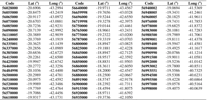
TABLE 1. Gauging stations selected for a minimum streamflow regionalization.
Code Lat (o) Long (o) Code Lat (o) Long (o) Code Lat (o) Long (o)
56028000 -20.6906 -43.2994 56640000 -19.9711 -43.4567 56940002 -19.0694 -41.5369
56055000 -20.8475 -43.2419 56659998 -19.7656 -43.0328 56948005 -19.3431 -41.2461
56065000 -20.9117 -43.0972 56696000 -19.5244 -42.6550 56960005 -20.1825 -41.9611
56075000 -20.6703 -43.0881 56719998 -19.3278 -42.3975 56976000 -19.7431 -41.7853
56085000 -20.7236 -42.9231 56750000 -19.0144 -43.4461 56978000 -19.6825 -41.8372
56090000 -20.7139 -42.9992 56765000 -18.9661 -43.2431 56983000 -20.1081 -41.7283
56110005 -20.3889 -42.9039 56775000 -19.2322 -43.0200 56988500 -19.7989 -41.7061
56240000 -20.3769 -43.1919 56787000 -19.3319 -43.0703 56989001 -19.8111 -41.4378
56335001 -20.3625 -43.1439 56800000 -18.8947 -43.0825 56989400 -19.5947 -41.4581
56337000 -20.2856 -43.0989 56825000 -19.1881 -42.4228 56990000 -19.4925 -41.1617
56385000 -20.6836 -42.6725 56845000 -18.8947 -42.7125 56990990 -20.0786 -41.1214
56415000 -20.2261 -42.6500 56846000 -18.9517 -42.3592 56991500 -19.9011 -41.0581
56425000 -19.9947 -42.6742 56850000 -18.8831 -41.9503 56992000 -19.5236 -41.0142
56460000 -20.2772 -42.3256 56860000 -18.3611 -42.6050 56993002 -19.7800 -40.8511
56484998 -20.1036 -42.4400 56870000 -18.2000 -42.4547 56993551 -19.5586 -40.7325
56500000 -20.2989 -42.4781 56880000 -18.2500 -42.0667 56994500 -19.5308 -40.6231
56510000 -20.0975 -42.4592 56891900 -18.5747 -42.9178 56995500 -19.4228 -40.6864
56520000 -19.9989 -42.3486 56900000 -18.2392 -41.7311 56997000 -19.0578 -40.5164
56539000 -19.7769 -42.4764 56915500 -18.4594 -41.8075 56998000 -19.4075 -40.0639
56570000 -19.7086 -42.4456 56920000 -18.9711 -41.6392
56610000 -19.9317 -43.1731 56935000 -19.3736 -42.1050
The multivariate statistical analyses were conducted with the Statistica® 7.0 software and the multiple regression equations were obtained with the aid of SisCORV 1.0.3 software (SOUSA et al. 2008) developed by the Research Group of Water Resources, linked to the Department of Agricultural Engineering of the Viçosa Federal University.
In the present study, 10 variables were considered, as three were dependent variables to be regionalized (minimum average flow of seven consecutive days and recurrence period of ten years - Q7,10; and the minimum streamflow associated with permanence in time of 90% - Q90 and 95% - Q95)
and seven independent variables (total annual rainfall – Pa, total semiannual rainfall of the dry
season–Pss and rainy season – Psc,in mm; watershed drainage area – Ad,in km²; length of the main
river –Lp,in km; total length of the rivers –Lt,in km; and average watershed slope –SL,in %). Principal component analysis
Based on the principal components analysis, the original set of observed independent variables (Pa, Pss, Psc, Ad, Lp, Lt and SL) was transformed into a new set of variables, named
a) Considering that Yi is a principal component of data matrix, it will be a linear
combination among the seven independent variables regarded; b) The sum of the coefficients square aij is equal to 1; c) each principal component has its own coefficients;
d) the components are not correlated, which means that they are independent of one another;
e) among all the components, Y1 presents the greatest variance, Y2 the second greatest and so forth;
f) the sum of variances of each principal component (Yi) is equal to the sum of variances of each variable (Xj).
As R is a symmetric correlation matrix, of dimensions p x p, from which the eigenvalues (λi) and the eigenvectors (ai) are extracted, the solution was achieved by solving the system (eq. 1):
(1) In which,
λi – are the root characteristics (or eigenvalues) of R matrix. There are p eigenvalues
corresponding to the variances of each one of the p principal components;
I– is the identity matrix of p x p dimension;
ai – eigenvector or characteristic vector or a p x 1 matrix, containing the p coefficients for
each eigenvalue λi corresponding to Yi principal component, Φ – is a zero vector, of p x 1 dimension.
One of the most common problems found in the application of multivariate statistical models is that these depend on the unities and scales in which the variables were measured. The data of variables were standardized through the [eq. (2)], eliminating the dependence of unities and scales in which the variables were presented:
(2) in which,
Zij–standardized variable;
σ(Xj)– standard deviation, and – average of j-th original variable.
The importance of each principal component was evaluated through the existing correlation with each Xj variable, which is (eq. 3):
(3) The following criteria were used to select the principal components in this study:
accumulated percentage of original data total variance greater or equal to 75% (JOLLIFE, 2002); and
Cluster analysis
The cluster process was based on two steps: firstly, the estimation of Mahalanobis similarity between the 61 grouped gauging stations and secondly the adoption of a cluster technique between the single linkage method and complete linkage method, to form the groups.
When Euclidean distance is used for cluster analysis, all variables must be considered not correlated among themselves, although this presumption is usually ignored. In order to avoid this common problem in studies of hydrological generalization, a matrix of similarities was constituted with Mahalanobis distance. In practice, Mahalanobis distance is summarized in the application of the Euclidean distance (eq. 4) to the standardized matrix of data.
(4) In which,
Zij and Zzj – observations of i-th and z-th gauging stations (i = 1, 2, …, n andz = 1, 2, …, n),
with reference to j-th variable or absolute frequency in each studied class (j = 1, 2, …, p).
The single linkage method consists, initially, of a distance matrix (dissimilarity) between gauging stations (individuals). The two most similar individuals were identified (by smaller distance between them) and were reunited in the initial group. In sequence, the distance from the first group in relation to the other individuals was calculated.
The distance between a group and an individual was provided through the expression (eq. 5):
(5) Which means, the distance between the group constituted of the individuals a and b and the individual c was provided by the smallest element from the set of distances of the pairs ac and bc.
From the identification of the smallest distances between the constituted group and the neighboring individuals, a new matrix of dissimilarity was developed of smaller dimensions compared to the initial group and the most similar individuals and/or groups were identified. They were then either incorporated into the initial group or arranged into a second group, depending on whether or not the smallest distance of the new matrix of dissimilarity had been visualized between two other individuals.
In the subsequent stages, increasingly smaller dissimilarity matrices were employed, completing the grouping of all individuals in a single group and composing a dendrogram or tree.
The complete linkage clustering method presents a procedure similar to single linkage method, with one important difference: in each stage, the distance was given by the one that enabled the greatest distance between two individuals and/or groups.
The distance between a group and an individual was provided by the expression: (eq. 6):
(6) which means, the distance between the group constituted by the individuals a and b and the individual c was provided by the greatest element of the distance between sets of pairs of ac and bc.
The definition of the number of homogeneous regions of flow characteristics was carried out using the criterion of inertia between jumps, in which the first visible discontinuity of the graphic is defined as ‘cut-off’ (MELO JÚNIOR et al., 2006; RENCHER, 2002; WILKS, 2006).
Multiple regression analysis
The regression models used to create regionalization equations for each hydrologically homogeneous region were linear, potential, exponential, logarithmic and reciprocal.
The models resulting from the application of multiple regression considered in the hydrologically homogeneous regions provided by the cluster analysis, were selected through the following observations:
representative equation of the studied event;
lower number of independent variables according to the relative significance provided by the principal components analysis;
greater values of adjusted determination coefficient; lower values of factorial standard-error;
significant results by the F test; continuity of flows; and
Convenience of geographic spatialization of the obtained equations.
In order to verify the adjustment of the adopted regression models to the data, an adjusted determination coefficient (r²a 0.70), a standard error of estimate lower than 0.5 (EP < 0.5) and a significance level of 5% by F test, were used.
RESULTS AND DISCUSSION Principal components analysis
Based on the seven independent variables used (Pa, Pss, Psc, Ad, Lp, Lt e SL) for each one of the
61 gauging stations adopted, analysis of the principal components was conducted. The total variance existing in the set of analyzed multivariate data was equal to the number of analyzed variables after data samples were standardized with average and variance equal to 0 and 1, respectively.
In Table 2, the correlation matrix between the standardized independent variables is displayed. In order to evaluate the importance of each variable and promote the elimination of the ones that contribute little in terms of variation, the principal components for the studied variables were identified in the group of individuals evaluated in the regionalization analysis of flows (Table 3).
TABLE 2. Correlation matrix R between the independent variables considered.
Variables Pa Pss Psc Ad Lp Lt SL
Pa 1.00 0.65 0.99 -0.04 -0.02 -0.04 -0.06
Pss 1.00 0.57 -0.08 -0.07 -0.08 -0.18
Psc 1.00 -0.02 0.01 -0.02 -0.06
Ad 1.00 0.94 1.00 -0.10
Lp 1.00 0.94 -0.11
Lt 1.00 -0.10
SL 1.00
Caption: Pa– average total annual rainfall; Pss– average total semiannual rainfall of the dry season; Psc– average total semiannual
rainfall of the rainy season; Ad - watershed drainage area; Lp - length of the main river; Lt - total length of the rivers and SL - average
Table 3. Principal components (CP) of studied variables.
CP eigenvalue Variance % Var. % acum. Z Coefficients of standardized variables
1 (Pa) Z2 (Pss) Z3 (Psc) Z4 (Ad) Z5 (Lp) Z6 (Lt) Z7 (SL)
Y1 2.9628 42.33% 42.33% 0.1216 0.1310 0.1035 -0.5679 -0.5544 -0.5679 0.0700
Y2 2.4911 35.59% 77.92% 0.6025 0.4858 0.5889 0.1074 0.1207 0.1072 -0.1286
Y3 0.9950 14.21% 92.13% 0.1430 -0.1534 0.1628 0.0519 0.0427 0.0497 0.9605
Y4 0.4733 6.76% 98.89% 0.2541 -0.8447 0.4032 -0.0463 -0.0139 -0.0362 -0.2361
Y5 0.0755 1.08% 99.97% 0.0222 -0.0123 0.0068 0.3960 -0.8220 0.4082 -0.0124
Y6 0.0020 0.03% 99.996% -0.7317 0.0976 0.6726 0.0369 -0.0144 -0.0330 0.0108
Y7 0.0003 0.004% 100.000% 0.0379 -0.0108 -0.0307 0.7092 -0.0066 -0.7032 -0.0039
According to HELENA et al. (2000), correlation coefficients superior to 0.5 express a strong relationship between evaluated variables. Table 2 demonstrates that climate variables Pa and Psc are
strongly correlated to one another and variable Pss is moderately correlated to variables Pa and Psc.
Morphometric variables Ad, Lp and Lt are highly correlated to one another, however the
morphometric variable SL presents weak correlation to the remaining analyzed variables (R<0.5),
which indicates that it should possibly be excluded from this study.
Based on data presented on Table 3, only the two first components (Y1 and Y2) were
considered, as they simultaneously met two adopted criteria of selection (the accumulated variance explaining a value greater or equal to 75% of the total data variation and eigenvalues greater or equal to 1). The other components were not considered, which together explained 22.08% of the total variation. Table 4 presents the correlations, or load factors, between the seven standardized variables and the two first principal components.
TABLE 4. Load factors between the standardized variables (VP) and the principal components (CP) and variance (λi) of each principal component (i = 1, 2).
X VP Y CP
1 Y2
Pa Z1 0.209226 0.950899
Pss Z2 0.225520 0.766821
Psc Z3 0.178086 0.929543
Ad Z4 -0.977547 0.169484
Lp Z5 -0.954338 0.190567
Lt Z6 -0.977535 0.169216
SL Z7 0.120541 -0.202970
(%) λi 42.33 35.59
It is observed on Table 4 that the standardized variables Z4, Z5 and Z6 present greater
correlations with the first principal component (Y1), while the variables Z1, Z2 and Z3 indicate
greater correlations with the second principal component (Y2). The variable Z7 can be discarded
from the study as it contributes little to the group of evaluated individuals in terms of variation, confirming the result obtained by the analysis of correlation matrix R.
The average watershed slope (SL) variable presents insignificant representativeness in relation
to the performance of studied flow characteristics, as it defines a uniform surface of all drainage areas, which does not physically represent the natural process of river channel runoff. For this reason, the exclusion of the variable SL from the selected set was expected.
The monitoring of water resources involves a great number of variables and the quantitative reduction of unnecessary information directly leads to savings in time and resources. MISHRA & COULIBALY (2009) demonstrated in their study, the importance of having reliable variables in engineering studies in a watershed. CASTIGLIONI et al. (2009) also used physiographic variables when trying to identify hydrologically homogeneous regions.
Physically, the principal component Y1 represents the most representative morphometric
variables and the principal component Y2 represents the average rainfalls in drainage areas upwind
According to WILKS (2006), the obtained results showed that the use of principal components tool for the regionalization of flows, even in a preliminary way, is fundamental to the elimination of little expressive variables, thus increasing the spatial reliability of hydrologically homogeneous regions.
Cluster analysis
After disregarding the variable SL, from the results achieved in the principal components
analysis, the homogeneous regions for the three flows were obtained separately, based on standardized variables that presented greater correlations with the two first principal components (Ad, Lt, Lp, Pa, Psc e Pss) from the distance matrix of Mahalanobis.
The closest neighbor method presented irregular clusters for the three studied flow characteristics and was discarded. MELO JÚNIOR et al. (2006) found a similar situation and also disregarded the clusters obtained for the nearest neighbor method.
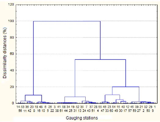
The complete linkage method presented easy interpretation of results and equal number of clusters for the three evaluated flows. For this method, the cut-off can be identified as the approximate distance of 19% of dissimilarity in a dendrogram, in which four groups are formed with homogeneous characteristics of flow for all the considered flows. In order to illustrate the achieved result, in Figures 1 and 2, the graphics of dissimilarity distance vs clustering steps and dendrogram for the variable Q7,10 are
each presented.
FIGURE 2. Dendrogram for Q7,10 showing the clustering steps from the furthest neighbor method.
By analyzing Figure 1, the first discontinuity is observed between the clustering steps 56 and 57. From this result, four hydrologically homogeneous regions were identified for the three analyzed flow characteristics, which followed the same performance through the application of clustering method (Figure 2).
MELO JÚNIOR et al. (2006) obtained good results with the complete linkage clustering method in studies of precipitation.
Homogeneous regions
Through the complete linkage clustering method, four regions with homogeneous characteristics of flow for the Doce river basin were obtained, as described:
Region I – composed of stations with smaller flows and drainage areas. Spatially comprised of headwater regions and small tributaries. Seventeen (17) gauging stations comprise this region for all studied flows with drainage areas varying from 166 to 970 km².
Region II – intermediate region between regions I and III, which were composed of 12 gauging stations with drainage areas varying from 757 km² to 1.396 km².
Region III – intermediate region between regions II and IV. Spatially constituting of the main tributaries of the greater flow rivers of the basin and comprised of 13 gauging stations with drainage areas varying from 1,200 to 3,055 km².
Region IV – comprised of stations with greater flows and drainage areas. Spatially constituted of the key channel of the Doce River and its main tributaries: Piracicaba, Santo Antônio, Suaçuí and Manhuaçu. Nineteen gauging stations comprise this homogeneous region with drainage areas varying from 2,578 to 81,940 km².
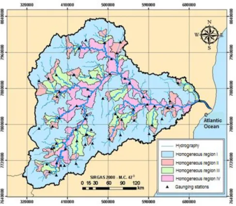
Figure 3 presents the spatial configuration of the four hydrologically homogeneous regions for the flows Q7,10, Q90 and Q95, that presented recurring hydrological performance. For the delimitation of
FIGURE 3. Hydrologically homogeneous regions for minimum streamflow obtained for the Doce river basin.
In analyzing Figure 3, it is noticed that the homogeneous region of greatest spatial scope is region I (headwater regions and smaller drainage areas), followed by region IV (channel of main river and main tributaries), region III and region II.
It is highlighted that drainage areas inferior to 160km² and superior to 82,000km² were included in the hydrological regions I and IV, respectively. However, it is important to emphasize that the major parts of the Doce river basin do not allow for adequate monitoring (drainage areas smaller than 160km²), thus requiring adoption of other criteria for result projections in these regions.
RIBEIRO et al. (2005) worked with minimum streamflow of reference (Q7,10, Q90 and Q95)
and obtained seven hydrologically homogeneous regions for the Doce River basin. MARQUES et al. (2009) investigated the same watershed and employed minimum streamflow of reference (Q7,10,
Q90 and Q95) in quarterly periods, obtaining hydrologically homogeneous regions.
It is highlighted that the regions the mentioned authors considered are subdivisions and/ or spatial junctions of hydrologically homogeneous regions found through the application of methodology presented in this study, based on unities of existing water resources management and sub-basins of the Doce River basin.
It is essential to distinguish that the methodology proposed in this study is based on multivariate statistical analysis and the obtained results point to the general hydrological performance of the Doce River basin.
The result obtained by the proposed methodology was complemented by the multiple regression analysis between the dependent variables (minimum streamflow characteristics) and the independent variables (climate and morphometric variables), to obtain regional equations for the four hydrologically homogeneous regions.
Multiple regression analysis
regression of linear, potential, exponential, logarithmic and reciprocate types were adjusted. Table 5 presents for each homogeneous region, the regression equations that adjusted best to the variables Q7,10, Q90 and Q95.
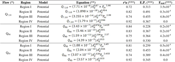
TABLE 5. Regression models that adjusted best to the minimum and average flow characteristics and the obtained adjustments.
Flow (*) Region Model Equation (**) r²a (***) E.P. (***) F0.05 (***)
Q7,10
Region I Potential 0.72 0.313 3.5x10⁻⁴
Region II Potential 0.82 0.491 0.3x10⁻⁴
Region III Potential 0.74 0.455 4.8x10⁻⁴
Region IV Potential 0.92 0.367 0.0
Q90
Region I Potential 0.84 0.228 0.2x10⁻⁴
Region II Potential 0.83 0.367 0.2x10⁻⁴
Region III Potential 0.75 0.364 4.2x10⁻⁴
Region IV Potential 0.93 0.330 0.0
Q95
Region I Potential 0.81 0.259 0.5x10⁻⁴
Region II Potential 0.82 0.453 0.4x10⁻⁴
Region III Potential 0.74 0.389 0.4x10⁻⁴
Region IV Potential 0.92 0.345 0.0
(*) Flows in m³ s-1 , A
d in km² and Psc in mm.
(**) Equations valid to the interval of independent variables of the gauging stations that constitute the hydrologically homogeneous region.
(***) adjusted determination coefficient (r²a ), the standard error of estimate (EP) and significance level of5% by the F test.
In order to meet the selection criteria of regression equations, it was necessary to exclude three gauging stations for region I (56570000, 56935000, 56993002) and one gauging station for region 4 (56880000).
By analyzing Table 5, it can be observed:
The regression model that adjusted best to the flow data was the potential. The same performance for the regional equations was achieved by RIBEIRO et al. (2005) and MARQUES et al. (2009) for the Doce River basin;
The most important independent variable for the study was drainage area (Ad) followed by
average semiannual rainfall in rainy season (Psc);
The regional equations presented for the four hydrologically homogeneous regions, defined by the methodology proposed in this study, showed determination coefficients higher than 0.70, standard errors of estimate lower than 0.5 and significance levels of 5% by the F test. The results achieved through multiple regression analysis were considered satisfactory, validating the scientific methodology presented in this study.
From previous knowledge of the region, the use of spatial analysis tools and the experience of an hydrologist, multivariate statistical analyses of both principal components and of clustering can contribute to the subdivision of hydrologically homogeneous regions, thus enabling more consistent decision-making, from a more reliable database (eliminating variables that contribute little to the study) of obtained clusters (verification of statistical performance of flow characteristics from the dendrogram).
CONCLUSIONS
Principal components analysis presented satisfactory results for excluding little representative variables in the identification of hydrologically homogeneous regions.
The first two principal components, Y1 eandY2, were responsible for 77.92% of data total
The Mahalanobis similarity matrix and the complete linkage clustering method demonstrated great results in the identification of hydrologically homogeneous regions for all studied flows.
Four hydrologically homogeneous regions were obtained for all studied minimum flow characteristics.
The regionalization equations obtained through multiple regression analysis for the minimum flow characteristics were considered satisfactory, validating the scientific methodology presented in this study.
The methodology proposed for identification of the number of homogeneous regions showed great results, enabling the elimination of subjectivity in the identification of hydrologically homogeneous regions.
ACKLOWDEGMENTS
The authors want to thank the Research Support Foundation of Minas Gerais state (FAPEMIG), the Coordination for the Improvement of Higher Education Personnel (CAPES), the National Council for Scientific and Technological Development (CNPq) and the Federal University of Viçosa (UFV) for the funding this study.
REFERENCES
ARRUDA, N. P.; HOVELL, A. M. C.; REZENDE, C. M.; FREITAS, S. P.; COURI, S.; BIZZO, H. R. Correlação entre precursores e voláteis em café arábica brasileiro processado pelas vias seca, semiúmida e úmida e discriminação através da análise por componentes principais. Química Nova, São Paulo, v. 35, n. 10, p. 2044-2051, 2012.
ARRUDA, N. P.; HOVELL, A. M. C.; REZENDE, C. M.; FREITAS, S. P.; COURI, S.; BIZZO, H. R. Discriminação entre estádios de maturação e tipos de processamento de pós-colheita de cafés arábica por microextração em fase sólida e análise de componentes principais. Química Nova, São Paulo, v. 34, n. 5, p. 819-824, 2011.
ASSANI, A. A.; CHALIFOUR, A.; LÉGARÉ, G.; MANOUANE, C.; LEROUX, D. Temporal regionalization of 7-day low flows in the St. Laurence watershed in Quebec (Canada). Water Resources Management, Dordrecht, v. 25, p. 3559-3574, 2011.
BELLOMARINO, S. A.; PARKER, R. M.; CONLAN, X. A.; BARNETT, N. W.; ADAMS, M. J. Partial least squares and principal components analysis of wine vintage by high performance liquid chromatography with chemiluminescence detection. Analytica Chimica Acta, Amsterdam, v. 678, p. 34-38, 2010.
CARVALHO, M. F.; ALBUQUERQUE JUNIOR, C. L.; GUIDOLIN, A. F.; FARIAS, F. L. Aplicação da análise estatística multivariada em avaliações de divergência genética através de marcadores moleculares dominantes em plantas medicinais. Revista Brasileira de Plantas Medicinais, Botucatu, v. 11, n. 3, p. 339-346, 2009.
CASTIGLIONI, S.; CASTELLARIN, A.; MONTANARI, A. Prediction of low-flow indices in ungauged basins through physiographical space-based interpolation. Journal of Hydrology, Amsterdam, v. 378, p. 272-280, 2009.
COUTO JR, C. G.; GALDI, F. C. Avaliação de empresas por múltiplos aplicados em empresas agrupadas com análise de cluster. Revista de Administração Mackenzie, São Paulo, v. 13, n. 5, p. 135-170, 2012.
FARO JR, A. C.; RODRIGUES, V. O.; EON, J.; ROCHA, A. S. Análise por componentes principais de espectros nexafs na especiação do molibdênio em catalisadores de hidrotratamento.
Química Nova, São Paulo, v. 33, n. 6, p. 1342-1347, 2010.
GUEDES, H. A. S.; SILVA, D. D.; ELESBON, A. A. A.; RIBEIRO, C. B. M.; MATOS, A. T.; SOARES, J. H. P. Aplicação da análise estatística multivariada no estudo da qualidade da água do Rio Pomba, MG. Revista Brasileira de Engenharia Agrícola e Ambiental, Campina Grande, v.16, n. 5, p. 558-563, 2012.
HATVANI, G. I.; KOVÁCS, J.; KOVÁCS, I. S.; JAKUSCH, P.; KORPONAI, J. Analysis of long-term water quality changes in the Kis-Balaton Water Protection System with time series, cluster
analysis and Wilk’s lambda distribution. Ecological Engineering, Amsterdam, v. 37, p. 629-635, 2011.
HELENA, B.; PARDO, R.; VEGA, M.; BARRADO, E.; FERNÁNDEZ, J. M.; FERNÁNDEZ, L. Temporal evolution of groundwater composition in an alluvial aquifer (Pisuerga River, Spain) by principal component analysis. Water Research, Amsterdam, v.34, p.807-816, 2000.
ISLABÃO, G. O.; PINTO, M. A. B.; SELAU, L. P. R.; VAHL, L. C.; TIMM, L. C.
Characterization of soil chemical properties of strawberry fields using principal component analysis. Revista Brasileira de Ciência do Solo, Viçosa, MG, v.37, n.1, p.168-176, 2013. JESUS, S. C.; EPIPHANIO, J. C. N. Sensoriamento remoto multissensores para a avaliação temporal da expansão agrícola municipal. Bragantia, Campinas, v. 69, n. 4, p. 945-956, 2010. JOLLIFE, I. T. Principal component analysis. 2. ed. Springer, 487 p., 2002.
MARQUES, F. A.; SILVA, D. D.; RAMOS, M. M.; PRUSKI, F. F. Sistema multi-usuário para gestão de recursos hídricos. Revista Brasileira de Recursos Hídricos, Porto Alegre, v.14, n.4, p.51-69, 2009. MELO JÚNIOR, J. C. F.; SEDIYAMA, G. C.; FERREIRA, P. A.; LEAL, B. G. Determinação de regiões homogêneas quanto à distribuição de freqüência de chuvas no leste do Estado de Minas Gerais. Revista Brasileira de Engenharia Agrícola e Ambiental, Campina Grande, v.10, n.2, p.408-416, Campina Grande, PB, 2006.
MISHRA, A. K.; COULIBALY, P. Hydrometric network evaluation for Canadian watersheds.
Journal of Hydrology, Amsterdam, n.380, p.420-437, 2009.
MWALE, D.; GAN, T. Y.; DEVITO, K. J.; SILINS, U.; MENDOZA, C.; PETRONE, R. Regionalization of runoff variability of alberta, canada, by wavelet, independent component, empirical orthogonal function, and geographical information system analysis. Journal of Hydrologic Engineering, New York, v.16, n.2, p.93-107, 2011.
CBH-Doce – Comitê da Bacia Hidrográfica do Rio Doce. Plano Integrado de Recursos Hídricos da Bacia do Rio Doce. Disponível em: < http://www.cbhdoce.org.br/documentos/pirh/plano-diretor-da-bacia-do-doce-pirh/>. Acesso em: mar. 2010.
REID, M. K.; SPENCER, K. L. Use of principal components analysis (PCA) on estuarine sediment datasets: The effect of data pre-treatment. Environmental Pollution, Barking, v.157, p.2275-2281, 2009.
RENCHER, A. C. Methods of multivariate analysis. 2th ed. Wiley-Interscience, 2002. 708p. RESENDES, A. P. C.; SILVEIRA, N. A. P. R.; SABROZA, P. C.; SOUZA-SANTOS, R.
Determinação de áreas prioritárias para ações de controle da dengue. Revista de Saúde Pública, São Paulo, v. 44, n. 2, p. 274-282, 2010.
SAMUEL, J.; COULIBALY, P.; METCALFE, R. A. Estimation of continuous streamflow in ontario ungauged basins: comparison of regionalization methods. Journal of Hydrologic Engineering, New York, v.16, n.5, p.447-459, 2011.
SILVA, S. F. R.; MATOS, D. C.; SILVA, S. L.; DAHER, E. F.; CAMPOS, H. H.; SILVA, C. A. B. Chemical and morphological analysis of kidney stones: A double-blind comparative study. Acta Cirúrgica Brasileira, São Paulo, v. 25, n. 5, p. 444-448, 2010.
SOUSA, H. T.; PRUSKI, F. F.; SOUSA, J. F.; BOF, L. H. N.; CECON, P. R. Sistema
computacional para regionalização de vazões – SisCoRV 1.0. Viçosa: Universidade Federal de Viçosa, 2008.
WILKS, D. S. Statistical methods in the atmospheric sciences. London: Academic Press, 2006. 630 p.