A Work Project, presented as part of the requirements for the Award of a Masters’ Degree in Finance from the NOVA - School of Business and Economics.
Pair Trading: Clustering Based on Principal Component
Analysis
Rafael Govin Cardoso, 664
A Project carried out on the Finance Master, under the supervision of: Professor Pedro Lameira.
2
Abstract
This study focuses on the implementation of several pair trading strategies across three emerging markets, with the objective of comparing the results obtained from the different strategies and assessing if pair trading benefits from a more volatile environment. The results show that, indeed, there are higher potential profits arising from emerging markets. However, the higher excess return will be partially offset by higher transaction costs, which will be a determinant factor to the profitability of pair trading strategies.
Also, a new clustering approach based on the Principal Component Analysis was tested as an alternative to the more standard clustering by Industry Groups. The new clustering approach delivers promising results, consistently reducing volatility to a greater extent than the Industry Group approach, with no significant harm to the excess returns.
3
1.
Introduction
If you would ask 100 traders if they know what pair trading is, 99 would say yes. This approach, where an investor benefits from a relative misprice between two securities, is one of the most well-known strategies across the financial industry. Despite its secretive nature, it is already possible to find several studies where scholars assess the impact of different methodologies1 in the strategy’s results. However, little importance has been given to two important factors: (1) the market where the strategy is implemented and (2) the clustering process of the stocks into groups. It is possible that, due to its classification as a contrarian strategy, more volatile markets would have a positive effect on the results. Also, while different methods to define the pairs have been exhaustively studied, there is room for improvement in the clustering process. For this reason, a pair trading strategy was tested in 3 different emerging (BRICS) countries: India, South Africa and Brazil. Special attention was given to the level of development of the financial markets of the countries, for the implementation of the strategy to be realistic. An innovation to the clustering process is also tested, using the Principal Component Analysis combined with Hierarchical Clustering to group stocks with similar risk profile. Finally, different pair trading strategies are compared and a sensitivity analysis undertaken to different parameters, to understand, nowadays, where the value of this strategy comes from.
Section 2 provides a theoretical contextualization of the subject, explaining the concept and intuition behind pair trading. The methodology adopted will be explained in section 3, followed by the data used in section 4. The results will be presented in the following section. Finally, the conclusion summarizes the main findings, followed by considerations and limitations that the reader must keep in mind.
1
Several approaches to define the pairs to be traded, the trading signal, the holding period, the hedge ratio, the entry and
4
2.
Theoretical Contextualization
Arbitrage
Arbitrage, the possibility to make a sure profit with no risk due to the mispricing of assets,is considered one of the main pillars of finance. Even though such opportunities are assumed absent by different economic and asset pricing models, hedge funds and investment banks still keep looking for the “golden pot at the end of the rainbow”. This can lead to two conclusions: (1) there are enough arbitrage opportunities to sustain the number of hedge funds trading, and (2) with this many arbitrageurs, most opportunities will not persist through time, as they are likely to be found by one of the market players.
Arbitrage can be divided in two types: pure (deterministic) arbitrage, and statistical (relative) arbitrage. The main difference is that while pure arbitrage benefits from relative mispricing of securities in a riskless way2, the statistical arbitrage is based on the expected value of the assets, bearing a certain amount of risk3. However, statistical arbitrage remains a very broad term, which can include strategies such as merger arbitrage, liquidation arbitrage and pair trading, among others. This type of arbitrage finds its root around the decade of 80, and it is considered an evolution from the simple strategy of pair trading.
Pair Trading
The intuition surrounding pair trading is misleadingly simple: find two stocks whose prices “move together” and when the relative price of the stocks deviates from the normal
2
Future against cash and triangular forex arbitrage are two examples of this kind of arbitrage.
3
Hogan et al. (2004) define statistical arbitrage as a zero initial cost self-financing trading strategy with cumulative
discounted value v(t) such that:
1. 0 = 0; 2. lim→ > 0; 3.lim→ < 0 = 0; and
5 level, enter a position, with the objective of profiting from an expected correction of the prices to the equilibrium level. So, when the spread between the stocks widens, the investor will “sell the winner and buy the loser”. For this reason, pair trading is included in the group of contrarian strategies, where an investor goes against the overall market trend, buying stocks performing poorly and selling stocks with a good performance.
There are two main theories explaining the excess return of these strategies, both of them backed by significant literature. The first theory defends that contrarian strategies are fundamentally riskier, with adjusted excess returns (Fama and French 1992). In response to this theory, Lakonishok, Shleifer and Vishny (1994) defend that the abnormal returns of contrarian strategies are not explained by a fundamentally higher risk, but by an overreaction of “naive” investors, overbuying/overselling well/bad performing stocks.
Depending on the refinements of the strategy, pair trading has characteristics that are important to refer: (1) it is self-financing, (2) it is market-neutral4 and (3) it focuses on the relative price of assets. By short-selling one stock and using the funds to buy another stock within the same market, the investor does not need initial capital to implement this strategy (self-financing). Besides, by buying and selling a stock, he will be hedged against market-wide fluctuations, since the net exposure will be null (market neutral).
Finally, and also very important, is that the value of the stocks is being analyzed in a relative perspective (and not absolute). According Gatev et al. (2006), relative pricing avoids the uncertainty and degree of error related to absolute methods and can be seen as a less restrictive application of the Law of One Price (LOP), which states that “two investments with the same payoff in every state of nature must have the same current
value” (Ingersoll, 1987). Moreover, relative pricing holds for recessions and booms of the economy, since the relative price can be correct, while the absolute is not.
4
6
History
The notion of statistical arbitrage was first introduced in the finance world around mid-1980’s, at Morgan Stanley. Nuno Tartaglia, a quant at this investment bank, hired and oversaw a group of mathematicians, physicist and computer scientists, in order to create quantitative strategies that would find and profit from arbitrage opportunities in the financial markets, using sophisticated statistical tools (Vidyamurthy 2004). The strategies developed were characterized by a strong analytical and quantitative perception of arbitrage (as opposed to the trader’s intuition) and were then implemented through automated trading systems, which were considered state of the art at the time. One of the first strategies developed was to look for stocks whose prices moved together and trade them when they diverged, in other words, pair trading.
As it turned out, this strategy delivered impressive results during the second half of the 1980’s, until the group5 split up in 1989. The members spread to other hedge funds and investment banks, taking with them the recent concept of statistical arbitrage. With the expansion of the strategy to hedge funds and investment banks all over the world, competition increased and profits became harder to achieve, leading to refinements and enhancements of the initial and simpler strategy of pair trading. Different approaches to define pairs that “move together” were tested, as well as clustering techniques and definitions of spread and deviation. To define these inputs, diverse tools and techniques from different areas were adopted, ranging from simple statistic measures to more developed mathematical techniques used in physics or neural networks study. Even though the amount of research about this topic increased in recent years, it remains a rather secretive topic, since hedge funds and other practitioners would be harming their profits by publishing their findings.
5
7
3.
Literature Review
One of the earliest and most cited papers was published in 1999 by Gatev et al. (1999). In this paper, a back-test of a simple pair trading strategy is performed, in order to assess its profitability. Stocks in the US market are paired according to the minimum distance in the historical normalized price space, and different trading rules are tested over the period from 1967 to 1997. The same strategy was applied to the stocks clustered by industries, to assess the consistency of the results across industries. The results show significant excess return, which are robust to transaction costs. Also, a simple mean reversion strategy is computed, showing that pair trading adds value to this simple strategy. This paper was reproduced by the same authors in 2006 (Gatev, Goetzmann and Rouwenhorst 2006) in order to assess if the strategy was still profitable, and as a way to avoid data-mining. The strategy was tested from 1967-2002 still with returns robust to transaction costs.
These papers were then used as a benchmark for two studies by Do and Faff in 2010 and 2012, to assess if the strategy remained profitable after the development of technology and financial markets, as well as with the widespread use of pair trading. In 2010 the strategy was extended to include data up to 2008, which revealed a declining trend in the profitability of the strategy. It was also shown that this was not due to overcrowding of the strategy or rise in hedge fund activity but due to less reliable convergence properties. The study was repeated in 2012, and it was found that, from 2002, it had become unprofitable.
In 2002, Alexander and Dimitriu (2002) published an important paper, where they used the cointegration concept to define which pairs to trade, as an alternative to the minimum distance of normalized price. The strategy was applied to the DJIA6, and showed very encouraging results, with robust returns, low volatility and negligible market correlation.
6
8 This new approach to define pairs was then largely used in different papers, such as Caldeira and Moura (2013), who successfully back-tested the strategy in the Brazilian market. Dunis et al. (2010) is another example where cointegration is used to define the pairs which will be traded under a high frequency perspective. In 2004, Vidyamurthy published a book7, where the cointegration approach is explained in detail and which is widely used as a benchmark by investors.
Another important reference in pair trading is the study published by Elliot et al (2005), who define a third approach to pair trading by looking at the spread as a mean-reverting Gaussian Markov process. However, there are few examples where this method is applied to real data. In 2010, Bogomolov compares the three above described methods (1) distance, (2) cointegration and (3) stochastic spread in Australia. After accounting for transaction costs, the strategies are shown to be unprofitable or with minimal profit.
The development of statistics and technology brought about more complex and computationally heavier methods, to be applied to statistical arbitrage and pair trading. One of the most important statistical tools is the Principal Component Analysis (PCA), which can be applied to many different areas, including pair trading. One of the first studies to include PCA in the context of statistical arbitrage was Avellaneda and Lee (2010), which used PCA to extract the risk factors of the stocks, in order to isolate the idiosyncratic noise. In a clustering perspective, however, PCA was only applied to Risk Portfolio Optimization (Alexander and Dimitriu 2005). Recently, high frequency (pair) trading has also been the object of attention, with different studies concluding that the strategy is very sensitive to the speed of execution (Bowen, Hutchinson and O’Sullivan 2010) and can be improved with high-frequency trading (Dunis, et al. 2010).
7
Vidyamurthy, Ganapathy. Pairs Trading: quantitative methods and analysis. Vol. 217. John Wiley & Sons,
9
4.
Data
The data used in this study consist of the closing prices (PX_LAST)8 of the stocks that constitute the major indexes of Brazil, India and South Africa, from the 1st of January 2003 until the 31st of December 2013. This dataset comprises around 2870 data points, on 3 emerging markets (BRICS countries), going back 11 years. For each of the companies, the sector of activity is also reported, according to the Global Industry Classification Standard (GICS), which divides companies in 10 sectors9.The following indexes were considered:
- BOVESPA: index that includes 50 of the most liquid companies traded in the São Paulo Stock, Mercantile and Futures Exchange, in Brazil.
- FTSE/JSE TOP40: index that includes the top 40 companies (by market capitalization) in the Johannesburg Stock Exchange, in South Africa.
- S&P BSE SENSEX: index including the top 30 companies by liquidity and depth, from all major industries of the Bombay Stock Exchange, India.
To avoid the problem of survivorship bias10, the companies used were the ones that constitute each of the indexes as from the 1st of January of 2003. Besides the closing prices, the volume of each trading day was also obtained for each company, to filter and exclude companies that are not liquid enough to be considered in the proposed strategy. All data was adjusted to dividends and stock splits, or else it would cause problems to the strategy, since the jumps in prices caused by dividends distribution and stock splits would give us misleading buy or sell signals.
8
All the data necessary was obtained from Bloomberg L.P. 9
Industry Groups according to GICS: Energy, Materials, Industrials, Consumer Discretionary, Consumer
Staples, Health Care, Financials, Technology, Telecommunication Services and Utilities.
10
10
5.
Methodology
The sequence of steps of the strategy will be explained in detail in this section. All necessary calculations were performed using the MATLAB11 software.
Data Filtering
The first step of the strategy involves the filtering of stocks, in order to avoid two main problems. First of all, since the stocks under consideration are the ones that constitute the respective indexes as from 200312, some might have gone bankrupt, been acquired or become private, being no longer available for investors. For this reason, at the end of each year (260 days), a rebalancing of the portfolio is undertaken, eliminating the stocks that ceased to exist as publicly traded companies. The second part of the filtering process involves the elimination of the less liquid stocks, since they add an extra risk to every strategy. Moreover, with less liquid stocks, the assumption that an investor can perform a trade without influencing the price of the stock becomes less realistic, thus jeopardizing the feasibility of the strategy. For this reasons, every year, the 10 percent (%) less liquid13 stocks of each index were not considered for the strategy.
Pair Formation
In order to define the co-movement of shares, the two most common methods in the literature were used: distance and cointegration approach.
•
Distance approach
The first approach, first used by Gatev et al. (1999) and since then extensively used in the literature, is the distance method. This method defines the co-movement of pairs as the
11
MATLAB and Statistics Toolbox Release 2014a, theMathWorks Inc. Natick, Massachusetts, United States.
12
To avoid survivorship biased.
13
11 squared distance of the normalized price series. The smaller the distance, the greater the co-movement of prices. The series of normalized prices for each stock is defined as the cumulative returns index. By construction the index begins at one (100%), and its value will change according to the subsequent returns.
= 0 1 + (
+3
With the normalized price series for each stock, the squared distance between each possible pair of stocks is computed.
4 5 67 = 8 6− 7
-*
+3
Using the distance obtained, the pairs are ranked and the ones with the smallest distance are selected. Every year (260 days), the distance between pairs will be recalculated and the pairs redefined. Since the indexes that are used for the purposed of this study comprise a limited amount of stocks (from 30 to 60), only the top 10 pairs will be used for the strategy. Once the pairs are obtained, the definition of spread, deviation, and the rules to open and close the position have to be decided upon. The spread was defined as the difference between the log prices, and the measure of deviation as the standard deviation of the spread. The rules to open a position are:
- Sell Spread (short-sell the first and buy the second stock of the pair):
:;(#<= > :;(#<=>>>>>>>>>>-/+ ?-/@ & A
- Buy Spread (buy the first and short-sell the second stock of the pair):
:;(#<= < :;(#<=>>>>>>>>>>-/− ?-/@ & A
12 between the pairs. To keep a dollar-neutral strategy (and approximately market neutral), the same dollar-amount is invested in both stocks. The exit rule will be very simple, and the position will be closed if the value of the spread is back between14
:;(#<= = B:;(#<=>>>>>>>>>>-/− 0,5 ∗ ?-/@ & A ; :;(#<=>>>>>>>>>>-/+ 0,5 ∗ ?-/@ & AF
•
Cointegration approach
The second approach, also widely used in the literature and first implemented by Alexander and Dimitriu (2002), is the cointegration approach. This concept was first introduced by Engle and Granger (1987) in order to model the relationship between integrated variables. If two variables are non-stationary, most of the simple estimation methods, such OLS, cannot be applied, as it violates some of its underlying assumptions15. Engle and Granger noticed that, although two variables are non-stationary, a linear combination of them can be stationary. If so, the variables are cointegrated and an error correction model16 can be created, and can be inferred using simple and standard statistical methods17, solving the problem at hand. In the years to follow, many adaptations and extensions of this model were proposed18.
As the idea behind pair trading is to find stocks that “move together”, the concept of cointegration perfectly suits the purpose, and can be used to define the pairs of stocks to be traded. In order to define the pairs, a cointegration test between every possible pair of stocks will be conducted, using the Engle-Granger (1987) two-step approach. In the first
14
This way, an investor will have a potential profit of 0.5 standard deviations of the Spread.
15
The expected value and variance of the variables must be constant and independent of time, which doesn’t happen
with integrated variables.
16
The error correction model will be stationary by construction.
17
Such as the Ordinary least squares (OLS) and Maximum Likelihood methods.
18
13 step, a possible cointegrated relationship is estimated by a simple regression of the following form.
Following the cointegration approach proposed by Chan (2013), the logarithm of prices was regressed with constant and no drift. Saving the residuals from the regression, the stationarity of the residuals19 was tested.
One important parameter of this test is the number of lags (p), which correspond to the level of autocorrelation of the residuals20. Since this parameter is unknown, the Akaike information criteria (AIC)21 will be used to decide to number of lags (Miao 2014).
Now, with all the inputs necessary, the ADF test will be performed, and if the null hypothesis is rejected, there are statistical reasons to believe that the residuals might be stationary, and the variables cointegrated. Once the Engle Granger two-steps approach is performed, the pairs are ranked according to the t-statistic obtained, and the ones with the lowest22 t-statistic are picked (Miao 2014). With the pairs defined, the spread between the stocks will now give the trade signals, using the coefficient from the initial regression23.
:;(#<=6,7 = log 6 − I6,7log 7 − J6,7
19
The method implemented was the Augmented Dickey Fuller method (ADF).
20
When choosing the number of lags, there is a tradeoff between the statistically validity of the DF test (if
autocorrelation arises, test is not valid), and the power of the test (degrees of freedom are lost with the increase of lag).
21
Other information criteria tests could be used, such as the Schwartz information criterion, the Hannan-Quinn criterion
or the Bayesian information criterion.
22
Since it is a one-tail test, the more negative the t-statistic of the regression of the residuals, the stronger is the
statistical rejection of the integration of the residuals.
23
Which makes the spread stationary.
∆L̂ = NL̂ ,3+ 8 O ∆L̂ , + !
+3
14 Following the same reasoning as in the distance approach, the same number of pairs,
enter and exit rules will be used. Once again, the pairs will be rebalanced every year.
Stock Clustering
Although pair trading is close to market neutral, there is still a great exposure to different risk factors. To reduce this exposure and the strategy’s volatility, several academics and practitioners cluster the stocks according to pre-defined risk factors24. In this study, two different clustering methods will be implemented: IG and PCA clustering.
•
Industry Groups
One of the most striking factors of risk can arise from the industries. If an investor has a large exposure to a certain industry, it can suffer heavy losses if a shock affects that same industry. For this reason, it is common to divide the stocks by industry, followed by a matching process into pairs. In the specific case of this thesis, the stocks are grouped according to the Global Industry Classification Standard (GICS) 10 sectors25.
•
Principal Component /Hierarchical clustering approach
Surprisingly, however, there is no further research aimed at finding other grouping processes, which could improve the results of the strategy. Despite delivering good results, clustering by industry groups is very restrictive and strict, and cannot be adapted to different samples. For this reason this study will clusters the stocks in a more flexible way, using two statistical tools: Principal Component Analysis and Hierarchical Clustering.
o Principal Component Analysis (PCA)
PCA is a tool widely used in diverse areas of study, mainly to simplify large quantity of data into a smaller and easier to understand data set. Basically, what PCA does
24
Most of the times, stocks are clustered according to Industry Groups (IG).
25
15 is to try to reduce the number of variables, keeping as much of the variability as possible. This is done by creating new variables (principal components), that are linear combinations from the original variables, but have the advantage of being uncorrelated by construction. The principal components are constructed in a way that the first component accounts for as much of the variance of the data as possible. Then, the second component will try to explain as much of the remaining variability as possible, and so on.
When computing PCA, two important outputs will be obtained: (1) the coefficients and (2) the scores. Taking “n” variables, the output will consist on “n” principal components, where each one can be written as a linear combination of the initial variables.
Q1 = R3S3 + R-S- + RTST + ⋯ RVSV
where “Z” stands for the normalized return of the stocks26, at each point of time (“i”). “ Q1 ” represent the scores, which will correspond to the data points of the new variables (principal components). Equally relevant, "R" represents the coefficient of each variable, which can be seen as the explanatory power that a certain PC has on the variable.
Making the bridge to the financial markets, by obtaining the principal components of a data set composed by a time series of stock returns, each principal component can be seen as representing a risk factor. The first component, which accounts for most of the variation of the data, is widely accepted as representing the market returns, while companies with similar coefficients related to the second component tend to be from the same industry (Avellaneda e Jeong-Hyun 2010). The further we advance in the components, the harder it is to link to a specific risk factor, since the explanatory power will substantially decrease and be less consistent across variables.
For the purpose of this study, a PCA will be computed for each of the indexes, and the stocks will be clustered based on the first two principal components obtained, since
16 they have a much stronger explanatory power than the following components27. This will, intuitively, create clusters of stocks that have similar exposure to the market returns and industry, in order to reduce the volatility of the strategy.
o Hierarchical Clustering Analysis (HCA).
Once the first two principal components and the coefficient of each stock are obtained, the stocks will be grouped employing the hierarchical clustering analysis. Initially, each cluster (one cluster for each stock) will be composed of one data point, with two dimensions (the two coefficients of each stock28, obtained with PCA). Then, HCA will compute the distance between each possible pair of data points, and join into a new cluster the two clusters with the smallest distance. Then, considering the new cluster obtained, the process will be repeated until the desired number of clusters is obtained.
In order to apply HCA, two inputs have to be defined: (1) distance metric and (2) linkage criteria. Several different distance metrics can be considered, but for the purpose of this study, the Euclidean Distance will be used29.
The linkage method defines how to compute the distance between clusters with more than one observation. The adopted criterion is the Average linkage clustering.
where “r” and “s” represent different clusters, “X " and "X$Y" represent the stocks that are a part of each cluster and “n”, the number of stocks in each cluster. Basically, the average
27
Explanatory power of Principal Components for each index for 2003 can be found in Figure A.1 of the Appendix.
28
Coefficients related to the first and second principal components, which will represent the explanatory power of these
components over each stock, and the risk exposure of each stock to the principal components (risk factor).
29
Where “n” stands for the number of dimensions of each cluster.
‖< − [‖ = \8 < − [ -V
+3
= (, 5 =] ]$1 8 8 = X ,X$Y V^
Y+3 V_
17 linkage will define the distance between two clusters as the average distance between their observations. The final results obtained from HCA are usually presented in the form of a dendrogram30, which gives a good visual representation of the results.
Compared with the clustering by Industry Groups, the advantage to use PCA/HCA is that it allows a clustering process considering simultaneously the exposure to several risk factors (the principal components). Furthermore, with this new approach, one can adapt the number of clusters to the data set and desired analysis. For the purpose of this study, since the number of stocks in each index is relatively small, 4 clusters will be created, in order to obtain enough stocks in each cluster to be able to match pairs that have a strong co-movement. In each cluster, 3 pairs will be defined31, using the minimum distance method. This method was chosen over the cointegration for two reasons: (1) it shows superior results when applied with no clustering (see next section for results) and (2) it is computationally less demanding. Once the pairs of each cluster are obtained, the same trading rules from the previous section will be applied. The process of clustering and matching pairs will be, once more, re-defined every year.
Mean-reverting returns
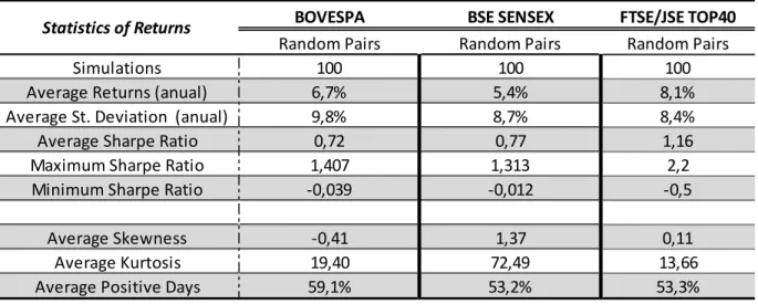
In order to assess if a pair trading strategy adds any value to a simple mean-reversion strategy, the process implemented by Gatev et al. (2006) was followed in this study. Each year, 10 pairs were randomly matched from each index, and the exact same trading rules and spread/trigger parameters were applied as in the distance approach. One hundred (100) simulations of this process were repeated and the results were then compared with the ones obtained from the distance and cointegration strategies.
30
A dendrogram for each index can be found in Figure A.2 of the Appendix.
31
The number of possible pairs to be traded is now 12. When using the HCA, if one stock presents abnormal
coefficients, it will be a cluster by itself, and no pairs will be traded in that cluster. Such situations are not uncommon, so
18
Transaction costs and calculation of returns
In mean-reverting strategies, a great deal of the profits can arise from the bid-ask bounce (Asparouhova, Bessembinder e Kalcheva 2010). Also, arbitrage opportunities are only profitable if the transaction costs, such as brokerage fees and bid-ask spread, are lower than the potential profit from the misprice of securities. However, for the indexes under consideration in this study, the official closing prices reported by the Stock Exchanges are either the price obtained from an auction or a VWAP (Volume Weighted Average Price)32. In both these situations, it is realistic to say that one can realize the trade at the reported price, and the bid-ask spread problem will not arise. For this reason, the strategy will only be adjusted to consider the brokerage fees, at a value of 0.15%33.
The calculation of the returns is usually a simple procedure, where the return represents the cash flows as a proportion of the initial capital invested. However, since pair trading is self-financing (no initial capital required), the returns’ calculation is not trivial. In order to compute the returns, the method used by most of the literature will be followed, which consists on dividing the payoff of each period by the total amount of pairs34. Since pairs will not trade every day, this is a conservative calculation of returns, as hedge funds are unlikely to “sit on the money” from the pairs that are not traded. Also, due to the market-neutrality of the strategy35, the returns can be seen as excess returns.
Sensitivity Analysis
Finally, in order to have a better understanding of where the value of this strategy comes from, a sensitivity analysis was performed, for the PCA clustering strategy.
32
A full description of the method to define the closing price of each Stock Exchange can be found in the corresponding
website of Johannesburg Stock Exchange, Bombay Stock Exchange and BM&F BOVESPA.
33
After researching about the brokerage fees, the lower bound of the fees applied to investors (0.15% per transaction)
will be used, as it is a realistic value for market players such as hedge funds and institutional investors.
34
This can be seen as a measure of return on committed capital, rather than return on the employed capital.
19 Different values were given to the rebalancing frequency, the spread average and standard deviation look back period, the transaction costs, and the principal components used in the clustering process, and the impact on the results36 was assessed.
6.
Results
Cointegration versus Distance Approach
First, the cointegration and distance approach were implemented to the three indexes under consideration (SENSEX, JSE and BOVESPA). The descriptive statistics of the results obtained can be found in the next table.
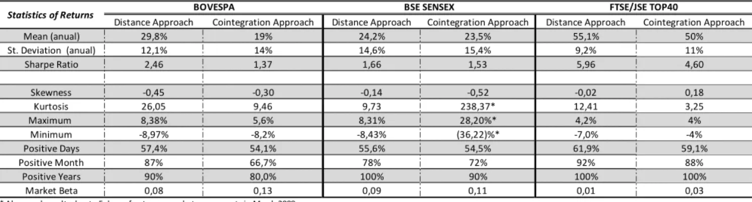
Table 1-Statistic of the Returns from the Distance and Cointegraton approaches.
The results show that both methods produce significant excess returns, with relatively low volatility, pointing to the possibility of a profitable strategy. India and Brazil show average returns between 20%-30%, with higher returns and lower volatility in the later, leading to a significantly better Sharpe Ratio. The distribution of the returns is also similar between these countries with a low skewness but high kurtosis, meaning that extreme events are likely to happen. Also, both countries show around 55% of days with positive excess return. South Africa, however, shows very promising results, with average excess returns close to 50%, lower volatility, and better behaved distribution of the returns. The number of positive days also increases to 60%. The correlation with the
36
Impact on results considered to be impact on Sharpe Ratio.
Distance Approach Cointegration Approach Distance Approach Cointegration Approach Distance Approach Cointegration Approach
Mean (anual) 29,8% 19% 24,2% 23,5% 55,1% 50%
St. Deviation (anual) 12,1% 14% 14,6% 15,4% 9,2% 11%
Sharpe Ratio 2,46 1,37 1,66 1,53 5,96 4,60
Skewness -0,45 -0,30 -0,14 -0,52 -0,02 0,18
Kurtosis 26,05 9,46 9,73 238,37* 12,41 3,25
Maximum 8,38% 5,6% 8,31% 28,20%* 4,2% 4%
Minimum -8,97% -8,2% -8,43% (36,22)%* -7,0% -4%
Positive Days 57,4% 54,1% 55,6% 54,5% 61,9% 59,1%
Positive Month 87% 66,7% 78% 72% 92% 88%
Positive Years 90% 80,0% 100% 90% 100% 100%
Market Beta 0,08 0,13 0,09 0,11 0,01 0,03
* Abnormal results due to 5 days of extreme market movements in March 2008.
*Excluding these days, one obtains a Kurtosis of 23,02, Maximum Return of 12,5%, Minimum Return of -10,3% and Sharpe Ratio of 1,40
FTSE/JSE TOP40 BSE SENSEX
BOVESPA
20 market37 is quite low in all indexes, due to the market neutral profile of pair trading. When comparing the results with the ones recently obtained in developed markets (Bogomolov 2010; Do and Faff 2012) one can see that more volatile markets benefit a pair trading strategy, with higher potential profits to be exploited.
Comparing both methods, the results show that the distance approach consistently outperforms the cointegration approach, mainly due a lower volatility. Both of the approaches show low skewness, high kurtosis and a strong proportion of positive days. These conclusions are in line with the results found in Australia (Bogomolov 2010), with the cointegration approach underperforming the distance approach.
Clustering Methods
The next step consisted on clustering the stocks38 with two different methods: the IG and the PCA approach. The results obtained are summarized in the following table.
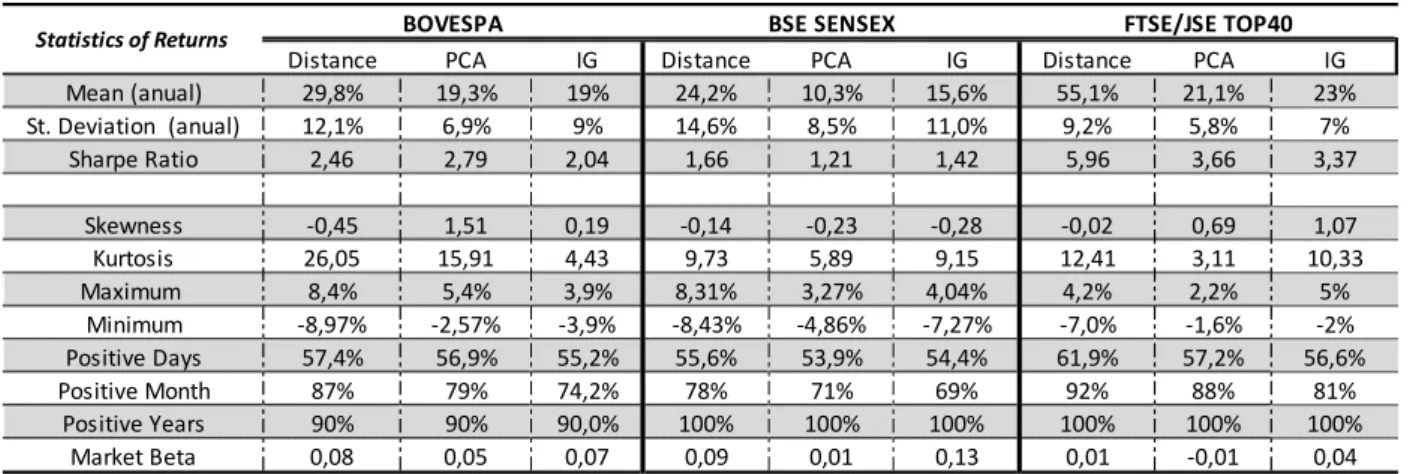
Table 2-Statistic of the Returns from the Distance, PCA and IG approaches.
The first conclusion arising is that, as expected, the clustering of the stocks significantly reduces the volatility of the strategy, to values between 5%-10%. However, the average excess returns also fell significantly, and the impact in the Sharpe Ratio is not consistent across the 3 countries. The clustering process will also have a significant impact
37
Measured by the “Beta”
38
Before applying the distance approach to pair the stocks.
Distance PCA IG Distance PCA IG Distance PCA IG
Mean (anual) 29,8% 19,3% 19% 24,2% 10,3% 15,6% 55,1% 21,1% 23%
St. Deviation (anual) 12,1% 6,9% 9% 14,6% 8,5% 11,0% 9,2% 5,8% 7%
Sharpe Ratio 2,46 2,79 2,04 1,66 1,21 1,42 5,96 3,66 3,37
Skewness -0,45 1,51 0,19 -0,14 -0,23 -0,28 -0,02 0,69 1,07
Kurtosis 26,05 15,91 4,43 9,73 5,89 9,15 12,41 3,11 10,33
Maximum 8,4% 5,4% 3,9% 8,31% 3,27% 4,04% 4,2% 2,2% 5%
Minimum -8,97% -2,57% -3,9% -8,43% -4,86% -7,27% -7,0% -1,6% -2%
Positive Days 57,4% 56,9% 55,2% 55,6% 53,9% 54,4% 61,9% 57,2% 56,6%
Positive Month 87% 79% 74,2% 78% 71% 69% 92% 88% 81%
Positive Years 90% 90% 90,0% 100% 100% 100% 100% 100% 100%
Market Beta 0,08 0,05 0,07 0,09 0,01 0,13 0,01 -0,01 0,04
BOVESPA BSE SENSEX FTSE/JSE TOP40
21 on the distribution of the returns, which are much better behaved when comparing with a no clustering strategy, with a reduction of both the skewness and kurtosis. The correlation with the market also points to an improvement of the strategy, mainly when clustering by PCA, with a smaller “Market Beta” across all indexes, with values below 0.05.
When comparing both clustering methods, the PCA approach is clearly able to reduce the volatility of the strategy to a larger extent than the IG approach. This will be followed by a reduction in the excess returns, which in Brazil and South Africa is not enough to offset the reduction in volatility, resulting in a higher Sharpe Ratio when compared to the IG clustering method. Only in India the reduction in excess returns will offset the lower volatility, leading to a lower Sharpe ratio. The distribution of excess returns is quite similar between these two methods, with the IG method presenting a kurtosis slightly lower. However, one must keep in mind that a very simple and rudimental PCA/HCA clustering was performed, which leaves room for improvement, since it can be adapted and personalized to different data sets.
Mean-Reverting Strategy
Following the reasoning by Gatev et al. (2006), this study assessed if the superior results obtained are simply due to a higher performance of mean-reverting strategies in more volatile markets, or if pair trading brings value to a simple mean reverting strategy. If no significant difference arises between the results of the 10 randomly matched pairs and the results from the distance and cointegration method, then there is evidence that the results are due to a better performance of mean-reverting strategies on these markets.
22 the returns from the mean reverting strategy are divided by four when compared to the pair trading strategies, adding significant value to the Sharpe Ratio and overall strategy.
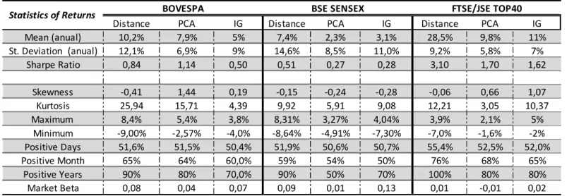
Impact of Transaction Costs
After adjusting the strategy for the transaction costs, the excess returns significantly decrease. Since the volatility remains similar, the high transaction costs of emerging markets will destroy a great portion of the profitability, with a strong negative impact on the Sharpe ratio. This can also be seen by looking at the proportion of positive days, which will fall to values close to 50%. The distribution of the returns will barely be affected, and the market correlation will remain close to null. A full description of the results can be found in Table A.2 in Appendix.
Sensitivity Analysis
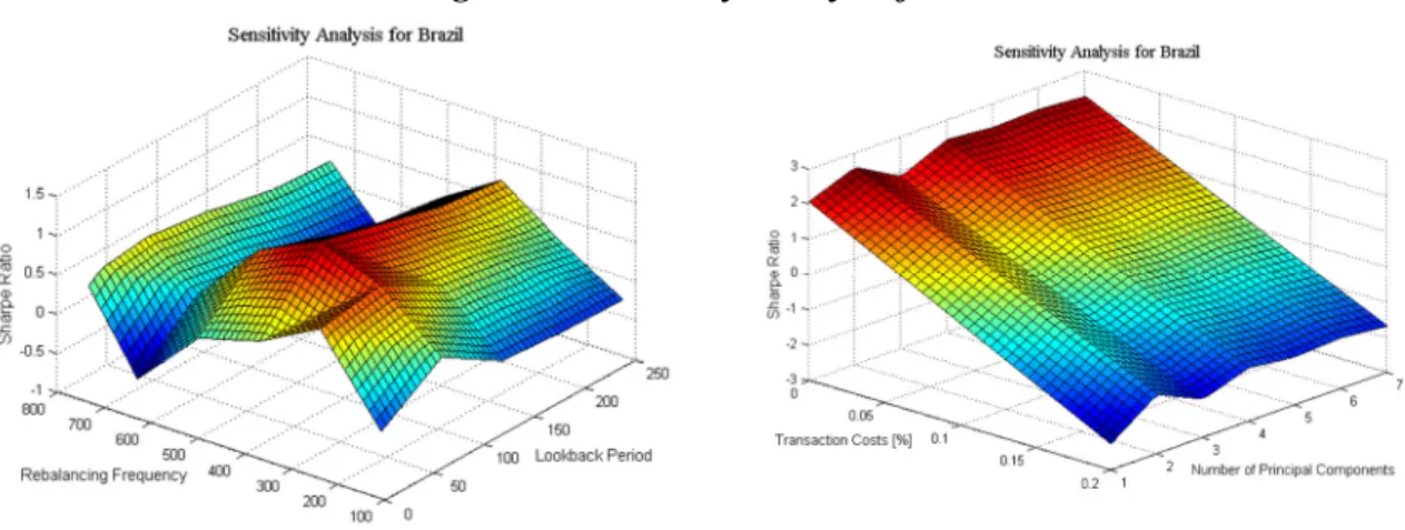
The results of the sensitivity analysis for Brazil39 can be found in the following figure.
Figure 1-Sensitivity Analysis for Brazil40
From the sensitivity analysis, some conclusions about the effect of the different inputs on the final Sharpe Ratio can be taken. First, as expected, the transaction costs will have a very strong effect, which can be the decisive factor between a profitable and unprofitable
39
Sensitivity Analysis for India and South Africa can be found in Figure A.4 of the Appendix.
40
23 strategy. However, variations on the number of PC on which the clustering will be based upon have a small impact in the final results, with a slight outperformance of a lower number of PC. Replicating the same analysis for India and South Africa (Figure A.4 of the Appendix), the conclusions are consistent with the ones on Brazil, for these two inputs. Focusing on the look back period, it shows a maximum positive impact on the Sharpe Ratio for values between 2 and 3 months (40-60 days), across the three markets. However, the rebalancing frequency does not have a consistent impact across countries. While in Brazil a maximum Sharpe ratio is obtained with a re-definition of pairs every two years, India benefits from a much faster rebalancing (130 days). On the other hand, South Africa shows better results when rebalancing the pairs less frequently (every 3 years).
7.
Conclusion
In this study different pair trading strategies were applied to 3 emerging markets with the following objectives: (1) assess such strategies in a more volatile environment (2) test a new clustering approach and (3) analyze where the value from pair trading comes from.
Based on the results, it is possible to conclude that more volatile environments bring higher potential returns when compared to more developed markets, benefiting the strategy. When comparing the cointegration with the distance method, the latter delivers a superior performance, due to a combination of lower volatility with higher returns. The pairs to be traded were also randomly matched, showing that pair trading adds value when compared to a simple mean-reverting strategy, increasing the excess returns.
24 might be beneficial, if the investor is willing to sacrifice some returns in exchange for a less risky and better behaved strategy. It was also found that the PCA clustering approach presents, in two out of three markets, a better Sharpe Ratio when compared to the IG clustering and consistently shows a lower volatility. Considering that a simple approach of the PCA was adopted, which can be adapted and optimized for the different markets, the results are evidence that this clustering processhas the potential to be successfully applied to pair trading and other strategies.
The transaction costs, however, will destroy a great deal of the profitability, eating away most of the returns, to values between 5%-10%. Even though the potential profits are higher in more volatile markets than developed markets, higher transaction costs will partially offset these profits. At the end of the day, transaction costs will be the determinant factor on the feasibility of the strategy, a conclusion that is corroborated by the sensitivity analysis. An individual investor with high transaction costs will have difficulty to generate enough returns to support the costs. However, a hedge fund with low costs can easily attain good returns at a relatively low risk from this strategy.
Finally, the sensitivity analysis also shows that the pair trading strategies will benefit if the spread mean and standard deviation are evaluated from a short-term perspective (2-3 months). However, the impact of the rebalancing frequency will be different across countries, meaning that no universal conclusion can be drawn.
8.
Other considerations
25 consider the possibility of higher transaction costs, and restrictions to short sell, which will have a strong impact on the results (Pizzutilo 2013). The implementation of the strategy on emerging markets also brings an extra consideration, since one is less familiarized with these markets. Even though the transaction costs were accordingly adjusted, one cannot exclude the possibility that different institutional settings (legislation, taxes, restriction on short selling, among other factors) might influence the strategy.
One must also not forget that, notwithstanding the fact that the strategy shows low volatility, it is not without significant risks. The 2007 crisis, which presented unprecedented losses for long/short hedge funds (Khandani and Lo 2007), is an evidence of that. Finally, any strategy is vulnerable to data mining, implying poorer results in the future, despite that the strategy was tested with simple and not optimized rules and inputs.
26
References
Alexander, Carol, and Anca Dimitriu. "Sources of Over-Performance in Equity Markets: Mean Reversion, Common Trends and Herding." ISMA Center, University of Reading (ISMA Center, University of Reading), 2005.
Alexander, Carol, and Anca Dimitriu. "The Cointegration Alpha: Enhanced Index Tracking and Long-Short Equity Market Neutral Strategies." ISMA Discussion Papers in Finance 8 (2002).
Asparouhova, Elena, Hendrik Bessembinder, and Ivalina Kalcheva. "Liquidity biases in asset pricing tests." Journal of Financial Economics 96, no. 2 (2010): 215-237.
Avellaneda, Marco, and Lee Jeong-Hyun. "Statistical arbitrage in the US equities market."
Quantitative Finance 10, no. 7 (2010): 761-782.
BM&F BOVESPA The New Exchange. n.d. http://www.bmfbovespa.com.br/ (accessed 12 2014).
Bogomolov, Timofei. "Pairs Trading in the Land Down Under." Finance and Corporate Governance
Conference. Bundoora, Australia, 2010.
Bowen, David, Mark C. Hutchinson, and Niall O’Sullivan. "High Frequency Equity Pairs Trading: Transaction Costs, Speed of Execution and Patterns in Returns." The Journal of Trading 5, no. 3 (2010): 31-38.
BSE Experience the new. n.d. http://www.bseindia.com/ (accessed 12 2014).
Caldeira, João Frois, and Guilherme Valle Moura. "Selection of a Portfolio of Pairs Based on Cointegration: A Statistical Arbitrage Strategy." Brazilian Review of Finance 11, no. 1 (2013): 49-80.
Chan, Ernie. Algorithmic trading: Winning Strategies and their Rationale. Vol. 625. John Wiley & Sons, 2013.
Do, Binh, and Robert Faff. "Are Pair Trading Profits Robust to Trading Costs?" The Journal of
Finance 35, no. 2 (2012): 261-287.
Do, Binh, and Robert Faff. "Does Simple Pairs Trading Still Work?" Financial Analysts Journal, 2010: 83-95.
Dunis, Christian L., Gianluigi Giorgioni, Jason Laws, and Jozef Rudy. "Statistical Arbitrage and High-Frequency Data with an Application to Eurostoxx 50 Equities." Liverpool Business
School, Working paper, 2010.
Elliot, Robert J., John Van Der Hoek, and William P. Malcolm. "Pairs Trading." Quantitive Finance
27 Engle, Robert F., and C.W.J. Granger. "Co-Integration and Error Correction; Representation,
Estimation and Testing." Econometrica: Journal of the Econometric Society 55, no. 2 (1987): 251-276.
Fama, Eugene F., and Kenneth R. French. "The Cross-Section of Expected Stock Returns." The
Journal of Finance 47, no. 2 (1992): 427-465.
Gatev, Evan G., William N. Goetzmann, and K. Geert Rouwenhorst. "Pairs Trading: Performance of a Relative Value Arbitrage Rule." National Bureau of Economic Research, Inc. 7032 (1999).
Gatev, Evan, William N. Goetzmann, and K. Geert Rouwenhorst. "Pairs Trading: Performance of a Relative Value Arbitrage Rule." Review of Financial Studies 19, no. 3 (2006): 797-827. Hogan, Steve, Robert Jarrow, Melvyn Teo, and Mitch Warachka. "Testing Market Efficiency Using
Statistical Arbitrage with Applications to Momentum and Value Strategies." Journal of
Financial economics 73, no. 3 (2004): 525-565.
Ingersoll, Jonathan E. Theory of Financial Decision Making. Vol. 3. Rowman & Littlefield, 1987. Johansen, Søren. "Statistical Analysis of Cointegration Vectors." Journal of Economic Dynamics
and Control 12, no. 2 (1988): 231-254.
JSE. n.d. https://www.jse.co.za/ (accessed 12 2014).
Khandani, Amir E., and Andrew W. Lo. "What Happened to the Quants in August 2007? Evidence from Factors and Transactions Data." Journal of Financial Markets 14, no. 1 (2011): 1-46. Lakonishok, Josef, Andrei Shleifer, and Robert W. Vishny. "Contrarian Investment, Extrapolation,
and Risk." The Journal of Finance 49, no. 5 (1994): 1541-1578.
Miao, George J. "High Frequency and Dynamic Pairs Trading Based on Statistical Arbitrage Using a Two-Stage Correlation and Cointegration Approach." International Journal of Economics
and Finance 6, no. 3 (2014): 96.
Pizzutilo, Fabio. "A Note on the Effectiveness of Pairs Trading For Individual Investors."
International Journal of Economics and Financial 3, no. 3 (2013): 763-771.
28
Appendix
Figure A.1-Explanatory power of the 25 first Principal Components
Figure A.2-Dendrogram for each of the indexes for 2003
29
Table A.1-Statistic of the Average Returns of the 100 Random Pairs Simulations
Figure A.3- Cumulative Returns of the 100 simulations
BOVESPA BSE SENSEX FTSE/JSE TOP40
Random Pairs Random Pairs Random Pairs
Simulations 100 100 100
Average Returns (anual) 6,7% 5,4% 8,1%
Average St. Deviation (anual) 9,8% 8,7% 8,4%
Average Sharpe Ratio 0,72 0,77 1,16
Maximum Sharpe Ratio 1,407 1,313 2,2
Minimum Sharpe Ratio -0,039 -0,012 -0,5
Average Skewness -0,41 1,37 0,11
Average Kurtosis 19,40 72,49 13,66
Average Positive Days 59,1% 53,2% 53,3%
30
Table A.2-Statistic of the Returns from the Distance, PCA and IG approaches, after Transaction Costs
Figure A.4-Sensitivity analysis for India and South Africa41
41
Where “Lookback Period” stands for the look back period used to calculate the Spreads’ mean and standard deviation, “Rebalancing Frequency” stands for the number of days after which the pairs are re-defined, “Number of Principal Components” stands for the number of PC used in the clustering process, and “Transaction Costs” for the Transaction Costs of each trade.
Distance PCA IG Distance PCA IG Distance PCA IG Mean (anual) 10,2% 7,9% 5% 7,4% 2,3% 3,1% 28,5% 9,8% 11% St. Deviation (anual) 12,1% 6,9% 9% 14,6% 8,5% 11,0% 9,2% 5,8% 7%
Sharpe Ratio 0,84 1,14 0,50 0,51 0,27 0,28 3,10 1,70 1,62
Skewness -0,41 1,44 0,19 -0,15 -0,24 -0,28 -0,06 0,66 1,07 Kurtosis 25,94 15,71 4,39 9,92 5,91 9,08 12,21 3,05 10,37 Maximum 8,4% 5,4% 3,8% 8,31% 3,27% 4,04% 3,9% 2,1% 5%
Minimum -9,00% -2,57% -4,0% -8,64% -4,91% -7,30% -7,0% -1,6% -2% Positive Days 51,6% 51,5% 50,4% 51,9% 50,6% 50,7% 55,4% 52,5% 52,0%
Positive Month 65% 64% 60,0% 59% 54% 50% 76% 68% 65%
Positive Years 90% 80% 70,0% 90% 50% 70% 100% 80% 80%
Market Beta 0,08 0,04 0,07 0,09 0,01 0,13 0,01 -0,01 0,02
BOVESPA BSE SENSEX FTSE/JSE TOP40