A Work Project, presented as part of the requirements of the Award of the Masters
Degree in Economics from the Nova School of Business and Economics
Compensating Variation and the Young Portuguese
Emigrants:
A Study on how to keep our own.
Manuel Maria Zuzarte Reis Piedade
Masters in Economics nº 609
A project carried out on the area of Microeconomics under the supervision of:
Professor Pedro Pita Barros
1
Compensating Variation and the Young Portuguese Emigrants:
A Study on how to keep our own.
ABSTRACT
Emigration has been a very present word in Portugal. Due to the effects of the
Economic Crisis and the Memorandum of Understanding policies, we have
witnessed a significant yearly migration outflow of people searching for better
conditions. This study aims to measure the factors affecting this flow as well as how
much the probability of emigrating has evolved during the years bridging 2006 to
2012. I shall consider the decision of emigrating as Discrete Choice Random Utility
maximization use a conditional Logit framework to model the probability choice for
31 OECD countries of destination. Moreover I will ascertain the compensating
variation required such that the probability of choice in 2012 is adjusted back to
2007 values, keeping all other variables constant. I replicate this exercise using the
unemployment rate instead of income. The most likely country of destination is
Luxembourg throughout the years analyzed and the values obtained for the CV is of
circa 1.700€ in terms of Income per capita and -11% in terms of the unemployment
rate adjustment.
2
1. INTRODUCTION
The Portuguese People have, historically, a propensity to emigrate. As a small yet quite
open economy, emigration dates as far back as the XV century, with the pioneers in the
Discoveries searching for fame and fortune around the World. Recently this has been
viewed as an adverse effect of the European Economic Crisis and a consequence of the
Memorandum of Understanding signed in 2011. With the deterioration of key aspects in
the Portuguese Economy – when comparing to other countries–, it is not surprising that
we might have witnessed a change in the Probabilities of Choice when deciding to
migrate or not as well as a change in the Probabilities of Choice for the countries
considered. This study’s core consists on the modeling of these Probabilities of Choice,
via a Conditional Logit models such as the one employed by Greenwood et. all (2001).
Given the nature of the Logit model we can apply the concept of Compensating
Variation to the Probabilities of Choice (de Palma, Killani, 2009) and calculate what
amount should be given to an individual such that his probabilities of choice are
adjusted to the ex-ante values. In this case it would be interesting to bring back the
probabilities’ values to pre-troika years.
I condition the probability of choice on the values of the explanatory variables for each
year and calculate the subsequent probability. This means that, given the parameters
estimated, I will be able to calculate for Norway–, conditional on the values that the
explanatory variables present for this country in particular on a given year–, what was
the probability of choosing this country as the Destination for an individual who is
deciding on the place to go to. Given that this calculation is done on a yearly basis, the
probabilities will evolve as the variables evolve. This is not surprising and we can
3
is relatively worse comparing to the Destination. For example, if Portugal’s Income per
capita decreases and Germany’s is kept constant from one year to the other, all else
being equal we can expect that the probability of choosing Germany will increase.
Regarding how the individual characteristics of the decision maker are approached, I
will follow the work of Greenwood et.all (2001) and impose two additional restrictions
on the model. Firstly I will focus on the effect of choice-specific attributes on the
migration decision and observe how the characteristics of a country affect the
individual’s destination choice. This model is not able to identify the individual
characteristics, as opposed to a Multinomial Logit for example which incorporates
individual characteristics on the decision making process, yielding different parameters
for different choices. There would be a great computation cost in terms of the number
parameters when incorporating individual characteristics and I do not have individual
level data, as such I will not employ this approach. Secondly, given that the conditional
Logit cannot identify directly the effects of individual characteristics, I will incorporate
relative measures between Portugal and the destination. This seems to meet the notion
of comparing countries when deciding to migrate, and the characteristics of specific
country should be thought f as of a proxy for an individual characteristic in the sense
that individuals will view differently the characteristics of a country. For example, a
high income individual will not consider the income per capita like a low income
individual.
This paper is organized as follows: in Section 2. I will review the literature; in Section
3. I will describe the methodology employed; in Section 4. I will present and discuss the
results; Section 5. I will conclude. The Annex will consist of complementary tables and
4
2. LITERATURE REVIEW
The study of migration flows has been quite vast and has carried out many paths in the
literature. As one may imagine, the implications of migration in a country are immense
and visible in many aspects of the society. They can range from economic issues such
as the equilibrium of the labor market to the impact in the productivity, the effect on
wages and long run sectoral bias, to social and cultural issues such as the integration of
migrant populations, the effect on crime, on social services costs, etc. In fact, Hooge et.
Al (2008) center the economic literature to explain migration in three theories:
economic and labor-based, where the factors boosting migration are connected to Standards of Living indicators, such as Income per capita, Unemployment rate, GDP
growth among others, and the decision is based on the relative measure between Origin
and Destination countries; cultural and hegemonic theories, where the factors are related to language and culture similarities, and a flow periphery-to-core is assumed;
social theories, where the factors are mainly the so called network effect, or the effect of
friends and family already established in the Destination or possessing some sort of
information, influencing the decision of the individual as to where to go and if he
should or not. This particular study will undergo the first road and hence I will base my
rational for migrating on economic and labor-based factors. It is common ground in migration models to refer to the Roy model (1951) to mathematically explain the
incentives to migrate, which was further adapted to the labor market and migration
modeling by Borjas (1987) where he builds the notion of comparing Origin and
Destination when deciding to migrate in terms of potential earnings. This is interesting
because it should be close to what an individual thinks when taking the decision of
5
attractive enough compared to the advantages of staying, given that there are associated
costs of moving.1 To this idea that the individual will compare aspects between the
Destination and the Origin and base his decision accordingly, many authors have
extended the notion of indicators. They need not to be only wages, income or wealth,
but also other components of an economy can be taken into consideration. Otrachsenko
and Popova (2013) investigate the effect of Life Satisfaction, using the Eurobarometer
Survey 27, for migration flows in Central and Eastern European countries and state that
people have greater intention to move when dissatisfied with life and that
socioeconomic and macroeconomic variables affect indirectly this decision through
their influence in life satisfaction. Stark (2005) studies the relation between income
inequality and the incentive to migrate, reaching the conclusion that a higher total
relative deprivation2 leads to higher incentives to migrate –given a constant income
level and that deprivation is positively correlated with the Gini coefficient– and hence
this measure of inequality is positively correlated with migration holding income
constant. Finnie (2004) posed the question “who moves?” to analyze the
inter-provincial migration in Canada by using panel data for tax fillers from the LAD dataset,
that collects detailed information on income, taxes, demographic characteristics such as
the province of residence. The author uses a Logit model to compute the probability of
moving from one province to another (by setting the dependent variable as whether or
1
According to this stream, the equation that models migration is: , where the decision to migrate of individual “i” ( ) is conditioned by the difference between the wage he receives in the destination country ( and the origin country , sustracting the cost of migrating ) and the personal loses of the migrant ( ).
2
6
not the individual’s province of residence changed from one year to another) as a
function of “environmental” factors such as the current province of residence, the
provincial unemployment rate and the area size, personal characteristics such as
language, age, marital situation and presence of children, key labor market indicators
such as earnings, receipt of unemployment insurance and social assistance. Their
analysis is performed for a span of circa 13 years and allows such detail mainly due to
the nature of the dataset.3 Similarly, Greenwood, Li and Davies (2001) also use a Logit
model applied to the inter-state migration in the United States of America for the years
of 1986 to 1997. The usage of panel data is particularly interesting as it captures time
effects that static analyses cannot do. The authors investigate the responses to relative
economic performance measurements, modeled by ratios between destination and origin
locations for income per capita and unemployment rate, and to the cost of moving,
modeled by the distance between locations. They also employ a fixed effects framework
to capture unobserved factors such as amenities and finally undertake a study on the
trade-off between variables that their model controls for. For instance, they compute the
unemployment rate – per capita income trade-off which is, as the authors calculate it,
the change in the destination Income pc required to offset an increase in the
unemployment rate. It can be seen as a Compensating Variation for unemployment
increases, since the econometrical model is solidly founded in Discrete Choice Theory
and derive from an individual’s utility maximization (McFadden 1973). This particular
paper will be the main reference for this WorkProject and I will derive to a similar
model, however directed at the emigration from Portugal to other countries.
3
7
3. METHODOLOGY
Database description
The data used in this Work Project is comprised of Inflows of Portuguese population,
income per capita, unemployment rate, GDP growth factor4 and distance for 31 countries in the OECD. This data selection is compiled for 6 years, from 2006 to 2012,
and follows the literature set up such as Greenwood et. al (2001) and Finnie (2004)
regarding the nature of the variables selected. These authors control for economic,
social and demographic factors with the selected variables as well as unobserved factors
with the model specification. This matter will be deferred to the section bellow.
The Inflows of Portuguese population data was extracted from the OECD International
Migration Database. This dataset contains figures for both stocks and flows of total
immigrant population, immigrant labor force and data on acquisition of nationality. The
OECD compiled this dataset using individual contributions of national correspondents
appointed by the OECD Secretariat with the approval of the authorities of Member
countries. Because of the great variety of sources used, different populations may be
measured. In addition, the criteria for registering population and the conditions for
granting residence permits, for example, vary across countries, which mean that
measurements may differ greatly even if a theoretically unique source is being used.
Also due to the fact that not many data sources are specifically designed to record
migration movements, presentation of the series in a relatively standard format does not
imply that the data have been fully standardized and are comparable at an international
level. However it appears to be a reliable source with a solid reputation regarding the
4
8
quality of the data it produces. I have chosen to extract data concerning foreign
population inflow as a whole, opposed to simply foreign workers, because I believe it
adds more information to the analysis and captures better immigrant’s decision towards
moving. For instance, foreign workers data, which comprises solely the foreign labor
force that enters a certain country, hence not taking into account migrants that are not
part of the work force like spouses or retirees, restricts the population more when
compared to the total foreigners entering the same country. As such, we can lose some
relevant information if we do not use a broader span of population, and for an early
study I believe it is more interesting looking at the general population. In further work,
it would surely be attention-grabbing to categorize the inflows of population and
compare the differences in the conclusions.
The data related to the economic and social indicators, these being the Income per
capita,5 GDP growth6 factor and the unemployment rate7 are extracted from the World
Bank data library. This data set consists of WB national accounts data as well as OECD
national accounts data files for the series Income per capita and GDP growth and of Key
Indicators of the Labor Market database from the International Labor Organization for
the unemployment rate series. The way this data is incorporated to the study followed
by Greenwood et. al (2001) and previous literature rational on comparing destination
and origin countries. Naturally there is space to incorporate more variables that could be
pertinent for explaining the decision to migrate, for example total taxation, borrowing
5
Income per capita is gross domestic product divided by midyear population. GDP is the sum of gross value added by all resident producers in the economy plus any product taxes.
6
Annual percentage growth rate of GDP at market prices based on constant local currency. Aggregates are based on constant 2005 U.S. dollars. GDP is the sum of gross value added by all resident producers in the economy plus any product taxes and minus any subsidies not included in the value of the products. It is calculated without making deductions for depreciation of fabricated assets or for depletion and degradation of natural resources.
7
9
costs, costs of utilities, etc., which can be interesting for further research. Nonetheless,
the variables selected aim to control for the income factor, the employment factor and
the economic prosperity factor, which I believe the factors that matter the most for the
individual given the stream of events of recent years. The income per capita should
serve as a proxy for how much will an individual earn on a yearly basis, the
unemployment rate should serve as a proxy for the possibilities of finding a job (the
lower the value the more likely and easier it will be to get employed) and the GDP
growth factor should serve as a proxy for the strength of the destination’s economy, in a
way that the lower it is, the less dynamic the economy should be.
I have built ratios for the variables, using the framework
If we are looking at a ratio that is larger than 1, then we can conclude that
, and this allows an easy and understandable
comparison of the indicator in question. Taking the example of Russia and Switzerland,
in 2011, they yield Income per capita ratios of circa 0.59 and 3.69 and as so we can
easily read that Russia has a lower Income per capita and Switzerland a higher one and
hence the probability of migrating to Russia should surely be lower than for
Switzerland, all else being equal. For the GDP growth factor and unemployment we can
do the same reading of the ratios, bearing in mind that the unemployment factor in the
Destination should have a negative propensity in the probability to migrate to that
10
Finally, the variable Distance was extracted from an Online Distance Calculator.8 This
source uses the country’s mid-point as reference and calculates the distance between
those midpoints. This variable should capture the cost and effort associated with
moving, as well as the psychological effect of being away from the Origin country. In
previous work (Greenwood et. al 2001) distance is introduced in a quadratic form, in
order to capture decreasing marginal costs for very long distances. However I have
reached the conclusion that this step was deemed statistically insignificant. The distance
should have, a priori, a negative effect on the probability of emigrating. All else being equal, an individual should have a larger propensity to choose a country closer to his
current location. We can also look at this variable as a proxy for the risk profile of the
individual. Although this approach is not analyzed in this study, for further reference, it
could be interesting to try to infer if distance can capture the “adventurous” spirit of
certain individuals. For example, if we sectorize the ages of the migrating population we
may find that younger people are more prone to accept longer distances than older
people. This idea is left for further research.
Estimation Strategy
The assumption that I betake to model the behavior of the individual is that the choice
of emigrating is founded on a random utility model. The literature on this type of model
is quite vast and dates back to the 20’s and to the study of food preferences. This type of
model is nested in both economic and psychological premises and as such is suited for
cases where an individual has to choose between mutually exclusive alternatives and
hence has to be able to rank the options he has consistently and unambiguously to
choose the best one. This is referred to as a deterministic choice process (de Palma,
8
11
Anderson, Thisse, 1992).9 In the particular case of the migrating decision, an individual
choses one country given certain characteristics and this choice invalidates any other
country being chosen at the same time (hence being mutually exclusive). The total
number of Portuguese people entering a specific country is therefore the number of
individuals that chose that country through this channel. However, due to the
unpredictability of the human being, we can observe inconsistencies in the behavior of
an individual. There are cases where, in repeated experiences, he will not chose the
same option under the same circumstances, by so rendering the ranking system above
ineffective and spur issues of intransitivity. This utterly reflects the fact that the
deterministic choice model is not suitable for human behavior and so we must not
consider Man as a perfect choosing instrument but as a stochastic one
(Georgescu-Roegen, 1958). We must thereafter accept that an individual is sensitive to the
circumstances he faces, and his behavior is influenced, which leads us to the need of
identifying the reasons that ultimately are determinant of the choice outcome. We can
counter this problem by turning to probabilistic choice models, where we aim to reach
the probability of choosing a rather than b from the set A that contains both a and b (de Palma, Anderson, Thisse, 1992; Tversky, 1972a).
The model employed in this study is a Conditional Logit Model, and follows
Greenwood et. All (2001) in its application to migration flows. I assume, as stated
above, that the individual follows a Random Utility Model, and faces J choice options, from where he will choose option j that will yield the highest utility.10
I will assume that each individual models his behavior with the utility function:
9
“Discrete Choice Theory for Product Differentiation”, MIT Press.
10
12
where is a vector of specific choice-characteristics. The parameter is constant
across choices for the conditional Logit. The individual will therefore choose the option
j that yields the highest utility, as said before. Hence, if this is the choice to be made, the statistical model for the probability of choosing j can be represented as
If the J disturbances are i.i.d with the Extreme Value Distribution, or Weibull
Distribution, then we can model the probability of an individual i choosing j as11
∑
This framework will allow for the computation of the probability of choosing as the
destination country j. The vector contains choice-specific characteristics that are
related to the Destination Country, and are composed by economic factors, such as the
Income per capita and GDP growth factor, social factors, such as the unemployment
rate and geographical factors, such as the distance between countries. This framework
looks at all “positive outcomes”, equal to the number of individuals choosing country j
as the destination country, and computes, given the explanatory variables, the
probability of choice of that country being the destination out of all the possible
countries and the option of remaining in Portugal.
It is widely accepted in the literature that more than merely observable variables
condition the decision of the country of choice. Other unobservable effects such as the
11
13
climate, the culture, the proximity of the language to the native one, political history, are
also factors that play a role in the individual’s decision process. As such, I employ a
fixed effects panel regression methodology to try and capture these aspects. This
methodology is useful in such cases since it takes into account time independent effects
that might be correlated to the regressors for each entity. In this case, for example, there
might a correlation in the culture and the unemployment rate if the country in question
is “hard working”. Normally we associate to the Northern Countries a culture of
hard-work and this may be translated into lower unemployment and greater wages and GDP
growth. The inverse might be visible in Southern Countries. Moreover, I will estimate a
linear panel data regression and a per year regression in order to compare the results of
each type of estimation. Finally, this model requires that the Independence of Irrelevant
Alternatives proposition holds. This assumption builds up on the independent and
homoscedastic disturbances already mentioned before for the random utility model and
imply that relative probabilities of choice must be independent of other alternatives.
Greenwood et al. test this property using a Hausman-type12 specification test (Hausman
and McFadden 1984) and a Lagrange-type test (McFadden 1987) and find that it holds
for their cross-state migratory flows study. The nature of such tests require eliminating a
subset of the choices from the set and re-estimating the model and checking if the
parameters are systematically similar to the full model. The setback is that for a model
with many destinations, as is the case of this one with 31 countries, the computational
12
14
effort is considerable13 and due to time restrictions I forego this test and assume that
given the similarity of the work with what these authors do, the result should be akin.
4. RESULTS
Description
In this section the estimated results are presented. Given the aforementioned regressions
performed, I have 3 types to report: a linear panel regression, a fixed effects panel
regression and a linear regression for each year under analysis. I will follow this order
when analyzing the results for consistency. The regressions are the result of estimating
the model:
( )
The dependent variable of this model is the natural logarithm of the Share of Migrants
to country i, and this formulation allows to approximate to the probability of choosing country i as the Destination. Following Ivaldi and Verboven (2005) and their study in differentiated product markets, the market share of a product at an aggregate level
coincides with the choice probability of the same product, and so we can think of the
choice of a destination country as the differentiated product, and the market share as the
total share of individuals choosing that country as the destination in each year, by so
using the above dependent variable as a proxy to estimate the coefficients relevant to the
choice probability. In the annex I present the shares for every country in every year.
The table 1 reports for each one of the approaches the coefficients as well as the
t-statistics in italic beneath the coefficients. The F-statistic is also reported, as well as the
13
15
R-Squared. Note that the fixed effects approach reports three types of R-Squared, which
are explained further below. The correlation matrix can be found in the Annex.
Linear panel approach
The linear panel approach allows us to infer that, for the years bridging 2006 to 2012,
the Income per capita ratio and the distance were the only explicative variables with
statistical significance to explain the probability of migrating to country i. The marginal effects of these variables appear to take the expected direction, with Income per capita
showing a positive sign and Distance a negative one. This means that if the Income per
capita ratio increases one unit–,– which given the formulation of the ratio (refer to the
section of Database Description) can only happen if either the Destination’s value for
Income per capita increases or if Portugal’s decreases–,– then the probability of
choosing country i as the Destination country increases. This makes sense in an empirical framework, since an individual would more likely move to a country where,
all else being equal, he would have a higher income comparing to the where he
currently is, and, if facing several options of Destination country, the highest probability
should be with the one offering the highest income ratio among all. Regarding Distance,
Incomepcratio 1.256 0.742 1.228 1.624 1.267 1.355 1.29 1.078 1.069
-4.68 2.78 3.72 5.07 3.55 3.87 3.22 3.64 4.03
Unemploymentratio 0.637 -0.454 1.298 2.826 1.431 0.386 0.0194 -0.092 0.586
0.6 -1.97 1.2 1.81 0.95 0.26 0.01 -0.05 0.31
Distance -0.00013 - -0.00008 -0.00008 -0.0001 -0.0001 -0.0002 -0.0002 -0.0002
-2.61 - -1.16 -1.19 -2.14 -1.79 -2.05 -2.76 -2.92
GDPgrowthratio -1.183 -1.72 -19.18 8.605 6.856 -1.128 -17.437 -9.526 2.738
-0.66 -2.28 -1.23 0.74 0.41 -0.11 -1.15 -0.86 0.38
constant -6.456 -4.87 11.285 -19.117 -15.083 -6.384 10.29 3.164 -10.377
-2.39 -6.94 0.7 -1.55 -0.68 0.66 0.26 -1.23
Number of obs 211 211 30 30 30 30 30 31 30
Prob > F 0.0006 0.0138 0.0016 0.0004 0.0018 0.001 0.0015 0.0008 0.0009
R-Squared 0.407 - 0.454 0.4635 0.437 0.419 0.398 0.425 0.437
R-Squared within - 0.108 - - -
-R-Squared between - 0.288 - - -
-R-Squared overall - 0.271 - - -
-By year: 2010 -By year: 2011 -By year: 2012
Linear Fixed Effects By year: 2006 By year: 2007 By year: 2008 By year: 2009
16
it is simple to understand that the negative impact of the coefficient means that the
longer the distance between the Destination and Portugal, the lower will be the
probability of choosing that country as the Destination. This is quite straightforward
since greater distances translate into greater costs not in terms of money and time but
also psychologically speaking. This may capture the effect that being away from
Portugal and home, family and friends has on the decision of an individual and supports
the thought that all, else being equal, an individual will more likely choose the
Destination closest to Portugal.
Fixed effects panel approach
This method of estimation permits to control for time invariant aspects that might be
correlated with the regressors of the model. This is particularly useful for panel data
related to various countries, as it is this case. This model specification involves taking
the time average of the explanatory variables and given the assumption that there are
time invariant factors accounted for, as would be the case of the Distance variable or
even other unobserved factors, that do not vary in time (culture, climate, political
context, etc.), taking the difference between the initial model and these time averages
for all variables and by so time-demeaning the model. This procedure hence permits the estimation of the model via Pooled OLS and is named the within estimator or fixed effects estimator. The between estimator is the result of an OLS regression on the cross-sectional equation for the time average explanatory variables.
Note that we employ this procedure if we believe there could be some correlation
between the time invariant variable and the regressors. Also this model controls for time
17
employ this analysis and compare the results with the previous regression. We can
observe that the results change in comparison. Income per capita and GDP growth rate
ratio are both significant at 5% level and the unemployment rate ratio is significant at
10% significance level, and misses the 5% level by only 0.9%. Vis-à-vis with the
previous regression, we have now all coefficients showing statistical significance.
Regarding the marginal effects: Income per capita shows the expected direction, with a
positive signal, meaning that if the ratio between Destination and Portugal increases –,–
which happens either if the Destination’s Income per capita increases or if Portugal’s
decrease–, then the probability of choosing that Destination also increases, since the
Destination country offers a higher Income comparing to Portugal; the Unemployment
rate ratio also shows the expected direction, with a negative signal, meaning that if the
ratio between Destination and Portugal increases–, which happens either if the
Destination’s Unemployment rate increases or if Portugal’s decrease–, then the
probability of choosing that Destination will decrease, since the Destination country
will show an unemployment rate evolution less attractive comparing to Portugal than it
did before.14 The GDP growth factor ratio presents a coefficient that is less
straightforward to interpret, with a negative signal, and the implication of this is that if
the ratio between Destination’s growth factor and Portugal’s growth factor increases,
which happens if the numerator increases or if the denominator decreases, then the
probability of choosing that country decreases, and this is somewhat counter intuitive
since if the growth factor in Portugal increases this should translate into a higher GDP
and this should work as a pull factor instead of a push factor. Nonetheless, regarding
14
18
this we can argue that, given that in the time span analyzed, Portugal’s growth factor
has been mostly below 1, meaning that GDP decreased, the effect of the growth factor
in the decision to emigrate may work as a deterrent for traveling or exert costs of any
kind to change country because of the effect of a shrinking economy and how that fact
affects the individual. This could be a stretched conclusion, and widening the year span
may shed more light on this particular matter.
By year approach
In this approach I ran a by year OLS regression so that I could compare the coefficients
and their significance evolution throughout the years. Given the number of regressions,
I will present for the years of 2007 and 2012 and please refer to the annex for the
remaining years. For the sake of simplicity I will analyze one coefficient for every year
before moving to the next.
Starting with Income per capita, this variable seems to be consistently significant
throughout the years and always showing, in terms of marginal effects, the expected
direction with a positive signal. As mentioned before, the positive signal means that if
the Income per capita ratio increases, which can only happen either if the numerator
increases or if the denominator decreases, then the probability of choosing that country
also increases. Also this variable consistently shows coefficient above 1.1 so the effect
on Income per capita is quite significant, since for country i, an increase in the ratio of 1 unit will at least yield 1.1% more probability of choosing that country as the
19
Distance appears as insignificant for the years of 2006 and 2007 and significant at a 5%
level for the subsequent years, except 2009 which is significant at a 10% level. The
marginal effect of Distance behaves as expected, influencing negatively the probability
with an increase of one unit, which, as already aforementioned, is understandable given
increased costs related to longer travels. The insignificance of early years is interesting,
and one reason may be due to the increase in migratory flows from Portugal correlated
with the Financial Crisis of 2008.
Finally, both unemployment ratio and GDP growth factor ratio are statistically
insignificant throughout the years considered. This is somewhat puzzling since these
variables, especially the unemployment rate, should be of interest to the individual
when taking the decision regarding the destination country, and perhaps given that only
31 countries are analyzed15 and so there might be a problem regarding the small number
of observations. However, this problem is related to the availability of data and as such
in further research one can try to enlarge this sample and perform a more detailed
analysis. To conclude this section, I have also performed additional regressions not
reported here that included dummies variables for the years of “post-crisis”. I created
separately a dummy for all years after 2009, 2010 and 2011 not only to check if there
was a difference of the years after the crisis in the decision to migrate but also if there
was any delay for this effect to take action (hence the 2010 and 2011 dummies).
However these estimations did not add any explicative power and the dummies where
consistently insignificant.
15
20
Probabilities report
After estimating the above models, I have computed the probabilities of choice for each
country and for each year, using the linear approach, the fixed effects approach and the
by year approach. The result is quite large and not practical to report, as such please
refer to the annex for all Countries probabilities. I will here report solely, table 2 and
table 3, the top 5 countries for years 2007 and 2012 in terms of probabilities of choice
calculated through each approach. The remaining years will also be re-laid to the annex.
We can see that the panel regressions ran, such as in the 1st and 2nd approach, provide
rankings much more consistent throughout the years, and rank consistently Luxembourg
country year Inflow inc pc ratio unemp ratio distance gdp growth ratio 1st approach
Luxembourg 2007 4,39 4,86 0,51 1592,48 1,04 4,82%
Norway 2007 0,16 3,80 0,31 2780,25 1,00 1,83%
Iceland 2007 0,24 2,98 0,29 2905,82 1,04 0,83%
Switzerland 2007 15,47 2,71 0,45 1535,39 1,01 0,80%
Denmark 2007 0,16 2,59 0,47 2259,07 0,99 0,66%
2nd approach
Luxembourg 2007 4,39 4,86 0,51 1592,48 1,04 3,08%
Norway 2007 0,16 3,80 0,31 2780,25 1,00 1,64%
Iceland 2007 0,24 2,98 0,29 2905,82 1,04 0,85%
Switzerland 2007 15,47 2,71 0,45 1535,39 1,01 0,67%
Denmark 2007 0,16 2,59 0,47 2259,07 0,99 0,63%
3rd approach
Luxembourg 2007 4,39 4,86 0,51 1592,48 1,04 75,26%
Norway 2007 0,16 3,80 0,31 2780,25 1,00 4,97%
Germany 2007 5,38 1,84 1,08 1952,78 1,01 1,61%
Finland 2007 0,04 2,12 0,85 3506,29 1,03 1,53%
Sweden 2007 0,15 2,30 0,76 2942,43 1,01 1,06%
country year Inflow inc pc ratio unemp ratio distance gdp growth ratio 1st approach
Luxembourg 2012 3,51 5,15 0,33 1592,48 1,03 6,77%
Norway 2012 0,58 4,94 0,21 2780,25 1,06 4,62%
Switzerland 2012 14,39 3,91 0,27 1535,39 1,04 2,32%
Denmark 2012 0,41 2,79 0,48 2259,07 1,03 0,73%
Netherlands 2012 1,73 2,28 0,25 1785,97 0,97 0,61%
2nd approach
Luxembourg 2012 3,51 5,15 0,33 1592,48 1,03 4,21%
Norway 2012 0,58 4,94 0,21 2780,25 1,06 3,61%
Switzerland 2012 14,39 3,91 0,27 1535,39 1,04 1,69%
Australia 2012 0,28 3,34 0,33 16203,29 1,07 0,69%
Denmark 2012 0,41 2,79 0,48 2259,07 1,03 0,41%
3rd approach
Luxembourg 2012 3,51 5,15 0,33 1592,48 1,03 38,31%
Norway 2012 0,58 4,94 0,21 2780,25 1,06 25,71%
Switzerland 2012 14,39 3,91 0,27 1535,39 1,04 10,32%
Denmark 2012 0,41 2,79 0,48 2259,07 1,03 3,02%
Sweden 2012 0,31 2,73 0,51 2942,43 1,04 1,29%
Table 2.
21
and Norway as the most likely choices for an individual. This is not very farfetched as
this country not only provides attractive conditions in terms of the variables controlled
by the model (high Income, low unemployment and a reasonable GDP growth factor)
and particularly Luxembourg has a very deep rooted community of Portuguese
immigrants which can be an observed pull factor towards this country. As to what
concerns Norway regarding unobserved pull factors I cannot pinpoint any particular
one, but perhaps the culture around efficiency and hard work and also the quality of the
country’s Institutions may be an unobserved pull factor. Also, if we assume that many
of the immigrants from Portugal are a young person, which is an empirically plausible
assumption, then Norway’s free Universities may be a great comparative advantage to
attract individuals. Many young people in Portugal, given the lack of job opportunities
and the higher costs of education, may opt to go abroad to study in a Country where the
Schools are free of charge and that will add value to their future prospects. Regarding
the 3rd approach, this is more volatile in its ranking and the reason for this is that shocks
to the variables are less smoothed out as when considering the entirety of the years
analyzed. As such, if there is an alteration of the Income per capita or the
Unemployment rate of a country in a particular year, this approach should be more
sensitive to this change than the others and reflect this sensitivity on its ranking. Also,
note that the probabilities for top countries are much higher in the 3rd approach than the
1st or 2nd and this is due to the fact that the calculation of these probabilities uses as
denominator the sum of all countries (refer to the previous section) and in the 1st and 2nd
approaches this sum encompasses all years whilst the 3rd encompasses solely the year in
22
countries’ values just for 2007 as opposed to the 1st and 2nd that sum every year’s
values.
Compensating Variation
One of the purposes of this study is to calculate how we could compensate monetarily
the migrating individual such that he would be indifferent between moving and staying.
To understand how the Compensating Variation fits in this framework, assume that
there is a price of spending one year of your life in a country, and that this price reflects
the opportunity cost that you incur by submitting yourself to the characteristics of that
country, these being economic ones, such as the Income per capita, social ones, such as
the unemployment rate, or any other characteristic that is inherent with that country.
These characteristics are the ones used to model the probability of choice and we have
already seen that they change over time and by so changing the probabilities of choice.
For example, the probability of choosing Luxembourg in 2007 was, using the 2nd
approach, 3.1 % and in 2012 4.2% and the Income per capita ratios were, for the
respective years, 4.9 and 5.1. The exercise I try to do is to adjust the probability of the
top 5 countries in 2012 back to the 2007 probability via calibrating the Income per
capita value. I leave all other variables unchanged in order to reduce the disturbances.
The choice of the year 2007 is a somewhat subjective but since this was the year in
which Portugal performed better in terms of GDP growth it should work as a proxy for
a “good year”. We can use any other year to do this calibration. After obtaining the new
value for the Income per capita ratio, I calculate the value that Portugal’s Income per
capita should have in order to produce that ratio, leaving the other country’s constant.
23
Reduced Gradient Non Linear optimization method where all Kash-Kuhn-Tucker
conditions for optimization16 are satisfied for the reported result. The results thatin
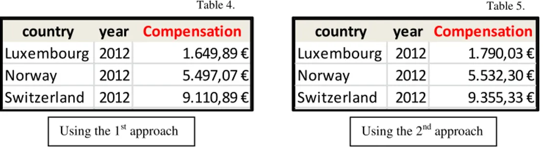
tables 4 and 5 are the amounts that would have to be given to an individual so that the
probabilities for the top 3 countries in 2012 are the same as in 2007, given that all other
variables are constant at 2012 values.
The values in the tables above are the required increases in the annual Income per capita
indicator for Portugal such that the probabilities of choice for each of the countries are
kept at 2007 values, given that all other variables are constant at 2012 values. There are
some interesting remarks regarding these values. Countries that had a larger increase in
the probability of choice from 2007 to 2012 show larger values for the respective
compensation, as are the cases of Norway and Switzerland, which show an increase of
their probabilities of 150% and 190%. For countries where the probability increase is
lower, the Compensation seems to be smaller. Luxembourg’s probability increases only
40%. Hence what seems to matter is the magnitude of the transition in the probability
and not the magnitude of the probability per se. What may shed light on these
statements is the fact that the model is inherently connected to a Random Utility
framework and that the subsequent behavior of the individual is the result of
maximization of utility and of responding in such way that is the best for him. This is
why there is a connection between the Compensating Variation and the adjustment of
16
See the annex for the conditions
country year Compensation
Luxembourg 2012 1.649,89 €
Norway 2012 5.497,07 €
Switzerland 2012 9.110,89 €
Denmark 2012 886,23 €
3.319,35 €
country year Compensation
Luxembourg 2012 1.790,03 €
Norway 2012 5.532,30 €
Switzerland 2012 9.355,33 € Australia 2012 16.093,86 €
825,06 € Using the 1st approach Using the 2nd approach
24
the probabilities via Income as done here. The probabilities of choice have an intrinsic
utility value. This model specification allows us to compute the Compensating
Variation using the choice probabilities and correcting for the transition in these choice
probabilities via the correct channel (de Palma, Killani, 2009). As a final note on this
analysis, I have used, for tables 6 and 7, the same process above to calculate the
adjustment via the Unemployment rate. Even though it is not a Compensation of any
kind I found that it was interesting to report.
These tables show us what adjustment to Portugal’s unemployment rate17
would be
required so that the probabilities of choice would remain in 2007 values, all else being
equal. Hence, the unemployment rate in Portugal should be 11% lower than it was to
keep the probability of choosing Luxembourg at 2007 values, all else being equal.
Again there seems to be the case that higher transitions in the probabilities of choice
imply higher adjustments.
17
For reference, the Unemployment Rate in Portugal was 15,6%.
country year Compensation
Luxembourg 2012 -11%
Norway 2012 -14%
Switzerland 2012 -14%
Using the 1st approach Using the 2nd approach
country year Compensation
Luxembourg 2012 -11%
Norway 2012 -14%
Switzerland 2012 -14%
25
5. CONCLUSION
This study focused on the migratory flows from Portugal to 31 Destination countries
during the years 2006 to 2012. To ascertain what causes were relevant to explain these
movements, I have used a Conditional Logit Model to calculate the Choice Probabilities
for each country in each year and to evaluate the significance of Income per capita,
Unemployment Rate, GDP growth factor and Distance in the individual’s decision
process. The first three factors are brought to the data in a ratio format since the most
likely and accurate way that an individual will absorb the information is by comparing
factors in Portugal and some Destination, and taking his decision based on compared
values instead of simple absolute values. The estimation strategy I used was segmented
in a linear, a fixed effects and a by year approach, in which Income per capita is
consistently significant cross approaches. Moreover I have calculated the Compensation
required to keep the probability of choice at 2007 values for the top 5 countries in 2012,
as a mean of reaching the value that would have to be given to an individual to present
choice probabilities equal to 2007, all else being equal. The fact that the model is rooted
in Discrete Choice Theory allows for this type of compensation to be computed, since it
derives from a Random Utility function maximization framework. Also, I have
employed the same exercise using the Unemployment Rate and calculated the value by
which this indicator would have to be adjusted in order to yield 2007 choice
26
REFERENCES
C. Simon Fan, Stark O., 2006. International migration and “educated unemployment”
Journal of Development Economics.
De Arce, Mahìa, 2008. Determinants of Bilateral Immigration flows between the
European Union and Mediterranean Partner Countries: Algeria, Egypt, Morocco,
Tunisia and Turkey. Munich Personas RePEc Archive paper nº14547
Greenwood M., Davies P., Li H., 2001. A Conditional Logit approach to U.S State to
State Migration. Journal of Regional Science, Vol. 41 nº2 , pp 337-360
Steins U., 2012. Determinants of Migration flows in Europe. Master thesis submitted in
2012, University of Bonn, under the supervision of Pf. F. Zimmermann.
Finnie R., 2004. Who moves ? A Logit model analysis of inter-provincial migration in
Canada. Applied Economics pp 1759-1779. Routledge. Taylor and Francis Group
Otrachshenko V., Popova O., 2013. Life (dis)satisfaction and the intention to migrate:
Evidence from Central and Eastern Europe. The Journal of Socio Economics 48 (2014)
pp 40- 49.
Stark O., 2005. Inequality and migration: A behavioral link. Institute of advanced
studies, Vienna, Austria. Economics Series nº 178.
De Palma A., Kilani K., 2009. Transition Choice in Probabilities and Welfare in
Additive Random Utility Models. Centre National de la Recherche Scientifique. Ecole
Polythechnique Department D’Economie.
Wooldridge J., 2005. Introductory Econometrics: A Modern Approach. Third Edition
Anderson, S.P., de Palma, A., Thisse, 1992. Discrete Choice Theory of
27
Annex
Figure 1. Descriptive Statistics of the Shares of Migrants of each country.
Figure 2. Correlation Matrix
Figure 3. All Choice probabilities for approach 1 and 2. Approach 3 is left out (can be reported on demand from the author) due to scale of the graph.
Incomepcratio Unemploymentratio Distance GDPgrowthratio
Incomepcratio 1 - -
-Unemploymentratio -0,477 1 -
-Distance 0,024 -0,354 1
-GDPgrowthratio 0,056 -0,202 0,027 1
0,00% 0,50% 1,00% 1,50% 2,00% 2,50% 3,00% 3,50% 4,00% 4,50% Au stra lia Au stri a Be lgi u m Can ad a Chi le Cze ch Rep De n m ar k Fi nl an d G erm an y H u n gary Ice lan d It al y Jap an Kore a La tv ia Li th u an ia Lu xe m b o u rg Me xi co N eth erl an d s N ew Z eal an d N o rw ay Po lan d Po rtu gal (No n -m o ve rs ) Ru ss ia Sl ov ak ia Sl ov en ia Sp ai n Sw ed en Sw itz erl an d Tu rk
ey UK USA
2006
30
Figure 4. Top 5 countries in terms of Choice Probabilities for the excluded years.
country year Inflow inc pc ratio unemp ratio distance gdp growth ratio1st approach
Luxembourg 2006 3,796 4,693827433 0,610389601 1.592,48 1,03437907 4,0420%
Norway 2006 0,097 3,804460953 0,441558465 2.780,25 1,008383465 1,7228%
Switzerland 2006 12,497 2,823136871 0,519480532 1.535,39 1,022703813 0,8401%
Iceland 2006 0,357 2,858254021 0,389610399 2.905,82 1,032141271 0,7201%
Denmark 2006 0,13 2,631335083 0,506493531 2.259,07 1,019186293 0,6401%
2nd approach
Luxembourg 2006 3,796 4,693827433 0,610389601 1.592,48 1,03437907 2,6301%
Norway 2006 0,097 3,804460953 0,441558465 2.780,25 1,008383465 1,5341%
Iceland 2006 0,357 2,858254021 0,389610399 2.905,82 1,032141271 0,7468%
Switzerland 2006 12,497 2,823136871 0,519480532 1.535,39 1,022703813 0,6972%
Denmark 2006 0,13 2,631335083 0,506493531 2.259,07 1,019186293 0,6119%
3rd approach
Luxembourg 2006 3,796 4,693827433 0,610389601 1.592,48 1,03437907 39,4567%
Norway 2006 0,097 3,804460953 0,441558465 2.780,25 1,008383465 15,8550%
Switzerland 2006 12,497 2,823136871 0,519480532 1.535,39 1,022703813 4,4287%
Germany 2006 4,917 1,837452192 1,337662396 1.952,78 1,022195605 3,7243%
Denmark 2006 0,13 2,631335083 0,506493531 2.259,07 1,019186293 3,4660%
country year Inflow inc pc ratio unemp ratio distance gdp growth ratio1st approach
Luxembourg 2008 4,531 4,695110221 0,671052627 1.592,48 0,992738632 4,2687%
Norway 2008 0,271 3,989402722 0,342105255 2.780,25 1,000760796 2,1381%
Switzerland 2008 17,772 2,873152351 0,447368439 1.535,39 1,021729431 0,9051%
Denmark 2008 0,136 2,623415836 0,447368439 2.259,07 0,992245842 0,6844%
Netherlands 2008 2,385 2,219175281 0,513157914 1.785,97 1,003506861 0,4942%
2nd approach
Luxembourg 2008 4,531 4,695110221 0,671052627 1.592,48 0,992738632 2,7513%
Norway 2008 0,271 3,989402722 0,342105255 2.780,25 1,000760796 1,8654%
Switzerland 2008 17,772 2,873152351 0,447368439 1.535,39 1,021729431 0,7489%
Denmark 2008 0,136 2,623415836 0,447368439 2.259,07 0,992245842 0,6545%
Iceland 2008 0,287 2,22243396 0,394736847 2.905,82 1,011966675 0,4811%
3rd approach
Luxembourg 2008 4,531 4,695110221 0,671052627 1.592,48 0,992738632 52,4066%
Norway 2008 0,271 3,989402722 0,342105255 2.780,25 1,000760796 11,9689%
Switzerland 2008 17,772 2,873152351 0,447368439 1.535,39 1,021729431 4,6506%
Spain 2008 16,857 1,453192365 1,486842149 346,17 1,009002754 3,6861%
Denmark 2008 0,136 2,623415836 0,447368439 2.259,07 0,992245842 2,5009%
country year Inflow inc pc ratio unemp ratio distance gdp growth ratio1st approach
Luxembourg 2009 3,844 4,481620576 0,536842095 1.592,48 0,972728417 3,8783%
Norway 2009 0,257 3,541600857 0,33684211 2.780,25 1,013116187 1,4146%
Switzerland 2009 13,67 2,969791176 0,431578937 1.535,39 1,010006286 1,0132%
Denmark 2009 0,152 2,538091361 0,631578947 2.259,07 0,971594279 0,6132%
Netherlands 2009 2,375 2,174590306 0,410526326 1.785,97 0,949571648 0,5476%
2nd approach
Luxembourg 2009 3,844 4,481620576 0,536842095 1.592,48 0,972728417 2,5827%
Norway 2009 0,257 3,541600857 0,33684211 2.780,25 1,013116187 1,3128%
Switzerland 2009 13,67 2,969791176 0,431578937 1.535,39 1,010006286 0,8269%
Denmark 2009 0,152 2,538091361 0,631578947 2.259,07 0,971594279 0,5855%
Netherlands 2009 2,375 2,174590306 0,410526326 1.785,97 0,949571648 0,5132%
3rd approach
Luxembourg 2009 3,844 4,481620576 0,536842095 1.592,48 0,972728417 55,0013%
Norway 2009 0,257 3,541600857 0,33684211 2.780,25 1,013116187 11,8137%
Switzerland 2009 13,67 2,969791176 0,431578937 1.535,39 1,010006286 6,5744%
Denmark 2009 0,152 2,538091361 0,631578947 2.259,07 0,971594279 3,7898%
31
Karush-Kuhn-Tucker Conditions for Local Optimality
Consider the following nonlinear optimization problem:
where x is the optimization variable, is the objective or cost function, are
the inequality constraint functions, and are the equality constraint
functions. The numbers of inequality and equality constraints are denoted m and l,
respectively.
country year Inflow inc pc ratio unemp ratio distance gdp growth ratio1st approach Luxembourg 2010 3,845 4,742012247 0,407407409 1.592,48 1,01142889 4,7732% Norway 2010 0,284 3,978918552 0,333333319 2.780,25 0,985694046 2,1867% Switzerland 2010 12,826 3,249896632 0,416666659 1.535,39 1,009974966 1,3027% Denmark 2010 0,168 2,607109039 0,694444432 2.259,07 0,994608888 0,6085% Netherlands 2010 1,958 2,16013258 0,361111114 1.785,97 1,000782987 0,5013% 2nd approach Luxembourg 2010 3,845 4,742012247 0,407407409 1.592,48 1,01142889 3,1091% Norway 2010 0,284 3,978918552 0,333333319 2.780,25 0,985694046 1,9071% Switzerland 2010 12,826 3,249896632 0,416666659 1.535,39 1,009974966 1,0250% Denmark 2010 0,168 2,607109039 0,694444432 2.259,07 0,994608888 0,5757% Australia 2010 0,226 2,393423314 0,481481455 16.203,29 1,001482947 0,5347% 3rd approach Luxembourg 2010 3,845 4,742012247 0,407407409 1.592,48 1,01142889 47,2875% Norway 2010 0,284 3,978918552 0,333333319 2.780,25 0,985694046 23,0753% Switzerland 2010 12,826 3,249896632 0,416666659 1.535,39 1,009974966 7,1416% Denmark 2010 0,168 2,607109039 0,694444432 2.259,07 0,994608888 3,6701% Iceland 2010 0,022 1,824557412 0,703703682 2.905,82 0,940794588 3,0990%
32
Necessary conditions for optimality:
Suppose that the objective function and the constraint
functions and are continuously differentiable at a point . If is
a local minimum that satisfies some regularity conditions then there exist
constants and , called KKT multipliers, such that
Stationarity
For maximizing f(x):
Primal feasibility
Dual feasibility
Complementary slackness
In the particular case , i.e., when there are no inequality constraints, the KKT
conditions turn into the Lagrange conditions, and the KKT multipliers are called Lagrange