Equatorial transport as diagnosed from nitrous oxide variability

(1)

ACPD

9, 4899–4930, 2009

Equatorial transport as diagnosed from

N₂O variability

P. Ricaud et al.

Title Page

Abstract Introduction

Conclusions References

Tables Figures

◭ ◮

Back Close

Full Screen / Esc

Printer-friendly Version

Interactive Discussion Atmos. Chem. Phys. Discuss., 9, 4899–4930, 2009

www.atmos-chem-phys-discuss.net/9/4899/2009/ © Author(s) 2009. This work is distributed under the Creative Commons Attribution 3.0 License.

Atmospheric Chemistry and Physics Discussions

This discussion paper is/has been under review for the journalAtmospheric Chemistry and Physics (ACP). Please refer to the corresponding final paper inACPif available.

Equatorial transport as diagnosed from

nitrous oxide variability

P. Ricaud1, J.-P. Pommereau2, J.-L. Atti é1,3, E. Le Flochmo ën1, L. El Amraoui3, H. Teyss èdre3, V.-H. Peuch3, W. Feng4, and M. P. Chipperfield4

1

Universit ´e de Toulouse, Laboratoire d’A ´erologie, CNRS UMR 5560, Toulouse, France

2

Service d’A ´eronomie, CNRS, Verri `eres-Le-Buisson, France

3

CNRM, M ´et ´eo-France, Toulouse, France

4

School of Earth and Environment, University of Leeds, Leeds, UK

Received: 11 December 2008 – Accepted: 2 February 2009 – Published: 24 February 2009

Correspondence to: P. Ricaud (philippe.ricaud@aero.obs-mip.fr)

(2)

ACPD

9, 4899–4930, 2009

P. Ricaud et al.

Title Page

Tables Figures

◭ ◮

Back Close

Full Screen / Esc

Interactive Discussion

Abstract

The mechanisms of transport on annual, semi-annual and quasi-biennial time scales in the equatorial (10◦S–10◦N) stratosphere are investigated using the nitrous oxide (N2O) measurements of the space-borne ODIN Sub-Millimetre Radiometer instrument from November 2001 to June 2005, and the simulations of the three-dimensional Chemistry 5

Transport Models MOCAGE and SLIMCAT. Both models are forced with analyses from the European Centre for Medium-range Weather Forecasts, but the vertical transport is derived either from the forcing analyses by solving the continuity equation (MOCAGE), or from diabatic heating rates using a radiation scheme (SLIMCAT). The N2O variations in the mid-to-upper stratosphere at levels above 32 hPa are shown to be generally 10

captured by the models though significant differences appear with the observations as well as between the models, attributed to the difficulty of capturing correctly the slow vertical velocities of the Brewer-Dobson circulation. In the lower stratosphere (LS), below 32 hPa, the variations are shown to be principally seasonal with peak amplitude at 400 K (∼19 km), and are totally missed by the models. The decrease in diabatic 15

radiative heating in the LS during the Northern Hemisphere summer is found to be out of phase by one month and far too small to explain the observed N₂O seasonal cycle. The proposed explanation for this annual variation is a combination of i) the annual cycle of tropopause height of 1 km amplitude, ii) the convective overshooting above 400 K peaking in May and absent in the models, and iii) an annual cycle of 15 ppbv 20

amplitude of the N2O concentration at the tropopause, but for which no confirmation exists in the upper troposphere in the absence of global-scale measurements. The present study indicates i) a significant contribution of deep convective overshooting on the chemical composition of the LS at global scale up to 500 K, ii) a preferred region for that over the African continent, and iii) a maximum impact in May when the overshoot 25

(3)

ACPD

9, 4899–4930, 2009

P. Ricaud et al.

Title Page

Tables Figures

◭ ◮

Back Close

Full Screen / Esc

1 Introduction

Nitrous oxide (N2O) is an excellent tracer of atmospheric vertical transport since its sources are located in the troposphere (soils, wetlands, biomass burning and industrial emissions) where its lifetime is around 100 years. Its sink is in the stratosphere essen-tially by photolysis and reaction with electronically-excited oxygen atoms O(1D), the 5

primary source of stratospheric odd nitrogen (NOy) (e.g. Brasseur et al., 1999), where its lifetime is less than one year. It is also a greenhouse gas and contributes to climate change (IPCC, 2001). After entering the stratosphere at the tropical tropopause, N2O, like all long-lived species, is transported by the Brewer-Dobson circulation to high al-titudes and then to the polar regions. Its spatial and temporal distribution can be thus 10

used as a straightforward diagnostic of global-scale transport processes at different timescales, from seasons to decades.

In the mid and upper stratosphere, due to its long lifetime, the equatorial N₂O fields exhibit a strong semi-annual oscillation (SAO), as shown by Randel et al. (1994) from two years of Cryogenic Limb Array Etalon Spectrometer (CLAES) observations. This 15

behaviour was recently confirmed by Jin et al. (2008) from the measurements of the Microwave Limb Sounder (MLS) on the AURA platform, the Atmospheric Chemistry Experiment Fourier Transform Spectrometer (ACE-FTS) and the Sub-Millimetre Ra-diometer (SMR) aboard ODIN. Furthermore, combining N₂O from CLAES in 1991– 1993 (O’Sullivan and Dunkerton, 1997), CH4, and H2O from the Halogen Occultation 20

Experiment (HALOE) on the Upper Atmosphere Research Satellite (UARS) and O3 from the Stratospheric Aerosol and Gas Experiment II (SAGE II) on the Earth Radi-ation Budget Experiment (ERBE), Randel and Wu (1996) and Baldwin et al. (2001) demonstrated the influence of the quasi-biennial oscillation (QBO) on the distribution of long-lived species in the equatorial belt.

25

(4)

ACPD

9, 4899–4930, 2009

P. Ricaud et al.

Title Page

Tables Figures

◭ ◮

Back Close

Full Screen / Esc

Interactive Discussion of the annual oscillation (AO) and the QBO (Randel et al., 2007; Schoeberl et al., 2008),

whilst Gettelman et al. (2004) explored the impact of the monsoon during the June– August period. Finally, Ricaud et al. (2007) from a combination of ODIN N2O, HALOE CH₄and MLS CO observations have shown the large variations of species concentra-tions in the equatorial low stratosphere in March–April–May (MAM), displaying marked 5

maxima over Africa and other land areas, very consistent with the overshooting picture derived from the Tropical Rainfall Measuring Mission (TRMM) Precipitation Radar.

As an extension of the previous study, here we investigate how N2O behaves in the entire equatorial stratosphere including the Tropical Tropopause Layer (TTL) over a five year time period by combining ODIN/SMR measurements from 2001 to 2006 10

and long-term runs of the three-dimensional (3-D) chemical transport models (CTMs) SLIMCAT and MOCAGE. Particular attention will be paid to the UTLS to see how the contrast between land and oceanic regions observed by Ricaud et al. (2007) in MAM 2002–2004, extends to other seasons.

Information on the ODIN N2O observations and model simulations are provided in 15

Sect. 2. Section 3 is devoted to the presentation of the time evolution of N2O in the stratosphere from November 2001 to June 2005 in the equatorial belt and the influence of annual, semi-annual and quasi-biennial oscillations. Section 4 concentrates on the annual oscillation in the lower stratosphere and its possible explanations. Section 5 summarises our findings.

20

2 Observations and models

2.1 ODIN

The data used here are from the ODIN/SMR instrument. The ODIN mini-satellite (Murtagh et al., 2002) was placed into a 600-km sun-synchronous, terminator orbit in February 2001 and is still operational. The platform includes the SMR microwave 25

(5)

ACPD

9, 4899–4930, 2009

P. Ricaud et al.

Title Page

Tables Figures

◭ ◮

Back Close

Full Screen / Esc

Interactive Discussion the frequency domain 480–580 GHz, most of its measurements being validated (e.g.

Barret et al., 2006). The present study is based on the retrievals of the 502.296-GHz N2O line using the Optimal Estimation Method (Rodgers, 2000). On average, N2O measurements are performed one day out of three, due to sharing of the instrument with astronomy. All measurements performed between November 2001 and July 2005 5

have been analyzed using version V222 of the retrieval algorithm (Urban et al., 2005). Note that from November 2005 to October 2006, ODIN N₂O data has been processed using version V225 of the retrieval algorithm but this data is not used in the present analysis that only covers November 2001–June 2005. The vertical resolution is 2 km. The single-scan precision ranges from 10 to 45 ppbv for N₂O mixing ratios varying from 10

0 to 325 ppbv. The total systematic error varies from 3 to 35 ppbv for N₂O mixing ra-tios from 0 to>_{150 ppbv. In the UTLS, the single scan precision is}_∼_{39 and}_∼_{24 ppbv}

(∼10–12%) at 100 hPa and 70 hPa, respectively and the total systematic error is ∼22 and∼13 ppbv (∼4–6%), respectively. All measurements have been averaged into bins of 10◦latitude×30◦longitude.

15

2.2 SLIMCAT

SLIMCAT is an off-line 3-D CTM described in detail in Chipperfield (1999). The model uses a hybridσ₋θvertical coordinate and extends from the surface to a top level which depends on the domain of the forcing analyses. Vertical advection in the θ_-level

do-main (above 350 K) is calculated from diabatic heating rates using a radiation scheme 20

which gives a better representation of vertical transport and age-of-air even with Eu-ropean Centre for Medium-range Weather Forecasts (ECMWF) ERA40 analyses than using vertical winds derived from the analyses which have known problems (Chip-perfield, 2006). The model contains a detailed stratospheric chemistry scheme. The present experimental set up is detailed in Feng et al. (2007). The horizontal resolution 25

is 7.₅◦_×₇.₅◦ _{with 24 levels from the surface to about 60 km. The model was forced}

(6)

ACPD

9, 4899–4930, 2009

P. Ricaud et al.

Title Page

Tables Figures

◭ ◮

Back Close

Full Screen / Esc

Interactive Discussion et al., 2005), and after this date, the operational analyses are employed. In the run

used here there is no explicit treatment of tropospheric convection. The troposphere is assumed well mixed, i.e. tropospheric trace gases are mixed with a contant volume mixing ratio profile up to the tropopause (380 K in the tropics). The time evolution of surface mixing ratios of greenhouse gases (particularly N₂O) is prescribed according 5

to the Intergovernmental Panel on Climate Change (IPCC) recommendations (IPCC, 2001). Furthermore, the model run covers the period 1977–2005 for studying the long-term evolution of N₂O but only equatorial (10◦_S–10◦_{N) zonally-averaged N}

2O data from November 2001 to June 2005 are used in the present study.

2.3 MOCAGE 10

MOCAGE-Climat (Teyss èdre et al., 2007) is the climate version of M ét éo-France’s tropospheric-stratospheric MOCAGE 3-D CTM. The climate version used in this study has 60 layers from the surface up to 0.07 hPa, with a horizontal resolution of 5.₆◦_×₅.₆◦_.

ECMWF 6-hourly analyses were used to force the model from 1 January 2000 to 31 December 2005. MOCAGE uses a semi-Lagrangian advection scheme and vertical 15

velocities are recalculated from the forcing analyses by solving continuity equation. MOCAGE-Climat contains a detailed tropospheric-stratospheric chemistry scheme. Initial chemical conditions were taken from a previous simulation to allow the model to quickly reach its numerical equilibrium, especially for long-lived species, such as N2O. Surface emissions prescribed in MOCAGE-Climat are based upon yearly- or monthly-20

averaged climatology. The N₂O surface emissions are taken from the Global Emissions Inventory Activity and are climatology representative of the year 1990 (Bouwman et al., 1995). They include anthropogenic and biogenic sources, for a total emission rate of 14.7 Tg(N) yr−1_{. Note that, regarding convection, the present run was performed using} the scheme of Betchold et al. (2001). Modelled data have been averaged into bins of 25

(7)

ACPD

9, 4899–4930, 2009

P. Ricaud et al.

Title Page

Tables Figures

◭ ◮

Back Close

Full Screen / Esc

3 Influence of transport on the N₂O stratospheric distribution

The N2O anomaly (defined as the difference between the N2O field and its mean and linear trend over the period) in the ODIN, MOCAGE and SLIMCAT data sets during the period 2000–2006 from 100 to 1 hPa is shown in Fig. 1, onto which the ECMWF zonal wind u _{is superimposed. Easterlies (westerlies) are represented by solid (dashed)}

5

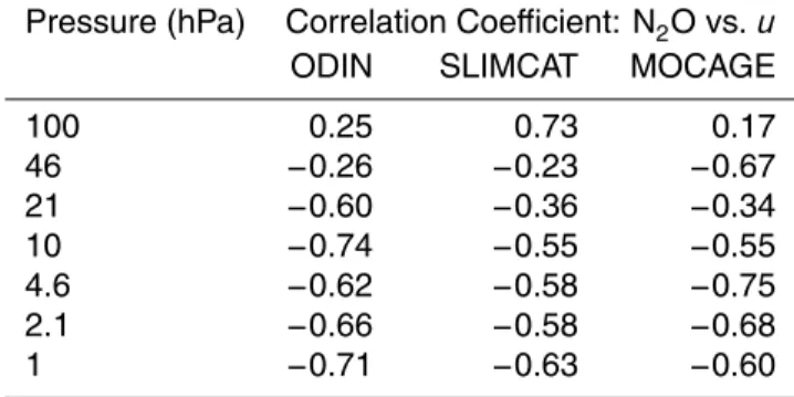
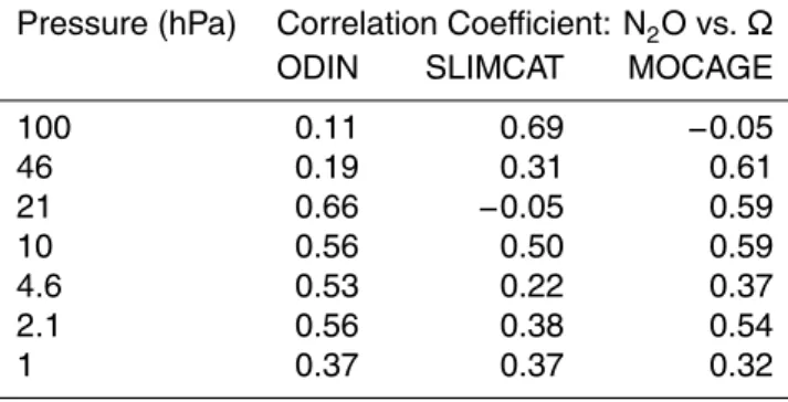
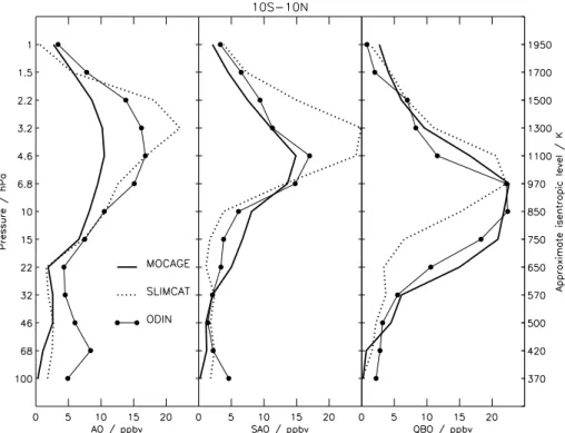
lines. The vertical distributions of the amplitude of the AO, SAO and QBO during the November 2001–June 2005 overlapping period derived from these data are shown in Fig. 2 as a function of pressure. The correlation coefficients between N2O concen-trations and ECMWF zonal and vertical winds calculated from the integration of the mass-conservative continuity equation are displayed in Tables 1 and 2, respectively. 10

3.1 Mid-to-upper stratosphere (32–1 hPa)

In the mid-to-upper stratosphere, the three oscillations (AO, SAO and QBO) compete in the ODIN observations, the AO and SAO dominating in the upper stratosphere (5–1 hPa) and the QBO in the middle stratosphere (32–5 hPa). A strong AO signal is seen from 22 to 1 hPa with a broad maximum at around 4.6 hPa of ∼15 ppbv. As 15

shown by Schoeberl et al. (2008), the AO signal results from the annual variation of the vertical velocity in the lower stratosphere. The correlationr between N₂O and vertical winds is moderately high, i.e. 0.53–0.66 between 21–2.1 hPa.

A strong SAO signal is observed in the upper stratosphere with marked positive anomalies occurring every two years in 2002, 2004 and 2006. As already noted by 20

Schoeberl et al. (2008) and Jin et al. (2008), the positive (negative) anomalies in the upper stratosphere SAO cycle are in phase with westerly (easterly) QBO phases in the middle stratosphere. The SAO contribution is significant from 10 to 1.5 hPa with a maximum of about 15 ppbv at 4.6 hPa.

A QBO signal also appears in the middle stratosphere with a downward propagation 25

(8)

damp-ACPD

9, 4899–4930, 2009

P. Ricaud et al.

Title Page

Tables Figures

◭ ◮

Back Close

Full Screen / Esc

Interactive Discussion ing in the stratosphere of several waves (Rossby, Kelvin, gravity waves, etc.), excited

by diabatic thermal process in the troposphere (e.g. Cariolle et al., 1993). The QBO easterly (westerly) phase at 40 hPa is associated with an upward (downward) mean meridional circulation bringing N2O-rich (-poor) air upward (downward). Since east-erlies are stronger and last longer than westeast-erlies, the positive N₂O anomaly in the 5

data also lasts longer than the negative anomaly with a downward propagation from 4.6 to 21 hPa consistent with model calculations of 1 km month−1. Around 20–30 hPa and below, the westerly wind regime propagates downward at constant velocity with little variation between cycles, whilst the descent speed of easterlies slows down at lower altitude (Kinnersley and Pawson, 1996). Because of the stalling of easterlies, the 10

time between maximum easterlies and maximum westerlies is much shorter than the reverse (Naujokat, 1986). This explains the asymmetric descent rates of easterly and westerly regimes seen in the N2O concentration with positive anomalies lasting longer than negative ones in the lower stratosphere. The QBO signal extends from 32 to 1 hPa with a maximum amplitude of∼20 ppbv peaking at 10 hPa. The anti-correlationr 15

between N2O data and zonal winds is indeed very high (0.60–0.74) between 21 and 1 hPa.

The two CTMs globally match the data above 32 hPa to within±5 ppbv as well as the amplitude of the AO, SAO and QBO signals (Fig. 2), in contrast to the CMAM chemistry-climate model (Jin et al., 2008), which cannot capture the QBO structure. Nevertheless, 20

some significant differences with the observations are also apparent. The SLIMCAT AO signal is consistent with that of ODIN, but MOCAGE underestimates its amplitude by 5–10 ppbv between 2.2 and 6.8 hPa. The SLIMCAT SAO is 10–15 ppbv larger than that observed between 2.2 and 4.6 hPa, which is better matched by MOCAGE. Finally, the QBO is very well reproduced by MOCAGE, whereas SLIMCAT underestimates its 25

amplitude by 10–15 ppbv between 10 and 20 hPa.

(9)

ACPD

9, 4899–4930, 2009

P. Ricaud et al.

Title Page

Tables Figures

◭ ◮

Back Close

Full Screen / Esc

Interactive Discussion SLIMCAT and 5.₆◦

×5.6◦ for MOCAGE) may contribute, the major difference likely re-sults in their method for calculating the vertical advection, forced by ECMWF analyses in MOCAGE and derived from diabatic heating rates in SLIMCAT. The anti-correlation between N₂O and zonal winds (Table 1) is indeed very high (0.55–0.75) in MOCAGE and SLIMCAT between 10 and 1 hPa, as observed. However, the correlation between 5

N2O and vertical winds (Table 2) between 2.1 and 10 hPa is rather poor in SLIMCAT (0.22–0.50) whilst in MOCAGE the correlation is greater (0.37–0.59) and somewhat more consistent, although smaller, with the ODIN values (0.53–0.56). Once again, this illustrates the importance of vertical advection in the control of the vertical distribution of chemical species in the stratosphere, but also the difficulty of reproducing these 10

small vertical velocities in models.

3.2 UTLS (100–32 hPa)

At altitudes below 32 hPa, the AO dominates in the observations, except at 100 hPa where a SAO signal of similar magnitude can be seen. Compared to this, the AO is almost missing in the models, while both the SAO and the QBO are underestimated in 15

the TTL at levels below 68 hPa. In contrast with the models displaying correlation be-tween N₂O concentration and ECMWF vertical advection (0.69 in SLIMCAT at 100 hPa, and 0.61 in MOCAGE at 46 hPa), the observed variations are totally disconnected from these. The inability of the models to reproduce observations suggests that other mech-anisms, not currently included or poorly treated in the model schemes, are controlling 20

the N2O cycle at these levels.

4 Annual oscillation in the UTLS

(10)

ACPD

9, 4899–4930, 2009

P. Ricaud et al.

Title Page

Tables Figures

◭ ◮

Back Close

Full Screen / Esc

Interactive Discussion modelled monthly mean N₂O concentration at 100, 68, 46 and 32 hPa, the levels of

the ODIN/SMR measurements, averaged between November 2001 and June 2005. To identify possible geographic differences in the observations reported by Ricaud et al. (2007), also shown are the mean concentrations over the African (30◦W–60◦E) and the Western Pacific (120◦E–150◦W) sectors. To subtract the contribution of the 5

well-known seasonal cycle of isentropic surface height on which the mixing ratio would remain constant if no diabatic vertical transport was involved, the N₂O fields have been linearly interpolated on potential temperature surfaces. Figure 4 shows the seasonal variations of N2O fields interpolated at 400, 450, 500 and 550 K and Fig. 5 displays the contrast between African and Western Pacific sectors. Figure 6 shows the seasonal 10

cycles of NCEP tropopause temperature and pressure, upwelling from thermodynamic balance from Randel et al. (2007), and potential temperature changes between 15– 23 km. A minimum height and maximum temperature of the tropopause, and a max-imum potential temperature at levels above peaking at 19 km is observed in August, while the minimum upwelling occurs one month earlier.

15

4.1 Seasonal cycle

A seasonal cycle is observed in the ODIN zonal mean (black dots) at all levels with a minimum from May to August at 100 hPa (∼16.5 km) or 400 K (∼18 km), extending to September at higher altitude. Its amplitude is a maximum at 68 hPa and 400 K. The minimum N2O in June is consistent with that derived by Jin et al. (2008) from 20

the same ODIN observations (using the Swedish algorithm version 2.1 from July 2001 to February 2007), as well as from AURA/MLS, although the broader MLS vertical resolution results in a weaker contrast. A small semi-annual oscillation (secondary minimum in January) can also be seen at 100 hPa in Fig. 3, but disappears in the potential temperature plots in Fig. 4, suggesting an influence of the tropopause height. 25

(11)

mean-ACPD

9, 4899–4930, 2009

P. Ricaud et al.

Title Page

Tables Figures

◭ ◮

Back Close

Full Screen / Esc

Interactive Discussion ing that the minimum propagates upward far faster than the 0.2–0.3 km month−1of the

Brewer-Dobson circulation (Mote et al., 1996). The absence of N2O phase shift with altitude in the lower stratosphere was also noticed by Schoeberl et al. (2008) in the MLS data, and was attributed to the signature to the seasonal variation of the Brewer-Dobson upward velocity. However, since the minimum N2O is observed in June, one 5

month in advance relative to the minimum upward velocity in July (Randel et al., 2007 and Fig. 6), there is a contradiction which is difficult to reconcile.

However, most important for understanding the mechanism responsible for the AO is the contrast between the Western Pacific and the African sectors being maximum in May–July at 100 hPa (16.5 km) and at 400 K (18 km), and insignificant above, except in 10

May (Fig. 5). The amplitude of the seasonal cycle is smaller above Africa than above the Western Pacific at 100 hPa and at 400 K.

Compared to the observations, the two models show little seasonal variation. SLIM-CAT displays a slight minimum in August–September of small amplitude consistent with the known minimum diabatic radiative heating in July–August (e.g. Randel et al., 2007 15

and Fig. 6), shifted by 1 month because of the slow ascent rate of 600–800 m month−1. Given the assumed well mixed troposphere in SLIMCAT, this annual cycle reflects the varying altitude of the model tropopause. MOCAGE also shows almost no seasonal variation but the well-known ECMWF too fast ascent of the Brewer-Dobson circulation above 21 km (Monge-Sanz et al., 2007, and references therein). The same applies 20

to the CMAM model which underestimates the amplitude of the minimum N₂O shifted also to August–September (Jin et al., 2008). In summary, the N2O seasonal cycle in the TTL and lower stratosphere reported by ODIN requires mechanisms which do not exist in the currently available CTM global models.

4.2 Discussion 25

(12)

ACPD

9, 4899–4930, 2009

P. Ricaud et al.

Title Page

Tables Figures

◭ ◮

Back Close

Full Screen / Esc

Interactive Discussion 4.2.1 Possible contributions

Ignoring here the specific issue of water vapour which involves still unresolved ques-tions of hydration-dehydration processes, the presence of a seasonal cycle in the con-centration of several tropospheric tracers, as well as ozone, in the tropical UTLS has been already noted by Folkins et al. (2006), Randel et al. (2007), Jin et al. (2008), and 5

Schoeberl et al. (2008). The AO is generally attributed to the seasonal cycle of the vertical velocity of the diabatic heating and the Brewer-Dobson circulation. However, there are differences in the phase of the AO between the species difficult to reconcile with a minimum vertical velocity in July. An ozone maximum and a carbon monoxide minimum are observed in August (Randel et al., 2007) peaking at about 17.5 km and 10

100 hPa, respectively and, from the present study, a minimum N2O occurs in June at 18–19 km propagating to 21–22 km with no phase shift, one-month ahead the minimum in upwelling in July.

Several mechanisms could contribute to the AO whose impacts will depend on the lifetime and on the vertical distribution of the species. The first is the vertical transport of 15

the species by diabatic heating or height displacement of the tropopause and isentropic surfaces immediately above, both displaying a seasonal cycle but shifted by one month (Fig. 6). The amplitude of the variation of concentration of the species at a given altitude or pressure level will depend on its vertical gradient at this level. It will be large for ozone for which a vertical displacement of only 250 m within a vertical gradient of 20

0.8 ppmv km−1 could explain the 0.15 ppmv amplitude of the AO at 17.5 km seen by Randel et al. (2007). It will be smaller for CO for which the same displacement within a vertical gradient of−14 ppbv km−1will result in a change of 3.5 ppbv only at 17.5 km. It will be very small for N2O since a vertical gradient of−6 ppbv km−

1

will only produce a 1.5 ppbv change in the lower stratosphere.

25

(13)

ACPD

9, 4899–4930, 2009

P. Ricaud et al.

Title Page

Tables Figures

◭ ◮

Back Close

Full Screen / Esc

Interactive Discussion within one year is negligible.

The third contributing parameter is the seasonal cycle of the species in the upper troposphere (UT) resulting from variations of surface source emissions, chemical pro-cesses (e.g. lightning NOx) and convective lifting. In the case ozone, the seasonal change in the tropical UT is limited to 30–40 ppbv maximum at 15 km (Randel et al. 5

2007). The CO variation at 147 hPa shows a small (5 ppbv) AO but a larger SAO of 25 ppbv amplitude with minima in December–February and July–September (Randel et al., 2007). Unfortunately there is little information on N₂O in the UT, only recent in-dications from the nadir-viewing Infrared Atmospheric Sounding Interferometer (IASI) aboard MetOp-A of a maximum total column (mainly in the mid-troposphere) in the 10

equatorial belt in MAM 2008 over Africa (Ricaud et al., 2008).

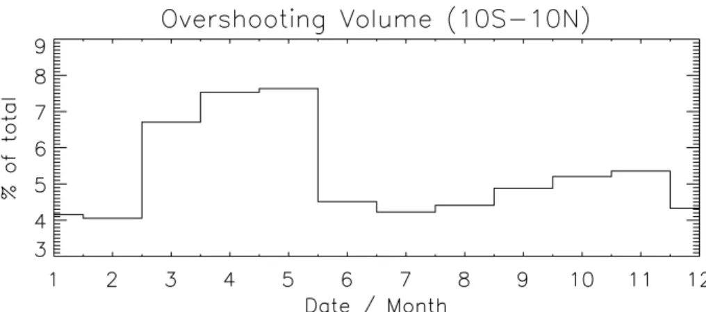
The fourth and last potential contributor to an AO cycle is the fast convective over-shooting of tropospheric air above continental regions and particularly Africa, between February and May and, to a lesser extent, in September–November as shown by the overshooting volume in the 10◦S–10◦N band (Fig. 7) derived from the TRMM precip-15

itation radar overshooting features (Liu and Zipser, 2005). This mechanism was that suggested by Ricaud et al. (2007) for explaining the contrast in N₂O, CH₄ and CO concentrations in the lower stratosphere between the Western Pacific, Africa and other continental areas. However, the amplitude of the contrast between various regions will also depend on the zonal wind velocity that is the time needed for local injections in 20

preferred regions to mix up at zonal scale. The seasonal cycle of each species will be a combination of all these parameters whose impacts will depend on the specific characteristics of each species.

4.2.2 Ozone

Because of its maximum vertical gradient at 17.5 km, the ozone AO (Randel et al., 25

(14)

ACPD

9, 4899–4930, 2009

P. Ricaud et al.

Title Page

Tables Figures

◭ ◮

Back Close

Full Screen / Esc

Interactive Discussion stations during the period of minimum ozone in February–March. A vertical

displace-ment of 250 m in the 0.8 ppmv km−1

vertical gradient will be enough to explain the 0.15 ppmv amplitude of the cycle. The very limited AO amplitude at 20 km suggests that the main process responsible could be the seasonal variation of isentropic surface heights of rapidly decreasing amplitude with altitude above the tropopause.

5

From Fig. 6, if we consider the two time distributions of the tropopause pressure and of the upwelling, although both of them are peaking in July, the minimum of the distribution is located end of July for the upwelling and mid of August for the tropopause pressure. The ozone and tropopause pressure cycles are thus perfectly in phase, in contrast with the one-month shift of the ascent by radiative heating which would require 10

only 10 days for a 250 m displacement.

4.2.3 Carbon monoxide

The CO seasonal cycle at 68 hPa (19 km) (Randel et al., 2007) shows a minimum in September–November shifted by 2–3 months compared to the radiative ascent rate, followed by a fast increase in November–December and a maximum in February– 15

March. Since a vertical displacement, either radiative ascent or isentropic surface lift, will have a limited impact on the concentration of the species, the observations will be better compatible with overshooting during the convective season in February–May, followed by a 40% photochemical reduction during the following 5 months. Overshoot episodes, such as those reported by Ricaud et al. (2007), could also explain the fast 20

(15)

ACPD

9, 4899–4930, 2009

P. Ricaud et al.

Title Page

Tables Figures

◭ ◮

Back Close

Full Screen / Esc

Interactive Discussion 4.2.4 Nitrous oxide

N2O (Fig. 3) displays a zonal mean seasonal cycle of 15 ppbv amplitude at 100 hPa, increasing to 20 ppbv at 68 hPa (19 km), and then reducing progressively at higher al-titude, with a minimum in May–July. Within an average−6 ppbv km−1vertical gradient as observed by ODIN at least above 68 hPa, this would correspond to a vertical dis-5

placement of 2.5, 3.3, 2.0 and 1.7 km at 100, 68, 46 and 32 hPa, respectively. After interpolation on isentropic surfaces for correcting for the seasonal variation of the isen-tropic surface height (Fig. 4), the amplitude is slightly reduced by 1–3 ppbv. The main consequence is the reduction of the September–October maximum at 400 K and that of November–December at 450 K and thus the removal of the SAO signal. However, 10

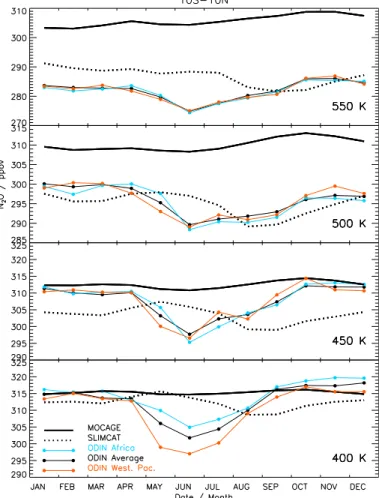
most apparent is the larger amplitude of the cycle above the Western Pacific (19 ppbv) than over Africa (14 ppbv) at 400 K (Fig. 5), the contrast being maximum (12 ppbv) in May. Except in May, this contrast vanishes at higher altitude.

Since the minimum N2O occurs one month before the drop in the upwelling calcu-lated from thermodynamic balance (Randel et al., 2007) and since its amplitude would 15

imply a relative subsidence of−1.1 mm s−1(−1.9 K day−1) in contradiction with all cal-culations (Folkins et al., 2006; Corti et al., 2005), the N2O seasonal cycle cannot be explained by the modulation of the vertical transport by radiative heating. Instead, the peak contrast between the Western Pacific and Africa in May up to 500 K (21 km) coincident with that of the maximum overshooting volume derived from the TRMM ob-20

servations, suggests a clear contribution of deep convective overshooting combined with a small horizontal mixing during the period of minimum zonal wind (Fig. 8).

However, this process alone should result in an increase of the N₂O concentration and not the opposite; something else is required. Figure 9 shows the seasonal change of the ODIN N2O vertical profile as well as those of the models. The strong gradi-25

(16)

ACPD

9, 4899–4930, 2009

P. Ricaud et al.

Title Page

Tables Figures

◭ ◮

Back Close

Full Screen / Esc

Interactive Discussion those changes, MOCAGE showing too fast vertical transport almost constant

through-out the year and SLIMCAT, based on radiative calculations, slower average velocity with a slight minimum in August–September.

However, the picture also shows that the May–August minimum concentration origi-nates at the bottom of the profile, at the tropopause, implying a large seasonal change 5

in the UT. Unfortunately, apart from the recent IASI total columns consistent with the ODIN indications at 100 hPa (Ricaud et al., 2008), there is no N₂O measurement avail-able in the UT to confirm unambiguously the hypothesis. MOCAGE (Fig. 10) displays a maximum in NDJ associated to convective activity over Africa, consistent with ODIN, but of only 1.5 ppbv amplitude instead of the observed 15 ppbv. However, since sea-10

sonal changes in the surface sources and overshooting are ignored in the model, this is of limited significance.

In summary, the observed ODIN N2O seasonal cycle in the lower stratosphere, dif-ferent to those of O₃ and CO, and the contrast of concentration between the Western Pacific and the African sectors, would be the result of a minimum N2O concentration in 15

the upper troposphere in May–July and deep convective overshooting in February–May combined with a minimum horizontal mixing in May–June.

The above findings fully confirm the hypothesis of the convective origin of the larger N2O concentration over Africa than over the Western Pacific during the March–May period reported earlier by Ricaud et al. (2007) and thus the significant contribution 20

of convective overshooting on the chemical composition of the lower stratosphere at global scale up to 20–21 km altitude.

5 Conclusions

The evolution of the concentration of the long-lived N2O species in the stratosphere has been studied from the measurements of the space-borne ODIN/SMR instrument 25

(17)

ACPD

9, 4899–4930, 2009

P. Ricaud et al.

Title Page

Tables Figures

◭ ◮

Back Close

Full Screen / Esc

Interactive Discussion two chemistry transport models (CTMs), both forced with ECMWF analyses, whilst the

vertical transport is derived from the forcing analyses by solving the continuity equation (MOCAGE) and from diabatic heating rates using a radiation scheme (SLIMCAT).

The observed N₂O variations are found to be influenced by the annual, semi-annual and quasi-biennial oscillations of comparable amplitudes in the mid-stratosphere, whilst 5

the AO dominates below 32 hPa with amplitude peaking at 68 hPa, and a significant SAO signature at 100 hPa. Both CTMs generally match the data above 32 hPa to within±5 ppbv as well as the amplitude of the AO, SAO and QBO signals. However, significant differences appear with the observations as well as between the models, attributed to the difficulty of capturing correctly the slow vertical velocities of the Brewer-10

Dobson circulation.

The situation is worse in the lower stratosphere where the models, although one of them includes radiative heating, totally miss the annual oscillation. The drop of diabatic radiative heating during the Northern Hemisphere summer in July is found to be out of phase by one month and far too small for explaining the observations. The processes 15

involved are shown to be a combination of the annual variation of tropopause height of 1 km amplitude, convective overshooting up to 500 K totally ignored in the models, and an annual cycle of 15 ppbv amplitude of the N2O concentration observed at the tropopause, but for which there is still little confirmation in the upper troposphere in the absence of global-scale profile measurements. The larger N₂O concentration in the 20

lower stratosphere over Africa compared to the Western Pacific during the convective period reported by Ricaud et al. (2007) is fully confirmed. The most important impli-cation of the findings is the demonstration of the significant contribution of convective overshooting on the chemical composition of the lower stratosphere at the global scale up to 500 K (20–21 km).

25

(18)

ACPD

9, 4899–4930, 2009

P. Ricaud et al.

Title Page

Tables Figures

◭ ◮

Back Close

Full Screen / Esc

Interactive Discussion NCEO.

The publication of this article is financed by CNRS-INSU.

References

5

Baldwin, M. P., Gray, L. J., Dunkerton, T. J., et al.: The quasi-biennial oscillation, Rev. Geophys., 39, 179–229, 2001.

Barret, B., Ricaud, P., Santee, M. L., et al.: Intercomparisons of trace gases profiles

from the Odin/SMR and Aura/MLS limb sounders, J. Geophys. Res., 111, D21302, doi:10.1029/2006JD007305, 2006.

10

Betchold, P., Bazile, E., Guichard, F., et al.: A mass flux convection scheme for regional and global models, Q. J. Roy. Meteor. Soc., 127, 869–886, 2001.

Bouwman, A. F., Van der Hoek, K. W., and Olivier, J. G. J.: Uncertainties in the global source distribution of nitrous oxide, J. Geophys. Res., 100(D2), 2785–2800, 1995.

Brasseur, G., P., Orlando, J. J., and Tyndall, G. S.: Atmospheric Chemistry and Global Change, 15

2nd edn., Oxford University Press, New York, Oxford, ISBN-0-19-510521-4, 1999.

Cariolle, D., Amodei, M., D ´equ ´e, M., et al.: A quasi-biennal oscillation signal in general circula-tion model simulacircula-tions, Science, 261, 1313–1316, 1993.

Chipperfield, M. P.: Multiannual simulations with a three-dimensional chemical transport model, J. Geophys. Res., 104, 1781–1805, 1999.

20

Chipperfield, M. P.: New version of the TOMCAT/SLIMCAT offline chemical transport model:

intercomparison of stratospheric tracer experiments, Q. J. Roy. Meteor. Soc., 132, 1179– 1203, doi:10.1256/qj.05.51, 2006.

(19)

ACPD

9, 4899–4930, 2009

P. Ricaud et al.

Title Page

Tables Figures

◭ ◮

Back Close

Full Screen / Esc

Interactive Discussion mass fluxes in the equatorial upper troposphere and lower stratosphere, Geophys. Res. Lett.,

32, L06802, doi:10.1029/2004GL021889, 2005.

Feng, W., Chipperfield, M. P., Dorf, M., et al.: Mid-latitude ozone changes: studies with a 3-D CTM forced by ERA-40 analyses, Atmos. Chem. Phys., 7, 2357–2369, 2007,

http://www.atmos-chem-phys.net/7/2357/2007/. 5

Folkins, I., Bernath, P., Boone, C., Lesins, G., Livesey, N., Thompson, A. M., Walker, K., and Witte, J. C.: Seasonal cycles of O₃, CO and convective outflow at the tropical tropopause, Geophys. Res. Lett., 33, L16802, doi:10.1029/2006GL026602, 2006.

Frisk, U., Hagstr ¨om, M., Ala-Laurinaho, J., et al.: The Odin satellite I: Radiometer design and test, Astron. Astrophys., 402, L27–L34, doi:10.1051/0004 6361:20030335, 2003.

10

Gettelman, A., Kinnison, D. E., Dunkerton, T. J., and Brasseur, G. P.: Impact of monsoon cir-culations on the upper troposphere and lower stratosphere, J. Geophys. Res., 109, D22101, doi:10.1029/2004JD004878, 2004.

Intergovernmental Panel on Climate Change: Climate change 2001: The scientific basis, contri-bution of working group I to the third Assessment report of the IPCC, edited by Houghton, J. T. 15

et al., Cambridge Univ. Press, New York, 2001.

Jin, J. J., Semeniuk, K., Beagley, S. R., et al.: Comparison of CMAM simulations of carbon

monoxide (CO), nitrous oxide (N₂O), and methane (CH₄) with observations from Odin/SMR,

ACE-FTS, and AURA/MLS, Atmos. Chem. Phys. Discuss., 8, 13063–13123, 2008, http://www.atmos-chem-phys-discuss.net/8/13063/2008/.

20

Kinnersley, J. S. and Pawson, S.: The descent rates of the shear zones of the equatorial QBO, J. Atmos. Sci., 53, 1937–1949, 1996.

Liu, C. and Zipser, E. J.: Global distribution of convection penetrating the tropical tropopause, J. Geophys. Res., 110, D23104, doi:10.1029/2005JD006063, 2005.

Monge-Sanz, B. M., Chipperfield, M. P., Simmons, A. J., and Uppala, S. M.: Mean age of air 25

and transport in a CTM: comparison of different ECMWF analyses, Geophys. Res. Lett., 34,

L04801, doi:10.1029/2006GL028515, 2007.

Mote, P., Rosenlof, K., Mclntyre, M., Carr, E., Gille, J., Holton, J., Kinnersley, J., Pumphrey, H., Russell III, J., and Waters, J.: An atmospheric tape recorder: the imprint of tropical tropopause temperatures on stratospheric water vapor, J. Geophys. Res., 101(D2), 3989– 30

4006, 1996.

(20)

ACPD

9, 4899–4930, 2009

P. Ricaud et al.

Title Page

Tables Figures

◭ ◮

Back Close

Full Screen / Esc

Interactive Discussion Naujokat, B.: An updated of the observed quasi-biennial oscillation of the stratospheric winds

over the Tropics, J. Atmos. Sci., 43, 1873–1877, 1986.

O’Sullivan, D. and Dunkerton, T. J.: The influence of the quasi-biennal oscillation on global constituent distributions, J. Geophys. Res., 102, 21731–21743, 1997.

Randel, W. J., Boville, B. A., Gille, J. C., et al.: Simulation of stratospheric N₂O in the NCAR 5

CCM2: comparison with CLAES data and global budget analysis, J. Atmos. Sci., 51, 2834– 2845, 1994.

Randel, W. J. and Wu, F.: Isolation of the ozone QBO in SAGE II data by singular-value decom-position, J. Atmos. Sci., 53, 2546–2559, 1996.

Randel, W. J., Park, M., Wu, F., and Livesey, N. J.: A large annual cycle in ozone above the 10

tropical tropopause linked to the Brewer-Dobson circulation, J. Atmos. Sci., 64, 4479–4488, doi:10.1175/2007JAS2409.1, 2007.

Ricaud, P., Barret, B., Atti ´e, J.-L., et al.: Impact of land convection on troposphere-stratosphere exchange in the tropics, Atmos. Chem. Phys., 7, 5639–5657, 2007,

http://www.atmos-chem-phys.net/7/5639/2007/. 15

Ricaud, P., Atti é, J.-L., Teyss èdre, H., El Amraoui, L., Peuch, V.-H., Matricardi, M., and Schl üssel, P.: Equatorial total column of nitrous oxide as measured by IASI on MetOp-A: implications for transport processes, Atmos. Chem. Phys. Discuss., 9, 3243–3264, 2009, http://www.atmos-chem-phys-discuss.net/9/3243/2009/.

Rodgers, C. D.: Inverse Methods for Atmospheric Sounding: Theory and Practice, 1st edn., 20

World Sci., River Edge, N. J., 2000.

Schoeberl, M. R., Douglass, A. R., Newman, P. A., et al.: QBO and annual cycle variations in tropical lower stratosphere trace gases from HALOE and AURA MLS observations, J. Geophys. Res., 113, D05301, doi:10.1029/2007JD008678, 2008.

Teyss `edre, H., Michou, M., Clark, H. L., et al.: A new tropospheric and stratospheric Chemistry 25

and Transport Model MOCAGE-Climat for multi-year studies: evaluation of the present-day climatology and sensitivity to surface processes, Atmos. Chem. Phys., 7, 5815–5860, 2007, http://www.atmos-chem-phys.net/7/5815/2007/.

Uppala, S. M., Kallberg, P. W., Simmons, A. J., et al.: The ERA-40 re-analysis, Q. J. Roy. Meteor. Soc., 131, 2961–3012 (Part B), 2005.

30

(21)

ACPD

9, 4899–4930, 2009

P. Ricaud et al.

Title Page

Tables Figures

◭ ◮

Back Close

Full Screen / Esc

Interactive Discussion Table 1. Correlation coefficients between ODIN, SLIMCAT and MOCAGE N₂O and ECMWF

zonal wind speed (u) in the Equatorial band (10◦_S–10◦_{N) from 100 to 1 hPa.}

Pressure (hPa) Correlation Coefficient: N₂O vs.u

ODIN SLIMCAT MOCAGE

100 0.25 0.73 0.17

46 ₋0.26 ₋0.23 ₋0.67

21 ₋0.60 ₋0.36 ₋0.34

10 ₋0.74 ₋0.55 ₋0.55

4.6 ₋0.62 ₋0.58 ₋0.75

2.1 ₋0.66 ₋0.58 ₋0.68

(22)

ACPD

9, 4899–4930, 2009

P. Ricaud et al.

Title Page

Tables Figures

◭ ◮

Back Close

Full Screen / Esc

Interactive Discussion Table 2.Same as Table 1 but for ECMWF vertical wind (Ω).

Pressure (hPa) Correlation Coefficient: N₂O vs.Ω

ODIN SLIMCAT MOCAGE

100 0.11 0.69 −0.05

46 0.19 0.31 0.61

21 0.66 ₋0.05 0.59

10 0.56 0.50 0.59

4.6 0.53 0.22 0.37

2.1 0.56 0.38 0.54

(23)

ACPD

9, 4899–4930, 2009

P. Ricaud et al.

Title Page

Tables Figures

◭ ◮

Back Close

Full Screen / Esc

Interactive Discussion Fig. 1.N₂O anomaly (N₂O minus detrended 2000–2006 average) within 10◦_S–10◦_{N. From top}

to bottom: ODIN November 2001–October 2006 (October–November 2005 missing), MOCAGE January 2000–December 2005, and SLIMCAT January 2000–June 2005. Superimposed are the ECMWF zonal winds, Easterlies (Westerlies) in solid (dashed) lines. Intervals are 5 m s−1

. The thick solid line represents 0 m s−1

(24)

ACPD

9, 4899–4930, 2009

P. Ricaud et al.

Title Page

Tables Figures

◭ ◮

Back Close

Full Screen / Esc

Interactive Discussion Fig. 2. From left to right: contribution of annual oscillation (AO), semi-annual oscillation (SAO)

and quasi-biennial oscillation (QBO) within 10◦_N–10◦_{S for ODIN (filled circles), SLIMCAT}

(25)

ACPD

9, 4899–4930, 2009

P. Ricaud et al.

Title Page

Tables Figures

◭ ◮

Back Close

Full Screen / Esc

Interactive Discussion Fig. 3. From bottom to top: N₂O seasonal variations at 100, 68, 47 and 32 hPa within

(26)

ACPD

9, 4899–4930, 2009

P. Ricaud et al.

Title Page

Tables Figures

◭ ◮

Back Close

Full Screen / Esc

(27)

ACPD

9, 4899–4930, 2009

P. Ricaud et al.

Title Page

Tables Figures

◭ ◮

Back Close

Full Screen / Esc

Interactive Discussion Fig. 5. From bottom to top: N₂O concentration difference (Africa – Western Pacific) at 400,

(28)

ACPD

9, 4899–4930, 2009

P. Ricaud et al.

Title Page

Tables Figures

◭ ◮

Back Close

Full Screen / Esc

Interactive Discussion Fig. 6.From top to bottom: NCEP seasonal variation of tropopause temperature, (zonal mean

(29)

ACPD

9, 4899–4930, 2009

P. Ricaud et al.

Title Page

Tables Figures

◭ ◮

Back Close

Full Screen / Esc

Interactive Discussion Fig. 7.Seasonal variation of overshooting volume within 10◦_S–10◦_{N from TRMM Overshooting}

(30)

ACPD

9, 4899–4930, 2009

P. Ricaud et al.

Title Page

Tables Figures

◭ ◮

Back Close

Full Screen / Esc

(31)

ACPD

9, 4899–4930, 2009

P. Ricaud et al.

Title Page

Tables Figures

◭ ◮

Back Close

Full Screen / Esc

Interactive Discussion Fig. 9.Monthly mean N₂O vertical profiles from January to December. ODIN zonal mean (black

(32)

ACPD

9, 4899–4930, 2009

P. Ricaud et al.

Title Page

Tables Figures

◭ ◮

Back Close

Full Screen / Esc

Interactive Discussion Fig. 10. Mean 2001–2005 MOCAGE N₂O altitude-longitude cross-section within 10◦_S–10◦_N.