A possible theory for the interaction between convective activities and vortical flows

www.nonlin-processes-geophys.net/18/779/2011/ doi:10.5194/npg-18-779-2011

© Author(s) 2011. CC Attribution 3.0 License.

in Geophysics

A possible theory for the interaction between convective activities

and vortical flows

N. Zhao1, X. Y. Shen2, Y. H. Ding3, and M. Takahashi4

1_{State Key Laboratory of Severe Weather, Chinese Academy of Meteorological Sciences, Beijing, 100081, China} 2_{Key Laboratory of Meteorological Disaster of Ministry of Education, Nanjing University of Information Science and} Technology, Nanjing 210044, China

3_{National Climate Center, Beijing, 100081, China}

4_{Atmosphere and Ocean Research Institute (AORI), University of Tokyo, 5-1-5 Kashiwanoha, Kashiwa, 277-8568, Japan} Received: 6 May 2011 – Revised: 26 October 2011 – Accepted: 26 October 2011 – Published: 31 October 2011

Abstract. Theoretical studies usually attribute convections to the developments of instabilities such as the static or sym-metric instabilities of the basic flows. However, the follow-ing three facts make the validities of these basic theories un-convincing. First, it seems that in most cases the basic flow with balance property cannot exist as the exact solution, so one cannot formulate appropriate problems of stability. Sec-ond, neither linear nor nonlinear theories of dynamical in-stability are able to describe a two-way interaction between convection and its background, because the basic state which must be an exact solution of the nonlinear equations of mo-tion is prescribed in these issues. And third, the dynamical instability needs some extra initial disturbance to trigger it, which is usually another point of uncertainty. The present study suggests that convective activities can be recognized in the perspective of the interaction of convection with vor-tical flow. It is demonstrated that convective activities can be regarded as the superposition of free modes of convection and the response to the forcing induced by the imbalance of the unstably stratified vortical flow. An imbalanced vortical flow provides not only an initial condition from which un-stable free modes of convection can develop but also a forc-ing on the convection. So, convection is more appropriately to be regarded as a spontaneous phenomenon rather than a disturbance-triggered phenomenon which is indicated by any theory of dynamical instability. Meanwhile, convection, par-ticularly the forced part, has also a reaction on the basic flow by preventing the imbalance of the vortical flow from further increase and maintaining an approximately balanced flow.

Correspondence to:N. Zhao (zhaon@cams.cma.gov.cn)

1 Introduction

description of this relationship between convection and its environment. Last, once the basic state becomes unstable, it does not mean that convection can arise, since an extra ini-tial disturbance is usually needed to trigger the convection. Sometimes, identifying the source of this initial disturbance is itself a difficult problem, because any transient disturbance to the atmosphere has been finally damped after long time evolution and even the existence of such disturbance is hard to determine.

The development of theories on balanced flow and slow manifold in the past decades (for a review on this issue, see e.g. McIntyre, 2000) provides a new possibility for the under-standing of convective activities, particularly for overcoming the above three drawbacks of dynamical instability theories. The replacement of the basic states of the instabilities by an approximate and adjustable balanced flow will logically infer the existence of a new mechanism for the spontaneous pro-duction of the convection from the balanced flow. This can be viewed as a generalization of the concept of the sponta-neous emission of inertia gravity waves by balanced or vorti-cal flow (Lighthill, 1952; Ford et al., 2000). The motivation of the present study is to incorporate convective activities in the framework of the theory of the balanced flow or slow manifold so as to investigate the arising, development and spatiotemporal structure of convection and the conditions of the balanced flow corresponding to these aspects. The paper is arranged as follows. In Sect. 2, by discussing some general properties of convection and the balance/imbalance of vorti-cal flow, we give generalized definitions to the basic concepts associated with convection and its environment. In Sect. 3 we develop a theory for the response of convective activities to the forcing induced by the departure of a vortical flow from balance. Many related issues such as the two-way interaction between convection and vortical flow are discussed there as well. The last section is devoted to a summary and further discussion of related issues.

2 Generalizations of basic concepts associated with convection

Before further discussions, some important concepts and as-sociated terminology need to be clarified. We call the envi-ronment of convection the basic state or basic flow. The basic state may be roughly defined as the remaining part of motion after convection is removed in some given way. In this defi-nition, the basic flow can be either a strict solution or just an approximate one, with or without the property of balance. In contrast, we need also an appropriate definition of convection to include more complex cases. The following parts of this section are devoted to generalizing these concepts and giving more precise definitions.

2.1 Basic state, vortical flow, balance and imbalance As a generalization of the simple basic state in the previ-ous instability theories such as static and parallel geostrophic flows, we would like to introduce the concept of the balanced flow via that of the slow manifold. The starting point is given by the vorticity equation, divergence equation and thermody-namic equation inp-coordinates as below

∂ς

∂t = −f δ−V· ∇ς−ω ∂ς

∂p−ς δ+k·( ∂V

∂p × ∇ω) (1a)

∂δ

∂t =f ς− ∇ 2_φ

−V_{· ∇}δ₋ω∂δ ∂p

−1

2(δ 2

+a2₊b2₋ς2)₋∂V

∂p · ∇ω (1b)

∂ ∂t(

∂φ

∂p)= −σ ω−V· ∇( ∂φ

∂p), (1c)

where δ is the horizontal divergence, ς the vertical com-ponent of vorticity,V the horizontal wind with zonal com-ponentuand meridional componentv, ωthe vertical wind andφ the potential height. The Coriolis-parameter f has a typical value of 10−4_s−1 _{for mid-latitudes. The stability} parameterσ _{≡ −}RT0p−1_dlnθ

0/dp for the isobaric system is approximately a constant, andθ0is the potential temper-ature corresponding to the basic state tempertemper-ature T0. In addition, a₌∂u/∂x₋∂v/∂y, b₌∂v/∂x₊∂u/∂y are de-formations of the horizontal wind field. From the continu-ity equation, vertical veloccontinu-ity is related to the divergenceδ byω₌Rp

0 δ dp. For simplicity, in the equations above the hydrostatic assumption is made, and the advection of the Coriolis-parameterf, which gives rise to the β-effect and the related generation of Rossby waves, is neglected as well. These simplifications specify the range of spatial scales in the present study. Since a small-scale convection cell has strong deviations from the hydrostatic balance, the equations above are more applicable to a meso-scale convection sys-tem than to an individual cell within it. On the other hand, the spatial scale should not be too large, so that theβ-effect is negligible. Accordingly, the applicable spatial scales of the equations range from 100 to 1000 km. So, by “convec-tive activities” we primarily mean meso-scale systems in this paper.

A balanced flow can be defined by lettingδ₌0 in Eq. (1b). The so-called balance equation then is

f ς_{− ∇}2φ₋1 2(a

2

ς+bς2−ς2)=0. (2)

On the other hand,δ₌δ(ς, φ)_≡0 also defines a hypersur-face called the slow manifold in the phase space spanned by (ς,δ,φ). It can be viewed as a special case of the slow mani-fold defined by Leith (1980) and Lorenz (1980). On this slow manifold, the evolution of the system (1) is reduced to

∂ς

∂t = −Vς× ∇ς (3a)

∂ ∂t(

∂φ

∂p)= −Vς× ∇( ∂φ

∂p), (3b)

i.e. an advection process of the relative vorticity (whenf is constant) and the hydrostatic approximated temperature in-duced by the vortical component of velocity. The balanced flow defined in this way is a purely vortical flow. Obviously, basic states of static flow, parallel geostrophic flow and ax-isymmetric gradient flow are just particular cases of this bal-anced flow. Just like deviations of the geostrophic equilib-rium, deviations of this general balanced flow can be on the one hand fast gravity waves, or on the other hand a slow and forced secondary divergent motionδrestoring the balance.

Slow manifold or balanced flow has been a central concept for the understanding of many aspects of the atmospheric dy-namics. Much research has been devoted to this subject since it was proposed by Leith (1980) and Lorenz (1980), among which was the general discussion about the existence of a slow manifold for realistic atmospheric flows starting with Lorenz (1986). The most important result of this research was the discovery that the slow manifold is not an exact in-variant manifold. It can only exist as a modified concept of so called slow quasi-manifold or fuzzy manifold (Lorenz, 1986, 1987, 1992; Jacobs, 1991; Vautard and Legras, 1986; Vallis, 1996; Vanneste and Yavneh, 2004; Warn and Menard, 1986; Warn et al., 1995; Warn, 1997; Ford, 2000), which means that balanced flow, to some extent, is just an approximation except for some particular cases such as parallel geostrophic flows and axisymmetric gradient flows. There is also now strong experimental evidence that the slow manifold is not an invariant manifold (Williams et al., 2008).

Since a much stronger conditionδ₌0 is imposed on the primitive equations in Eq. (1), the balance system of Eqs. (2) and (3) in this paper are neither exactly analogous to the bal-ance equations by Charney (1955) which permit the spurious nonphysical solutions noted by Moura (1976) nor to the slow equations by Lynch (1989) in which the spurious solutions are absent. As the slow manifold defined in the present way usually can not exist as an exact invariant manifold, the bal-ance system of Eqs. (2) and (3) may also permit spurious nonphysical solutions. But the nonphysical parts of the solu-tions may be small enough to be neglected and the nonphys-ical solutions are roughly physnonphys-ical ones, if the slow manifold remains to be a quasi-manifold.

It is also well recognized that the departure from the ex-act balance is associated with the ex-activities of inertia grav-ity waves or the spontaneous emission (Ford et al., 2000).

However, convection, which may be another important phe-nomenon associated with this loss of balance, has not been investigated theoretically so far. In our following studies on meso-scale disturbance such as convective activities, the basic state can be selected as the vortical flow, no matter whether or not it is an exact balanced flow. In this case, the vortical componentς together withφ is viewed as the ba-sic state, while the divergent componentδis the disturbances about it. This idea is more clearly seen by a mathematical definition as below. LetSdenote the phase state of the dy-namical system (1),S0the basic state andS′the disturbance, so

S≡





δ ς φ



=





δ 0 0



+





0 ς φ



≡S′+S0

regardless whether or not the basic stateS0satisfies the bal-ance Eq. (2). The conventional theory of balanced flow divides the atmospheric motions into two classes: high-frequency inertia-gravity waves (phase speeds up to hun-dreds m s−1 _{and large divergence) and large-scale} low-frequency flow (phase speeds of the order of ten m s−1_, pe-riods of few days, vortical flow). However, the convective scales are in between. So dividing atmospheric motions into divergent and vortical flow rather than into high- and low-frequency seems more essential in the understanding of the relationship between convection and balanced flow.

2.2 Effects of balanced/imbalanced vortical flows on convection

Equation (1) can be reduced to one equation forδ ∂2δpp

∂t2 +σ∇ 2_δ

+f2δpp+ ℑ(δ)−ℓς,φδ= ℜ(ς, φ). (4)

Here, the subscriptp denotes the partial derivative with re-spect top. ℑ(δ)is the nonlinear term of the disturbance δ. As no analytical solution of Eq. (4) can be gained in the non-linear regime, it will be omitted in the following discussions whereδcan be assumed to be small enough, not only because we just care about the triggering stage of the convection, but also becauseδis usually far smaller thanςas will be pointed out later in the next section. Finally,

ℓς,φδ= [−f∇ς·Vδ−f∂ς_∂pω−f ς δ+fk·(∂_∂pVς× ∇ω)]pp −[Vς· ∇δ+(aςaδ+bςbδ)+

∂Vς

∂p · ∇ω]tpp +∇2[∇(∂φ_∂p)_·Vδ]p

R(ς,φ)_{= −}1 2

h

(a2_ς+b2_ς−ς2)t

i

pp−f (Vς×1ς )pp

+12

Vς×1(

∂ρ ∂p)

p

(6)

is the inhomogeneous term which depends only on the basic state (ς, φ). The subscriptt denotes the partial derivative with respect tot. The physical meaning of_ℜ(ς, φ)is related with the so-called omega equation and will be discussed in detail in the next section.

If the basic state(ς, φ)is an exactly balanced flow, then it is also the exact solution of Eq. (1). From Eqs. (3) and (6), we haveℜ(ς, φ)₌0. Then Eq. (4) becomes

∂2δpp ∂t2 +σ∇

2_δ

+f2δpp−ℓς,φδ=0. (7)

This is a problem of stabilities including static instability and symmetric instability when the basic state is a static flow and parallel geostrophic flow, respectively. It follows that for the exactly balanced flow, convection can only be attributed to the instabilities of the balanced flow. For example, when the balanced flow is the parallel geostrophic flow, and only sym-metric disturbance is considered, Eq. (7) can be rewritten as

∂2δpp ∂t2 +N

2_δ

yy−2S2δyp+F2δpp=0. (8)

Here,N2₌σ , S2₌f Up,F2=f (f+Uy), andU is the x-oriented basic flow. It can be proven that the criterion for the symmetric instability is

q₌F2N2₋S4<0 when N2>0. (9) Nevertheless, the exactly balanced flows are just a few of very particular cases as mentioned above. Under ordinary circumstances, the basic state(ς, φ)may more or less remain apart from this exact balance. So, usually we have the in-homogeneous termℜ(ς, φ)₆₌0, which appears as some ex-ternal forcing on the convection from the basic state(ς, φ). Consequently, besides producing instabilities, the impact of vortical flow on convection can also be attributed to a forc-ing by the imbalance of vortical flow. However,ℜ(ς, φ)does not directly depend on this departure. Rather, as shown in Eq. (6), it depends on the spatiotemporal derivatives of each of the three individual terms (or their advections) in Eq. (2) which cancel each other only in the case of exact balance. As a result, the forcing is not determined by the imbalance of the three terms of Eq. (2) but by the imbalance of spatiotempo-ral derivatives of them (or their advections) in Eq. (6). This fact means that far departure from the balance does not need to indicate a stronger forcing than a small departure and that the forcing by the vortical flow can be very complex. Even so,ℜ(ς, φ)can still be used to measure the departure of the

vortical flow from the balance, because at least the distinc-tion between the balanced and imbalance flows is reflected well by_ℜ(ς, φ)₌0 or_ℜ(ς, φ)₆₌0, respectively. A physical explanation of this imbalance forcing will be given in Sect. 3. 2.3 Reconsideration of the definition of convection As mentioned above, if the basic states are purely balanced flows, convection can be defined traditionally as the verti-cal motion arising from the instabilities of these balanced flows. However, the loss of balance of the vortical flow al-ways yields an inhomogeneous term_ℜ(ς, φ)₆₌0 to Eq. (7), that is

∂2δpp ∂t2 +σ∇

2_δ

+f2δpp−ℓς,φδ= ℜ(ς,φ). (10)

In this case, since the basic state is no longer the exact solu-tion, the definition of its stability becomes problematic and so does the definition of convection. Consequently, we need to reconsider the definition of convection and give a more general one to include imbalance cases.

The general solution of the linear Eq. (10) should be the superposition of both the homogeneous solutionδ1satisfying only homogeneous part of Eq. (10), and the inhomogeneous solutionδ2satisfying the whole equation of (10),

δ₌δ1+δ2. (11)

It is easy to see that the homogeneous part and its solution δ1 behave like a problem of stability, no matter whether or not(ς, φ)is an exactly balanced flow withℜ(ς, φ)₌0. So we can propose an apparent stability problem like Eq. (7) for δ1 even when ℜ(ς, φ)6=0. As a result, convection is definitely associated with this kind of apparent instability (Kelvin-Helmholtz instability, inertia instability, or symmet-ric instability). On the other hand, the inhomogeneous solu-tion δ2 for an unstable homogeneous operator of Eq. (10) may also largely differ from that of a stable one that just yields forced inertia gravity waves. So, both the homoge-neous and the inhomogehomoge-neous solution contribute to the con-vective activity when the homogeneous operator is unstable. Consequently, the definition of convection can be general-ized as the vertical motion resulting from an unstable basic state given by(ς, φ), regardless whether or not the basic state is a balanced flow. In other words, this generalized definition regards convection as the results of both apparent instability and forcing of an unstable and imbalanced basic state. There are two key points of this generalized definition of convec-tion, i.e. (1) the basic state(ς, φ)must be apparently unsta-ble, and (2) it needs not to be balanced flow.

from some external initial disturbance. We call this kind of convection a disturbance-triggered convection. In the latter case, convection is a result of both apparent instability and re-sponse to forcing by an imbalanced basic state. The trigger-ing of the apparent instability does not need an external initial disturbance, because for an imbalanced vortical flow we al-ways have an initial disturbanceδt=06=0. So, imbalance pro-vides not only a forcing but also an initial disturbance from which the apparent instability can develop. Therefore, it is more appropriate to attribute the triggering of convection to the imbalance of the basic state itself rather than to some un-known extra source. We can then call this kind of convection a spontaneous convection. In the linear regime of the devel-opment of convection, this imbalance-forced part of convec-tion (δ2)cannot interact with free unstable modes of appar-ent instability (δ1). However, as the convection develops into the nonlinear regime, we hypothesize that the nonlinear in-teraction between them (δ1andδ2)may create an even more complex structure of the convective activity. Even so, the spontaneous nature of the convection remains unchanged.

3 Convections interacting with vortical flows 3.1 Simplification of concepts

As mentioned above, the linkage between convection and its synoptic background is characterized by both a response to forcing ℜ(ς, φ) and the instability of the basic flow with ℓς,φδinvolved. Usually, at synoptic scale, we have a Rossby

numberε_≪1 and

δ ς

≤

ε_≪1, (12)

Also, for a meso-scale vortical flow with Rossby numberε₌ O(1), we assume that the Froude number F r can be esti-mated from the barotropic mode byF r₌U/√gH, where U_∼101m s−1 is the scale of wind speed, andH_∼104m is the vertical scale. In this case, or even forH_∼103m, a much shallower equivalent depth,F r_≪1 can be satisfied very well, so that we have

δ ς

∝

F r2

ε ≪1. (13)

For details regarding the above scale analysis, we refer to McIntyre (2000) or Ford et al. (2000). Under these condi-tions, since bothℓς,φδandℜ(ς, φ)are quadratic terms, once δis small, it can be proven that

ℓς,φδ≪ ℜ(ς, φ). (14)

Equation (10) is then reduced to ∂2δpp

∂t2 +σ∇ 2_δ

+f2δpp= ℜ(ς, φ). (15)

Without the bilinear termℓς,φδ, the homogeneous part of

Eq. (15) is identical to a problem of static instability, which simplifies the concepts and mathematics of the present issues to a great extent. Consequently, the impact of the basic state on convection is merely from the additive forcingℜ(ς, φ), rather than from the multiplicative forcingℓς,φδ associated

with the apparent instability.

By projecting Eq. (15) on the vertical modesPn defined

by the eigen-system

−d

2_P

n

dp2 =λnσ Pn; n=0,1,2,· · · (16) satisfying suitable lower and upper boundary conditions, we obtain (see Appendix A)

∂2δn ∂t2 −c

2

n∇2δn+f2δn= ℜn(ς, φ). (17)

Here,c2_n=1/λn. Ifc2n>0, or the atmosphere is stably

strati-fied, the left hand side of Eq. (17) describes the inertia grav-ity waves, while the right-hand side is the “source” of these waves. This is the concept of so-called spontaneous emis-sion proposed and well studied in previous works such as Lighthill (1952) and Ford et al. (2000). In the emission Eq. (4), we take the linear termℓς,φδ to be a source term.

However, in the Lighthill/Ford interpretation, it would be on the left-hand side of Eq. (4) and would be regarded as a part of the wave operator. This has implications for the ensuing analysis, because the smallness of the linear term compared to the inhomogeneous term (Eq. 14) is then irrelevant, and what matters is the smallness compared to the other terms in the wave operator. The resulting mathematics is largely different from that of the present analysis. This discrepancy may be understood as follows. Basically, (ς,δ,φ)can also be viewed as a small disturbance about the static background. Therefore, by inertia gravity waves, we implicitly mean those under the static background and the wave operator is then just as the left-hand side of Eq. (15). The “linear” termℓς,φδis

essentially a nonlinear one and should also be a small term even compared to the true linear terms in the wave operator, if weak linearity is assumed.

The spontaneous emission whenc2_n>0 is no longer the topic of our present study. Rather, if the atmosphere is un-stably stratified, i.e. c2_n<0, the left-hand side of Eq. (17) describes the convection, and the right-hand side is viewed as the forcing from the vortical flow, which will be the focus of our following discussion.

The inhomogeneous solution of Eq. (17) or the response to the forcing can be obtained as below. By introducing a new argumentτ₌cit withci2= −c2n>0, Eq. (17) is transformed

into a 3-dimensional Helmholtz equation ∂2δn

∂x2 + ∂2δn

∂y2 + ∂2δn

∂τ2 + f2

c_i2δn= 1

It is highly necessary to point out that the elliptic Eq. (18) is essentially different from the hyperbolic Eq. (18) with c_n2>0, because the latter is wave equation describing inertia gravity waves while the former describes convection which can not be simply regarded as unstable inertia gravity waves. 3.2 Analytical solution of convection

The general solution of Eq. (18) is the sum of its homoge-neous and inhomogehomoge-neous solutions, corresponding to free modes of convection and forced convection as below, respec-tively.

a. Free modes of convection

The homogeneous solution of Eq. (18) can be written asAexp_[(kxx+kyy+ωt )i], the growth rate of the

un-stable mode of which is obtained from the dispersion relation asλ₌iω₌q(k2

x+k2y)c2i−f2. Obviously,

dis-turbances of small scale tend to grow more rapidly. So, usually these free unstable modes are responsible for the formation of small-scale cells of convection.

b. Forced convection

The Green’s function of Eq. (17) can be obtained from that of Eq. (18) as

G(r,r′,t, t′)₌ 1 4π

exp_[i_cf

i

q

|r₋r′_|2

+c2_i(t₋t′)2

]

q

|r₋r′_|2_+c2

i(t−t′)2

(19) wherer₌xi₊yj, and the causality demandst > t′(see e.g. Guo, 1979). So, the inhomogeneous solution of Eq. (17) can be written as

δn(r,t )=

1 4π c2_i

Z

t′<t ∞

Z

−∞ ∞

Z

−∞

ℜn(r′, t′)

exp[i_cf

i

q

|r−r′_|2_+c2

i(t−t′)2]

q

|r₋r′_|2

+c_i2(t₋t′)2

dx′dy′dt′ (20)

The physical meaning is clear: the strength of forced convection inr at arbitrary time t depends on the cu-mulative influence of the forcing from everywhere and at all times earlier thant. The Green’s function indi-cates that the influence of the forcing from the vorti-cal flow is inversely proportional to the spatio-temporal distance, which means that the overall spatio-temporal structure of the forced convection is similar to that of the forcingℜ(ς, φ). If the structure of the vortical flow is movable, then so is the overall structure of the forced convection associated with it. On the other hand, as in-dicated by the spatio-temporal structure of the Green’s

．

|r-r'| (scale: c/f)

t (

s

c

a

le

: 1

/f

)

2.0 4.0 6.0 8.0 10.0 12.0 14.0 16.0

2.0 4.0 6.0 8.0 10.0 12.0 14.0 16.0 18.0

Fig. 1.Spatio-temporal structure of the Green’s function (19) (con-tour lines in divergent regions are not shown). The figure shows that a pulsation at timet′of the forcing located atr′can induce convec-tive structures around (shadow areas), and that these structures will move towards the “source” atr′.

function in Fig. 1, the fine structures reflect the numera-tor of the Green’s function (19). It shows that convective structures induced by the pulsation at timet′_{of forcing}

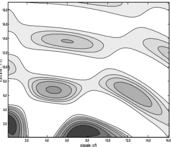
located atr′ will move toward the “source” atr′. We suppose that this is a universal property of forced con-vection and that its structures tend to approach that the centers with the strongest forcing. This structure of the Green’s function solution suggests that a spatial pattern of forced convection can be generated instantly at infi-nite distance from the source. However, as indicated by the denominator of the Green’s function, this structure decays rapidly with the distance from the source. So, in the real world, such pattern can only be expected to be observed in the adjacent region of the source. To illus-trate the effect of the cumulation of forcing at different places and times as indicated by Eq. (20), Fig. 2 gives the spatio-temporal structure of the superposition of the responses to two pulsations of forcing at (x,t )₌(0, 0) and (x,t )₌(10,₋2). A more complex structure than that in Fig. 1 can be found due to this superposition. c. Scale analysis of convective activities

x(scale: c/f)

t(

scal

e

: 1/

f)

2.0 4.0 6.0 8.0 10.0 12.0 14.0 16.0

2.0 4.0 6.0 8.0 10.0 12.0 14.0 16.0 18.0

Fig. 2. To illustrate the effect of the superposition of forcings at different places and times as indicated by Eq. (20), the figure shows the spatio-temporal structure of the superposition of the responses to two pulsations of forcing at (x,t )=(0,0) and (x,t )=(10,−2) (contour lines in divergent regions are not shown). A more complex structure can be found due to this superposition.

induced by the forcing of the vortical flow, and are es-sentially different from the inertia gravity waves.

The spatial scale of such an oscillating/propagating

structure isci/f. Sincef=10−4s−1,ci/f can either

be very small or very large, depending on the static

in-stability (or the imaginary phase speedci). This

struc-ture can be viewed as being embedded in the

synop-tic scale system whenci is small enough, otherwise it

can also be comparable to the synoptic scale whenci is

large. However, this is just the case in the situation of a vortical flow of synoptic scale. For a vortical flow of meso-scale, Eq. (13) demands the Froude number

F r_∝U/ci≪1, which gives a limitation to the lower

bound ofci. In order for the existence of Eq. (18), ci

must be large enough, otherwise the multiplicative

forc-ingℓς,φδ becomes too complex in form and cannot be

omitted and leads to a mathematical difficulty beyond the capability of the present study. In this case, the meso-scale vortical flow can induce forced convection with scales larger than the vortical flow itself. In fact, following Ford (2000), we can assume the forcing of the vortical flow to be confined to a small region with

diameterL. If the scale of the wind speed of the

vor-tical flow isU, then the scale of temporal variations is

L/U. Out of this small region, the growth rate of the

free mode of convection can be estimated by the

disper-sion relationship, i.e.λ₌

q

c2_ik2_−f2_{, where k is the}

wavenumber. We can assume that it is proportional to

L/U, or the time scale of the variation of the vortical

flow as the source of forcing. So the scale of forced

convection is 2π L/F r_≫LwhenF r_≪1.

Anyway, the scales discussed above just apply to forced convection by the imbalanced vortical flow. Free modes of convection represented by the unstable homogeneous solutions are another important factor that contributes to the spatial scales of the convective activities. Conse-quently, multiple spatial scales of convective activities are caused by the following three factors: (1) the scale of the imbalance of the vortical flow, (2) the scales of the inertial oscillation and (3) the scales of the unstable free modes of convection. Since unstable free modes of con-vection tend to select structures with the smallest scales and are embedded in the forced convection, convective activities always appear as the former modulated by the latter.

3.3 Two-way interaction between convection and vortical flow

In addition to the response of convection to the forcing in-duced by the imbalance of vortical flow as mentioned above, Eq. (15) is actually a problem of two-way interactions be-tween convective activities and the basic flow as well. The convective activities can act on the basic flow and contribute to its adjustment. In principle, this interaction between con-vection and its basic state is described by Eq. (15), although this kind of two-way interaction can never be dealt with in the framework of dynamical instabilities of basic flows.

Generally speaking, the action of the convection on the basic flow seems far more complex to describe. In the present study we would like to address this issue mathematically as below. According to the Fredholm alternative (see any text book on partial differential equation, e.g. Haberman, 2003), the solvability of Eq. (15) requires its inhomogeneous term ℜ(ς, φ)to be orthogonal to the homogeneous solutionδ0, or

< δ0,ℜ(ς, φ) >=

Z



δ∗_0ℜ(ς, φ)d₌0. (21)

Here,< , >is an inner product properly defined over some

spatiotemporal domain,δ0is the homogeneous solution of

Eq. (15) whileδ₀∗is its adjoint solution. This constraint on

ℜ(ς, φ)means that the departure from balance is confined to merely some very special ways. It can then be explained as the action of convection on its basic flow. Since the

ho-mogeneous solutionδ0represents all possible free modes of

convection, this reaction adjusts the basic flow in a

particu-lar way so that the resulting forcingℜ(ς, φ)has no

which may be essentially a limitation to the further

intensifi-cation of the forcing_ℜ(ς, φ), or roughly, a measure for the

imbalance. So, the imbalance of the vortical flow cannot in-crease infinitely and an approximately balanced flow can be maintained.

A more physical explanation for this action of convection on the basic flow can be obtained from an approximate anal-ysis of the Green’s function (19). The inhomogeneous solu-tion of convecsolu-tion far apart from the “source” of the

imbal-ance can be estimated by setting the “source” atr′=0 and

t′₌0 in the Green’s function. So, we have

δn(r, t )∝Re(aeiθ)=acos(θ ), (22)

where the “phase” is given by

θ₌f ci

q

|r|2_+c2

it2 (23)

The amplitudeavaries slowly withtand r and is assumed to

be constant. On the other hand, out of the “source” region,

we haveℜn(ς, φ)=0, so the governing equation should be

∂2δn ∂t2 +c

2

i∇2δn+f2δn=0 (24)

although the inhomogeneous solution is considered.

Multi-plying Eq. (24) by∂δn∂t, we have the following

conserva-tion law of Eq. (24)

∂

∂t(

1

2δ

2 nt−

1

2c

2 i|∇δn|

2 +1

2f

2_δ2

n)+ ∇ ·(c2iδnt∇δn)=0. (25)

By substituting Eqs. (22) and (23) into Eq. (25) and

integrat-ing fromθ₌0 toθ₌2π, we rewrite Eq. (25) as

∂E

∂t + ∇ ·F=0., (26)

Here,

E₌ f

2_c2 it2a2

2(_|r|2_+c2

it2)

(27a)

F₌ f

2_c2 it a

2

2(_|r_|2_+c2

it2)

r (27b)

are the energy density and flux, respectively. The group ve-locity which indicates the wave energy transportation can be obtained by

cg=

F

E=

1

tr. (28)

It clearly demonstrates that outward and temporally de-caying energy transportation from the “source” accompanies the imbalance, which will essentially reduce the convection

orδand tends to maintain the balance of the basic flow. The

fact that the group velocity goes to infinity whent goes to 0

does not need to mean that there is no point unaffected by the

“source”, because the energy densityEas well as the fluxF

vanish, i.e. there is no transport of energy. On the contrary, the local phase speed is given by

c=−∂θ/∂t ∂θ/∂x i+

−∂θ/∂t ∂θ/∂y j= −

c2_it

|r|2r, (29)

This phase propagation toward the “source” has been demon-strated in Fig. 1. So, we can conclude that the two-way in-teraction between convection and its basic state is character-ized by the following process: the imbalance of the basic flow generates convection, while the convection suppresses the further increase of this imbalance in turn.

3.4 Physical explanation and observational evidences

In order to identify spontaneous convection as described above in the real world, two fundamental aspects, i.e. un-stable stratification and imbalance of the basic state should be observed simultaneously. The unstable stratification gen-erates small cells of convection, while the imbalance gives a larger-scale modulation with spatio-temporal structures indi-cated by Eq. (20). In fact, since no exactly balanced flow can be found in the atmosphere and unstable stratification is also very common, most of the convective activities have some-thing to do with this spontaneous convection.

For the purpose above, we need also an explanation of the

physical meaning of the imbalance forcingℜ(ς, φ). If the

vertical or horizontal structures of the terms in brackets in ℜ(ς, φ)are approximately sine or cosine functions, the

im-balance forcing can be viewed as the result of(a_ς2₊b_ς2₋ς2)t

(nonsteady processes of the vortical flow),Vς·∇ς(vorticity

advection) and[Vς· ∇(∂φ_∂p)]p(difference of temperature

) 2 ( ) 1 (

n n

n

δ

δ

δ

=

+

) , ( 1

2 2 2 2 2 2 2 2 2

φ ς δ

τ δ δ δ

n i n i n n n

c c f y

x ∂ + = ℜ

∂ + ∂ ∂ + ∂ ∂

Homogeneous solution: apparent static instability

Inhomogeneous solution: Forced convection

Act on basic flow? ) , (

2 2 2 2

φ ς δ δ σ δ

ℜ = + ∇ + ∂ ∂

pp pp

f t

NO YES

Synoptic scale or

meso-scale with Fr << 1

For vertical modes with unstable stratification

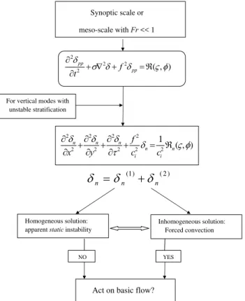
Fig. 3.A schematic overview about the different cases discussed in Sect. 3.

convection. A particular case for convection without large or meso-scale synoptic systems accompanied is daytime heat-ing on a flat and homogeneous surface. In this case, the

ba-sic flow is nearly balanced and_ℜ(ς, φ)remains very small.

Once the stratification of the atmosphere becomes unstable, the unstable free modes dominate over the forced part of con-vection. Although imbalance may be too weak to generate a noteworthy part of convection, it can still provide an initial disturbance from which instability develops spontaneously. Although the forcing terms are very similar to those of the

well-knownωequation (see, e.g. Holton, 1992), it is worthy

to mention that the forced part of convection is essentially different from the issue of vertical motion generated from

vortical flow as described by theωequation. If the

atmo-sphere is stably stratified (σ >0), the ωequation is an

el-liptic equation. To the leading order, it describes the spon-taneous emission of inertia gravity waves in the “source” region. However, if the atmosphere is unstably stratified (σ <0),ωequation becomes a hyperbolic equation and usu-ally not to be used for the diagnosis of the vertical motion.

So, the vertical motion forσ <0 remains unclear so far, and

the present concept of forced convection can’t be attributed to the conventional vertical motion. In other words, it is the way of response rather than the form of forcing that is different. A schematic overview about the different cases discussed in this section is given in Fig. 3.

4 Conclusions and discussions

The present study suggests that convective activities can be recognized in the perspective of their interaction with the vortical flow. It has been demonstrated that convective ac-tivities can be regarded as the superposition of free modes of convection and the response to the forcing induced by the imbalance of the unstably stratified vortical flow. An im-balanced vortical flow provides not only an initial condition from which unstable free modes of convection can develop but also a forcing on the convection. Soconvection is more appropriately to be regarded as a spontaneous phenomenon rather than a disturbance-triggered phenomenon which is in-dicated by any theory of dynamical instability. Meanwhile, convection, particularly the forced part, has also a reaction on the basic flow by preventing the imbalance of the vortical flow from further increase and maintaining approximately a balanced flow.

It is crucial to make clear how the proposed point of view could improve the classical description of convection. The key point is that, by introducing the framework of balanced flows, it extends previous theories which attribute convec-tion mainly to dynamical instabilities of the balanced basic state. The presented theory considers not only the apparent instabilities but also the interaction of convective activities with the imbalanced basic state. Moreover, the basic state can now be much more complex than in traditional theory. These differences need not to increase the difficulties in the analysis of the apparent instability and the interaction when

ℓς,φδis dropped just as in Sect. 3.

disparate to allow convection to directly affect the larger-scale flow. This is a central assumption in the statistical quasi-equilibrium hypothesis (SQE), which is not opposite to our conjecture that convection serves to adjust the larger-scale environment to a state of balance. What Emanuel et al., mean by convection corresponds just to the free modes of convection or the homogeneous solution that is not related to the vortical flows in the linear stage of growth. On the contrary, the forced part of convection or the inhomogeneous solution does serve to adjust the larger-scale environment as was pointed in last section. Such a discrepancy is just due to the difference of definitions of convection and is not sig-nificant for larger-scale vortical flow. But for smaller-scale vortical flows with strong imbalance, this discrepancy may become important.

Another question may also arise from this difference of definitions of convection, that is, the larger-scale environ-ment always has regions of convergence/divergence of the same scale, while a vortical flow associated with the forc-ing _ℜ(ς, φ) is always nondivergent. This can simply be explained because in the generalized definition these larger-scale convergence/divergence is included in the convection rather than in its environment. It is also easy to see that the friction and diabatic heating can be incorporated into the present framework without technical difficulty. As a result, the effects of the physical boundary layer and latent heating on convections can be discussed within this framework as well, which will be the topic of our future investigations on this issue. We believe these theoretical results on balanced circulations with convective activity can provide a new per-spective for diagnostic studies to understand the formation and the structure of meso-scale convection systems.

Appendix A

LetLdenote the linear operator in the left-hand side of (15),

i.e.

L_{= −}d

2

dp2 (A1)

Then the eigen-system (15) can be written as

LPn=λnσ Pn; n=0,1,2, ... (A2)

It may satisfy the following boundary conditions of the

first, second and third kinds atp₌0 andps:

α1Pn(0)+β1Pn′(0)=0

α2Pn(ps)+β2Pn′(ps)=0. (A3)

Here,_|α1|2+ |β1|26=0; |α2|2+ |β2|26=0. We define the

inner product by

< u,v >₌

Z ps

0

u∗vdp. (A4)

It is easy to prove that

< Pn, LPn>−< LPn, Pn>=(λn−λ∗n)

Z p0

0

σ_|Pn|2dp. (A5)

And by multiplying Eq. (A2) byP_n∗, we have also

λn

Z p0

0

σ_|P_n|2dp_{= −}Pn dP_n∗

dp

p0

0 +

Z p0

0

dPn dp

2

dp. (A6)

SinceLis a self-adjoint operator and the first term of the

right hand side of Eq. (A6) is non-negative under any of the boundary conditions of Eq. (A3), for an arbitrary nontrivial solution of Eq. (A2), we have

(λn−λ∗n)

Z p0

0

σ_|Pn|2dp=0 (A7a)

λn

Z p0

0

σ_|P_n|2dp >0. (A7b)

For a certain eigenfunctionPn, we can define an equivalent

parameter of static stability by the weighted average ofσ

over the entire layer of the atmosphere, i.e.

σn=

Z p0

0

σ_|P_n|2dp (A8)

where the weight is chosen as the power of the normalized

Pn. It can be inferred from Eq. (A7a and b) that, ifσn>0

(σn<0),λn is real andλn>0 (λn<0). A special case is

when σ >0(σ <0)at all levels. In other words, if the

at-mosphere is statically stable, thenλn>0 holds for all

eigen-functions. Otherwise, if the atmosphere is statically unstable

at some layer, it is assumed that we can find someλn<0, a

particular case of which is all theλn<0 whenσ <0, or the

atmosphere is statically unstable at the whole layer.

It is necessary to specify the vertical boundary condition

suitable for the present issue from Eq. (A3). By lettingα1=0

and β2/α2>0 in Eq. (A3), the eigen-system satisfies the

second and the third kind of boundary conditions atp₌0

andps, respectively. The physical meanings of these

bound-ary conditions are also clear: there is no exchange of gence at the top of the atmosphere, and exchange of conver-gence at surface is proportional to the converconver-gence in situ.

Acknowledgements. The authors are grateful to R. Donner and two anonymous referees for their insightful comments and suggestions. This study is supported by the National Natural Science Foundation of China under Grant No. 41175065 and 41075039 and, the Chinese Special Scientific Research Project for Public Interest under Grant No. GYHY200806009, GYHY201206038, and the Qinglan Project of Jiangsu Province of China under Grant No. 2009.

Edited by: R. Donner

References

Arakawa, A. and Schubert, W. H.: Interaction of a cumulus cloud ensemble with the large-scale environment, Part I., J. Atmos. Sci., 31, 674–701, 1974.

Charney, J. G.: The use of the primitive equation of motion in nu-merical prediction, Tellus, 7 22–26, 1955.

Drazin, P. G.: Hydrodynamical stability, Cambridge University Press, Cambridge, 1981.

Emanuel, K. A., Neelin, J. D., and Bretherton, C. S.: On large-scale circulations in convecting atmospheres, Quart. J. Roy. Met. Soc., 120, 1111–1143, 1994.

Ford, R., McIntyre, M. E., and Norton, W. A.: Balance and the slow quasimanifold: Some explicit results, J. Atmos. Sci., 57, 1236– 1254, 2000.

Guo, D. R.: Methods of Mathematical Physics, People’s Education Press, Beijing, 1979 (in Chinese).

Haberman, R.: Applied Partial Differential Equations, 4th Edn., Prentice Hall, 2003.

Holton J. R.: An introduction to dynamic meteorology, Academic Press, 1992.

Hoskins, B. J.: The role of potential vorticity in symmetric stability and instability, Quart. J. Roy. Meteor. Soc, 100, 480–482, 1974. Jacobs, S. J.: On the existence of a slow manifold in a model system

of equations, J. Atmos. Sci., 48, 793–801, 1991.

Leith, C. E.: Nonlinear normal mode initialization and quasi-geostrophic theory, J. Atmos. Sci., 37, 958–968, 1980.

Lighthill, M. J.: On sound generated aerodynamically, I. General theory, Proc. Roy. Soc. London, Ser. A, Math. Phys. Sci., 211, 564–587, 1952.

Lorenz, E. N.: Attractor sets and quasi-geostrophic equilibrium, J. Atmos. Sci., 37, 1685–1699, 1980.

Lorenz, E. N.: On the existence of a slow manifold, J. Atmos. Sci., 43, 1547–1557, 1986.

Lorenz, E. N. and Krishnamurthy, V.: On the nonexistence of a slow manifold, J. Atmos. Sci., 44, 2940–2950, 1987.

Lorenz, E. N.: The Slow Manifold – What Is It?, J. Atmos. Sci., 49, 2449–2451, 1992.

Lynch, P.: The slow equations, Q. J. Roy. Meteor. Soc., 115, 201– 219, 1989.

McIntyre, M. E.: Balance, potential-vorticity inversion,

Lighthill radiation, and the slow quasimanifold, Proc. IU-TAM/IUGG/Royal Irish Academy Symposium on Advanced in Mathematical Modelling of Atmosphere and Ocean held at the Univ. of Limerick, Ireland, 2–7 July 2000, edited by: Hodnett, P. F., 45–68, 2000.

Moura, A. D.: The Eigensolutions of the Linearized Balance Equa-tions over a Sphere, J. Atmos. Sci., 33, 877–907, 1976. Pedlosky, J.: Geophysical Fluid Dynamics, Springer Verlag, New

York, 1979.

de Roode, S. R., Duynkerke, P. G., and Jonker, H. J. J.: Large eddy simulation: How large is large enough?, J. Atmos. Sci., 61, 403-421, 2004.

Vallis, G. K.: Potential vorticity and balanced equation of motion for rotating and stratified flows, Q. J. Roy. Met. Soc., 122, 291– 322, 1996.

Vanneste, J. and Yavneh, I.: Exponentially Small Inertia–Gravity Waves and the Breakdown of Quasigeostrophic Balance, J. At-mos. Sci., 61, 211–223, 2004.

Vautard, R. and Legras, B.: Invariant manifolds, quasi-geostrophy and initialization, J. Atmos. Sci., 43, 565–584, 1986.

Warn, T.: Nonlinear balance and quasi-geostrophic sets, Atmos. Ocean., 35, 135–145, 1997.

Warn, T. and Menard, R.: Nonlinear balance and gravity-inertia wave saturation in a simple atmospheric model, Tellus, 38A, 285–294, 1986.

Warn, T., Bokhove, O., Shepherd, T. G., and Vallis, G. K.: Rossby number expansions, slaving principles, and balance dynamics, Q. J. Roy. Met. Soc., 121, 723–739, 1995.

Williams, P. D., Haine, T. W. N., and Read, P. L.: Inertia-Gravity Waves Emitted from Balanced Flow: Observations, Properties, and Consequences, J. Atmos. Sci., 65, 3543–3556, 2008. Xu, Q. and Clark, J. H. E.: The Nature of Symmetric Instability

and Its Similarity to Convective and Inertial Instability, J. Atmos. Sci., 42, 2880–2883, 1985.