SRef-ID: 1432-0576/ag/2004-22-2973 © European Geosciences Union 2004
Annales
Geophysicae
Cosmic radio-noise absorption bursts caused by solar wind shocks
A. Osepian1and S. Kirkwood2
1Polar Geophysical Institute, Halturina 15, Murmansk, Russia 2Swedish Institute of Space Physics, Box 812, 98128 Kiruna, Sweden
Received: 14 October 2003 – Revised: 7 April 2004 – Accepted: 20 April 2004 – Published: 7 September 2004
Abstract. Bursts of cosmic noise absorption observed at times of sudden commencements (SC) of geomagnetic storms are examined. About 300 SC events in absorption for the period 1967–1990 have been considered. It is found that the response of cosmic radio-noise absorption to the passage of an interplanetary shock depends on the level of the plan-etary magnetic activity preceding the SC event and on the magnitude of the magnetic field perturbation associated with the SC (as measured in the equatorial magnetosphere). It is shown that for SC events observed against a quiet back-ground (Kp<2), the effects of the SC on absorption can be
seen only if the magnitude of the geomagnetic field pertur-bation caused by the solar wind shock exceeds a threshold value1Bth. It is further demonstrated that the existence of
this threshold value,1Bth, deduced from experimental data,
can be related to the existence of a threshold for exciting and maintaining the whistler cyclotron instability, as predicted by quasi-linear theory. SC events observed against an active background (Kp>2) are accompanied by absorption bursts
for all magnetic field perturbations, however small. A quan-titative description of absorption bursts associated with SC events is provided by the whistler cyclotron instability the-ory.
Key words. Ionosphere (physics particle precipitation; wave particle interaction) – Magnetospheric physics (storms and substorms)
1 Introduction
Electron fluxes precipitating into the auroral region often show a variety of time structures. The temporal scale of the variations is from fractions of a second to several hundred seconds. Most published studies of the nature of impulsive electron bursts and electron-flux pulsations have suggested explanations based on the theory of whistler cyclotron insta-bility (Coroniti and Kennel, 1970; Davidson and Chiu, 1986; Correspondence to:S. Kirkwood
Trakhtengerts et al., 1986; Demekhov and Trakhtengerts, 1994; Demekhov et al., 1998; Manninen et al., 1996).
The properties of non-stationary regimes of whistler cy-clotron instability which exist in the presence of a constant free energy source (e.g. injection of energetic electrons or local acceleration mechanisms) were investigated by Trakht-engerts et al. (1986), Demekhov and TrakhtTrakht-engerts (1994), Demekhov et al. (1998). A self-exciting model of a whistler cyclotron maser derived from the full set of quasi-linear equations, valid for weak-to-moderate pitch angle diffusion, was developed by these authors to explain certain types of impulsive energetic electron precipitation and auroral elec-tron precipitation pulsations. These types of precipitation have periods of several tens of seconds and are observed in situations where magnetic field variations with the time scales of interest are absent in the equatorial region of the magnetosphere.
0.40 0.60 0.80 1.00 0.5
0.0 1.0
A,
d
B
04.10.1978 SC 0045 UT
13.40 13.60 13.80 14.00 14.20 0.5
1.5
0.0 1.0
A,
dB
31.10.1981 SC 1338 UT
23.40 23.60 23.80 24.00
Time, UT 0.5
1.5 2.5
0.0 1.0 2.0
A, dB
25.06.1974 SC 2329 UT
SC
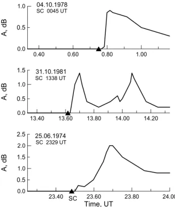
Fig. 1a. Cosmic noise absorption bursts (SCA) caused by solar wind shocks in different local time sectors. Planetary magnetic ac-tivity preceding the SC events is low (4 October 1978 –Kp=2−; 31 October 1981 –Kp=1−, 25 June 1974 –Kp=1+). The time of the SC is indicated by the black triangle.
perturbation is introduced into the magnetic field, have been derived by Coroniti and Kennel (1970) and Perona (1972) and used to investigate temporal changes in the wave growth rate and diffusion coefficient. Both models take into ac-count adiabatic changes in the pitch-angle anisotropy index A. However, the fraction of the distribution in resonance,η, is assumed to be constant.
Impulsive bursts of VLF emissions associated with the sudden commencement (SC) of geomagnetic storms or with sudden impulses (SI) have been observed by satellites (Kokubun, 1983; Gail and Inan, 1990) at L-shells in the range of 3<L<6 and at ground-based stations at auroral and sub-auroral latitudes (Morozumi, 1965; Hayashi et al., 1968; Kleimenova and Osepian, 1982; Gail et al., 1990; Yahnin et al., 1995; Manninen et al., 1996). Gail et al. (1990) reported that changes in VLF wave activity at high-latitude stations were observed in 50–60% of the events studied and for 80% of the events when the observing station was on the day or morning side of the Earth. Spacecraft data have shown that wave growth is observed on the nightside as well as the day-side, and no clear local time dependence was found (Gail and Inan, 1990). As shown by Gail et al. (1990) the abil-ity of the model suggested by Perona (1972) to predict the observed changes in the properties of diffuse emissions dur-ing SCs (growth rate, growth time and total growth) is quite reasonable.
2.00 2.20 2.40 2.60 2.80 3.00 0.5
1.5
0.0 1.0
A,
dB
11.11.1979 SC 0225 UT
5.00 5.20 5.40 5.60 5.80 0.5
1.5
0.0 1.0
A, dB
22.10.1981 SC 0524 UT
10.60 10.80 11.00 11.20 11.40
Time, UT
0.5 1.5 2.5 3.5
0.0 1.0 2.0 3.0
A,
d
B
13.04.1983 SC 1100 UT
Fig. 1b. Cosmic noise absorption bursts (SCA) caused by solar wind shocks in different local time sectors. Planetary magnetic activity preceding the SC events is high (11 November 1979 – Kp=3−; 22 October1981 –Kp=4−; 13 April 1983 –Kp=3). The time of the SC is indicated by the black triangle.
First observations of the SC effect in ionospheric ab-sorption were described by Brown et al. (1961). Ortner et al. (1962) reported that ionospheric absorption during SCs was located around the maximum of the auroral zone and was rarely observed at sub-auroral geomagnetic latitudes. Kleimenova and Osepian (1982) and Gail et al. (1990) ob-served cases of simultaneous bursts in VLF emissions and ionospheric absorption associated with SC events. Increased electron density at altitudes 80–100 km has also been de-tected by the EISCAT incoherent-scatter radar during several SC events (Yahnin et al., 1995; Manninen et al., 1996).
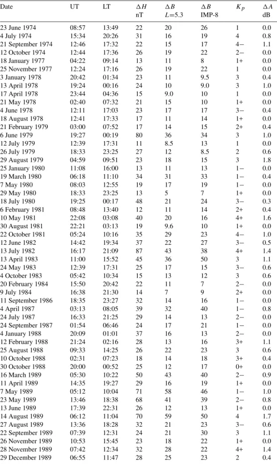
Table 1.Dates, times (UT and LT), magnitudes (1H,1Band1A) and background magnetic acticity (Kp) for a representative subset of the events analysed.
Date UT LT 1H 1B 1B Kp 1A
nT L=5.3 IMP-8 dB
23 June 1974 08:57 13:49 22 20 26 1 0.0
4 July 1974 15:34 20:26 31 16 19 4 0.8
21 September 1974 12:46 17:32 22 15 17 4− 1.1
12 October 1974 12:44 17:36 26 19 22 2− 0.0
18 January 1977 04:22 09:14 13 11 8 1+ 0.0
25 November 1977 12:24 17:16 26 19 22 1 0.0
3 January 1978 20:42 01:34 23 11 9.5 3 0.4
13 April 1978 19:24 00:16 24 10 9.0 3 1.0
17 April 1978 23:44 04:36 15 9.0 10 1 0.0
21 May 1978 02:40 07:32 21 15 10 1+ 0.0
4 June 1978 12:11 17:03 23 17 17 3− 0.4
18 August 1978 12:41 17:33 17 11 14 1+ 0.0
21 February 1979 03:00 07:52 17 14 15 2+ 0.4
6 June 1979 19:27 00:19 80 36 34 3 1.0
12 July 1979 12:39 17:31 11 8.5 13 1 0.0
26 July 1979 18:33 23:25 27 12 8.5 2 0.6
29 August 1979 04:59 09:51 23 18 15 3 1.8
25 January 1980 11:08 16:00 13 11 13 1− 0.0
19 March 1980 06:18 11:10 34 31 33 1− 0.4
7 May 1980 08:03 12:55 19 17 19 1− 0.0
29 May 1980 18:33 23:25 13 5 7 1+ 0.0
18 July 1980 19:25 00:17 48 21 24 3− 0.3
6 February 1981 08:48 13:40 12 11 14 2+ 0.4
10 May 1981 22:08 03:08 40 20 16 4+ 1.6
30 August 1981 22:21 03:13 19 9.6 10 1+ 0.0
22 October 1981 05:24 10:16 35 29 23 4− 1.0
12 June 1982 14:42 19:34 37 22 27 3− 0.5
13 July 1982 16:17 21:09 87 43 38 4+ 1.4
13 April 1983 11:00 15:52 45 36 50 3 1.1
24 May 1983 12:39 17:31 25 17 15 3− 0.6
4 October 1983 05:42 10:34 15 13 12 3 0.6
20 February 1984 15:50 20:42 22 11 7 2− 0.0
9 July 1984 16:38 21:30 14 7 9 2+ 0.0
11 September 1986 18:35 23:27 32 14 16 1− 0.0
4 April 1987 03:13 08:05 39 32 40 1− 0.8
24 July 1987 16:33 21:25 29 14 13 2− 0.0
24 September 1987 01:54 06:46 24 17 21 1− 0.0
4 January 1988 20:09 01:01 37 16 13 2− 0.0
12 February 1988 21:24 02:16 28 13 16 3+ 1.1
25 August 1988 09:33 14:25 26 22 23 3 0.6
10 October 1988 02:31 07:23 18 14 18 3+ 0.4
30 October 1988 20:00 00:52 25 12 17 0+ 0.0
16 March 1989 05:30 10:22 50 43 40 2− 0.9
11 April 1989 14:35 19:27 29 16 19 1+ 0.0
7 May 1989 05:12 10:04 71 58 46 1− 1.0
23 May 1989 13:46 18:38 68 41 39 2− 0.8
13 June 1989 17:39 22:31 26 12 13 1+ 0.0
14 August 1989 06:12 11:04 70 59 50 4 1.7
27 August 1989 13:36 18:28 32 21 23 3− 0.6
22 September 1989 07:39 12:31 24 21 30 3 1.1
26 November 1989 10:53 15:45 23 18 22 1+ 0.0
28 November 1989 07:42 12:34 32 28 22 4+ 1.4
20.00 20.50 21.00
Time, UT
0.5
0 1
A, dB
20.00 20.50 21.00
Time, UT
f = 760 Hz
20.00 20.50 21.00
Time, UT
f = 1200 Hz 19.03.1969
19.03.1969
19.03.1969 SC 1958 UT
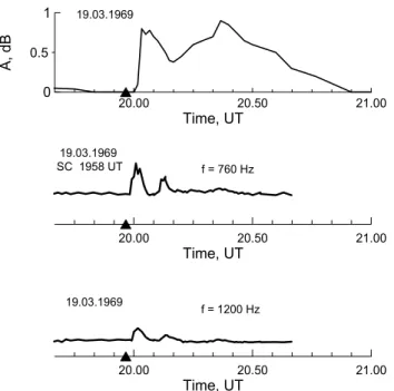
Fig. 2a. Cosmic noise absorption (SCA) and bursts of VLF-emission observed on 19 March 1969. Planetary magnetic activity preceding the SC event is low (Kp=1+). The time of the SC is indicated by the black triangle.
9.80 10.00 10.20 Time, UT
0.5
0.0 1.0
A, d
B
9.80 10.00 10.20 Time, UT
f = 2525 Hz 05.11.1973
05.11.1973 SC 0952 UT
Fig. 2b.Cosmic noise absorption (SCA) and burst of VLF-emission observed on 5 November 1973. Planetary magnetic activity preced-ing the SC event is high (Kp=3). The time of the SC is indicated by the black triangle.
in the Appendix. In Sect. 2 we show that the SC effect in ionospheric absorption depends on the pre-history or the state of the magnetosphere before the SC event. In Sects. 3 and 4 we investigate temporal changes in the anisotropy index, the wave growth rate and the pitch-angle diffusion caused by a perturbation1B. We use the approach to this problem de-scribed by Coroniti and Kennel (1970) and Perona (1972). We take into account changes in all parameters included in the equation for wave growth, including changes in the frac-tion of resonant electrons,η, due to adiabatic changes and
0 10 20 30 40 50 60 70 80 90 100
∆
B, nT
0
1
2
3
4
5
6
∆
A,
d
B
Kp<2
0
10
20
30
40
50
60
70
80
∆
B, nT
0
1
2
3
4
5
6
∆
A,
d
B
Kp
>2-Fig. 3. Magnitude of the impulse in cosmic noise absorption1A as a function of the magnetic impulse1Binduced by the SC at the magnetic equator atL=5.3. The upper panel is for quiet conditions (Kp<2) preceding the SC, the lower panel is for active conditions (Kp≥2).
acceleration of hot particles in the induction electric field. In Sect. 3 we estimate the time delay of absorption bursts relative to the magnetic impulse associated with the SC for SC events observed against a quiet background (Kp<2). We
also estimate the value of perturbation1B in the magnetic field strength required to generate whistler cyclotron insta-bility against a background corresponding to a quiet magne-tosphere. In Sect. 4 we determine relative changes in pitch-angle diffusion coefficientD∗caused by SC events observed against an active background (Kp≥2) and predict changes in
absorption value during real SC events.
2 Experimental data
using riometer records obtained at the station Loparskaya (8=64◦N,3=115.5◦E,L=5.3) for the period 1967–1990. We excluded from consideration all cases when the SC was observed against a background of solar proton precipitation (solar proton events, SPE). As a result, 352 of the SC events registered by magnetic stations for 1967–1990 are included in our study. We find that the response of cosmic radio-noise absorption to the passage of the bow shock depends on the level of the planetary magnetic activity (Kpindex) preceding
the SC. From the 352 SC events considered, only 190 cases are accompanied by bursts of SCA. For 174 SC events ob-served against a quiet background (Kp<2), effects of the SC
are seen in absorption only for 33 cases (18.9%). For 178 SC events observed against an active background (Kp≥2) bursts
in absorption are observed on 157 occasions (88.2%). Exam-ples of SCA bays during SC observed against backgrounds of both low and high activity are shown in Figs. 1a, b.
Figure 2a shows records of SCA in Loparskaya and VLF bursts observed in Sogra (8′=56.6◦N,3=124◦E,L=3.7) at the time of the SC on 19 March 1969 at 19:58 UT (plan-etary magnetic activity before the SC is low,Kp=1+).
Fig-ure 2b presents SCA in Loparskaya and VLF emission ob-served in Lovozero (8′=63.8◦N,3=127◦E,L=5.1) at the time of the SC on 5 November 1973 at 09:52 UT (Kp=3
preceding the SC in this case). It can be seen that for the SC observed against a quiet background (Figs. 1a, 2a), there is a short (about 30–60 s) delay of the SCA bay and VLF burst relative to the SC. In active periods, absorption and VLF emission increase together with the SC (Figs. 1b, 2b). Figure 3 shows the relationship between the magnitude of absorption bursts and of the magnetic impulse1B induced by the SC in the equatorial magnetosphere atL=5.3. The upper panel is for quiet conditions (Kp<2) preceding the
SC; the lower panel is for active conditions (Kp≥2). The
method of determining1Bis described in the Appendix. It is clear that in the quiet case absorption bursts are observed only when the perturbation1B exceeds a threshold value 1Bt h≈30 nT. In the disturbed case almost all SC events,
in-cluding very small perturbations, are accompanied by bursts in absorption.
3 Magnetic field perturbation 1B needed to excite whistler cyclotron waves atL=5.3
In this section we show that properties of absorption bursts (SCA), such as the dependence of occurrence onKp
preced-ing the SC event, the threshold value1Bthand the time delay
of SCA relative to the SC, can be predicted in the context of the whistler cyclotron instability theory.
We first give a brief review of the whistler cyclotron insta-bility theory. Growth and damping of whistler mode waves with frequencyωare controlled by the characteristics of the ambient magnetospheric plasma (hot and cold plasma den-sity, pitch-angle distribution function, fraction of resonant electrons) which change depending on the level of planetary magnetic activity. It is generally expected that pre-conditions
must be satisfied in order to produce wave growth. The tem-poral growth rateγ of whistler waves at frequencyωderived by Kennel and Petschek (1966 ) is
γ =π eη(Eres)
{A−(Eres)−1/[(e/ω)−1]}{1−(ω/ e)}2, (1)
whereeis the electron gyrofrequency; Eres=meVres2 /2 is
the parallel electron energy required for Doppler-shifted cy-clotron resonance with whistler mode waves at frequencyω, meis the electron mass;Bois the magnetic field in the
equa-torial plane, A−(Eres)is the index of electron pitch-angle
anisotropyη(Eres)is the fraction of the total particle
distri-bution which satisfies the resonance condition (its exact def-inition is given by Kennel and Petchek, 1966). η(Eres)is
related to the omnidirectional fluxJ2π(E≥Eres), which is
an observed quantity, by the following relation:
η(Eres)=J2π(E≥Eres) , /2VresN (1a)
whereN is the cold plasma density.
Sinceη(Vres)is always positive, the wave grows (γ >0) if
the anisotropyA−(Eres)is greater than a critical value A−c
which is frequency dependent
A−(Eres)c= {(e/ω)−1}−1. (1b)
The maximum initial frequencyωmoof unstable (γ≥0)
cy-clotron waves is determined by the following inequality ωmo< A−0e/(1+A−0)≪e, (2)
whereA−0 is a initial anisotropy.
For instability to be self-sustaining, the total amplifica-tion of whistler waves on one pass between conjugate iono-spheres must compensate the wave losses due to reflection at the magnetosphere-ionosphere interface. Mathematically, the condition required to maintain self-exciting waves is presented in the following form (Cornilleau-Wehrlin et al., 1985; Demekhov and Trakhtengerts, 1994):
Ŵ=
Z
γ dS/Vg≥ |ln 1/R| or
γ ≥γt h=ν≡(Vg/LRe)|lnR|, (3)
where ν is the loss rate of the wave energy, R is the ef-fective reflection coefficient from the ionosphere. The re-flection coefficient R is difficult to evaluate. As a rule, the numerical value |ln 1/R| is assumed to be equal to 3 (Cornilleau-Wehrlin et al., 1985; Schulz and Davidson, 1988). Vg=2Bo/(4π meN )1/2(ω/ e)1/2(1−ω/ e)3/2 is
the equatorial group velocity of the wave at a givenL-shell; dSis the increment of the magnetic field line length;l≈LRE
is the resonator length between the reflection points on the given magnetic field line;REis the radius of the Earth.
The condition (3)is satisfied in that region of the mag-netosphere where the temporal growth rate is positive and there are enough electrons near resonance, i.e. the total flux of trapped electronsJ (E≥Eres)exceeds the threshold
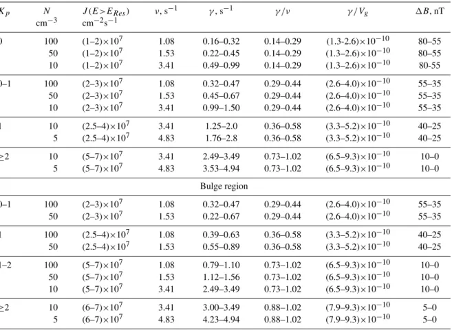
Table 2.Calculated parameters of whistler wave growth at various levels of planetary magnetic activity (Kp). Plasma density (N) and flux of energetic electrons (J) are assumed parameters. The calculated parameters are temporal growth rate (γ), spatial growth rate (γ /Vg), loss rate (ν) and the minimum jump in magnetic field (1B) needed to raise the growth-rate to the level where it exceeds the critical value estimated by Cornilleuau-Werlin et al. (1985)(all calculations forL=5.3,ω/ e=0.12,A−0=0.3, ln(1/R)=3.
Kp N J (E>ERes) ν, s−1 γ, s−1 γ /ν γ /Vg 1B, nT
cm−3 cm−2s−1
0 100 (1–2)×107 1.08 0.16–0.32 0.14–0.29 (1.3-2.6)×10−10 80–55
50 (1–2)×107 1.53 0.22–0.45 0.14–0.29 (1.3–2.6)×10−10 80–55
10 (1–2)×107 3.41 0.49–0.99 0.14–0.29 (1.3–2.6)×10−10 80-55
0–1 100 (2–3)×107 1.08 0.32–0.47 0.29–0.44 (2.6–4.0)×10−10 55–35
50 (2–3)×107 1.53 0.45–0.67 0.29–0.44 (2.6–4.0)×10−10 55–35
10 (2–3)×107 3.41 0.99–1.50 0.29–0.44 (2.6–4.0)×10−10 55–35
1 10 (2.5–4)×107 3.41 1.25–2.0 0.36–0.58 (3.3–5.2)×10−10 40–25
5 (2.5–4)×107 4.83 1.76–2.8 0.36–0.58 (3.3–5.2)×10−10 40–25
≥2 10 (5–7)×107 3.41 2.49–3.49 0.73–1.02 (6.5–9.3)×10−10 10–0
5 (5–7)×107 4.83 3.53–4.94 0.73–1.02 (6.5–9.3)×10−10 10–0
Bulge region
0–1 100 (2–3)×107 1.08 0.32–0.47 0.29–0.44 (2.6–4.0)×10−10 55–35
50 (2–3)×107 1.53 0.22–0.67 0.29–0.44 (2.6–4.0)×10−10 55–35
1 100 (2.5–4)×107 1.08 0.39–0.63 0.36–0.58 (3.3–5.2)×10−10 40–25
50 (2.5–4)×107 1.53 0.55–0.89 0.36–0.58 (3.3–5.2)×10−10 40–25
1–2 100 (5–7)×107 1.08 0.79–1.10 0.73–1.02 (6.5–9.3)×10−10 10–0
50 (5–7)×107 1.53 1.12–1.56 0.73–1.02 (6.5–9.3)×10−10 10–0
10 (5–7)×107 3.41 2.49–3.49 0.73–1.02 (6.5–9.3)×10−10 10–0
≥2 10 (6–7)×107 3.41 3.00–3.49 0.88–1.02 (7.9–9.3)×10−10 5–0
5 (6–7)×107 4.83 4.23–4.94 0.88–1.02 (7.9–9.3)×10−10 5–0
Schulz and Davidson, 1988). A critical value for the spatial growth rateγ /Vgis estimated to beγt h/Vg≈1×10−9cm−1
(Cornilleau-Wehrlin et al., 1985).
In Table 2 we present quantitative evaluations of the tem-poral (γ) and spatial (γ /Vg)growth rates and the loss rate
(ν) calculated for the equatorial plane atL=5.3 for differ-ent levels of planetary magnetic activity. We assume that reduced resonant frequency x=ω/ e=0.12−0.15,
magni-tude of anisotropy indexA−(Eres)=0.3 and resonant energy Eres=30 keV are the most realistic plasma parameters in the
equatorial magnetosphere atL=5−6 (Cornilleau-Wehrlin et al., 1985; Kirkwood and Osepian, 2001).
We also need to use realistic values of the cold plasma density (N) and trapped electron fluxesJ (E≥30 keV). Large numbers of measurements have been obtained with satellites near the equatorial plane atL=5.0−5.5. It is well estab-lished that there is a region of sharp gradient in the dis-tribution of the cold plasma density in the magnetosphere – the plasmapause – where the plasma density decreases by 1–2 orders of magnitude. The location of the plasma-pause,LP , depends on the level of magnetic activity and
on the MLT sector (Carpenter, 1967; Binsak, 1967;
Chap-pel et al., 1970a; ChapChap-pel et al., 1970b; Harris et al., 1970; Rycroft and Thomas, 1970; Chappel et al., 1971; Park et al., 1978; Singh and Horwitz, 1992). As a rule, the L -shell=5.3 is located outside the plasmasphere (LP<5.3) if
the Kp index is about 1 or higher. In these cases we take
values N=10−5 cm−3 to evaluate the increment, the loss
rate and the spatial (γ /Vg)growth rate of the wave,
(Har-ris et al., 1970; Chappel et al., 1971; Carpenter and Chap-pel, 1973; Morgan and Maynard, 1976). For Kp=0−1−,
we takeN=100−50 cm−3ifLp>5.3 andN=10−5 cm−3if Lg<5.3. In the bulge region of the plasmasphere (18:00–
21:00 MLT) the L-shell =5.3 is located outside the plas-mashere for Kp>2. In this LT-region we use values of N=100−50 cm −3 for Kp=0−2 and N=10−5 cm−3 for Kp≥2 (Chappel et al., 1970b; Carpenter and Chappel, 1973;
both low and high planetary magnetic activity (Kivelson et al., 1973; West et al., 1973; Lyons and Williams, 1975; Col-lis et al., 1983; Davidson et al., 1988; Reeves, 1994).
Note that for our chosen parameters A−(Eres), ω/ e,
|ln 1/R|=3 and values N and J (E≥30 keV) indicated in Table 2, the spatial growth rate reaches the critical value (γt h/Vg)≈1×10−9cm−1 when the trapped electron flux J (E≥30 keV) is about 7×10⁷(cm−2s−1) which is close to the limiting flux J∗(E≥Eres) predicted by the theory.
This occurs only in the disturbed magnetosphere whenKp
is approximately equal to or greater than 2. In contrast, under conditions where initial fluxes of trapped electrons J (E≥30 keV) atL=5.3 are small (i.e. whereKp<2) the
ra-tioγ /ν<1 andγ /Vg<1×10−9cm−1, i.e. growth will not
oc-cur.
To determine the SC amplitude, 1B, needed to excite whistler cyclotron waves, we derive an equation describing temporal changes in the wave growth rate during an SC ob-served against a background of low planetary magnetic ac-tivity. According to Perona (1972), the time-dependent mag-netic field perturbation in the equatorial magnetosphere can be written in the form:
B=B0(1+bt ) , (4)
where B0 is the initial value of the magnetic field at a
givenL-shell and the parameterb is chosen in such a way (b=1B/B0T) that, at the end of the event, namely, att=T,
the value of the magnetic field reaches its final valueB(T ); T is the duration of the SC event. Taking into account possi-ble changes in all parameters (B,A−andη) in the equation for the wave growth rate (1) we can write:
dlnγ
dt =
dlnB
dt +
dlnA−
dt +
dlnη dt .
In the region with energyE≥10 keV the initial equilibrium velocity distribution function can generally be assumed to have a bi-Maxwellian form with the anisotropy index A−= (T⊥−T|)
T|
, (5)
where T⊥and TIare average temperatures of energetic
elec-trons normal and parallel to the magnetic field line. On the condition that the first adiabatic invariant is conserved, for example,T⊥is proportional toB(t ),an equation describing the change in the anisotropy during the SC caused by com-pression alone can be written as (Coroniti and Kennel, 1970):
dlnA−
dt =
∂lnA− ∂B
dB dt =
(1+A−) A−
b
(1+bt ). (6)
Recalling thatηis related to the total flux of trapped electrons by Eq. (1a) andERes∼Ec=B02/8π N variations inηcan be
written as dlnη
dt =
dlnJ
dt −
dlnVRes
dt −
dlnN dt .
Induced electric fieldE∗(rotE∗=−1/c(∂B/∂t) produced by the abrupt compression of the magnetosphere increases
0 60 120 180
T, s
0.4 0.6 0.8 1.0
γ
4 3 2
1
1 - J(>30 keV) = 2.5e7; 2 - J(>30 keV) = 3.0e7; 3 - J(>30 keV) = 3.5e7; 4 - J(>30 keV) = 4.0e7.
19.03.1969
0 60 120
T, s
0.4 0.6 0.8 1.0
γ
3 2
1
1 - J(>30 keV) = 2.0e7; 2 - J(>30 keV) = 2.5e7; 3 - J(>30 keV) = 3.0e7.
19.05.1975
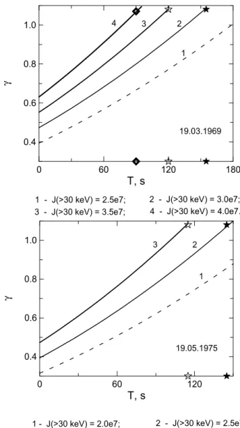
Fig. 4.Change of the temporal growth rate of whistler waves during two SC events. Planetary magnetic activity preceding the SC events is low (Kp=1+and 0). The different curves correspond to differ-ent assumptions of the initial flux of trapped electrons at energies E≥30 keV for the given values ofKp. The symbols show when the wave increment reaches the generation threshold.
the kinetic energy of trapped electrons. The change in kinetic energy per unit time during the SC is written as (Osepian, 1973; Mal’tzev, 1998):
dE dt =
5 2 −E
1
B −
dB dt .
Then taking into account betatron acceleration, the frozen-in flux condition and assumfrozen-ing that the energetic spectrum of trapped electrons withE≥30 keV is described by an expo-nential (dj/dE=j0exp(−Eres/E0) function we obtain
dlnη
dt ≈
5 2−
Then the differential equation describing the change in the wave growth rate during SC events observed against a quiet background (Kp<2) can be written in the form:
dγ dt =
3.5b 1+btγ +
1 A−
b
1+btγ . (7)
Figure 4 shows calculations of how quickly the wave growth rate increases to the wave-generation threshold at times of two real SC events which were accompanied by VLF and absorption bursts. The first case is the SC event observed at 19:58 UT on 19 March 1969 (Fig. 2a). The amplitude of SC 1B is 40 nT, T=180 s,Kp=1+. The second case is the SC
observed at 19:51 UT on 19 May 1975. Here1B=45 nT, T=150 s, Kp=0+. The different curves correspond to
dif-ferent assumptions of the initial flux of trapped electrons at energies E≥30 keV. Initial valuesγ0 are taken from
Ta-ble 2 (column 3). The symbols show when the wave growth rate reaches the generation threshold. The minimum delay time is about 90–110 s. Note that delays of 1–2 min between SC and absorption bursts can be discerned in Figs. 1a and 2a. Note also that even quite large SC amplitudes would not lead to whistler wave generation (curves 1) if the SC events occurred against a completely quiet background (Kp=0).
In Table 2, in the last column, we present the minimum magnitude of the magnetic field jump, 1B, which would causes an increase of spatial wave growth rateγ /Vg to the
threshold magnitude γt h/Vg for different pre-conditions in
the magnetosphere. To calculate these values, solutions of the differential Eq. (7) were obtained for different initial val-uesγ0corresponding to initial values of trapped flux at the
givenKp. The SC rise time is taken to be equal T=180 s.
It is seen that in the absolutely quiet magnetosphere (Kp=0)
very large SC amplitudes (1B=80−55 nT) are required to excite the whistler cyclotron instability atL=5.3. ForKp
in the range 1+ to 2-, the minimum magnitude1B needed is 25 nT. These results are quantitatively consistent with our experimental data which indicate a threshold magnitude1B about 30 nT (Fig. 3).
4 Calculation of diffusion coefficients and cosmic radio-noise absorption during SC events using the whistler cyclotron instability theory
Values of temporal γ and spatial γ /Vg growth rates
pre-sented in Table 2 show that when initial fluxes of trapped electrons J (E≥30 keV) at L=5.3 are large enough (for Kp≥2), the ambient electron distribution is unstable or
nearly unstable to whistler mode waves. A quasi-equilibrium state, where there is a balance between sources and sinks of particles and waves, may exist before the SC events, keeping the growth rate of whistler waves near or slightly above the level of marginal stability (γ ≈ν). This implies that riome-ters can measure significant background absorption preced-ing SC events, as is seen in Figs. 1b and 2b. In this case, even a small external perturbation1Bcan result in positive wave growth rate, enhancement of pitch-angle diffusion and
absorption bursts during the SC, as is seen in Figs. 1b, 2b and 3. When a quasi-equilibrium state between waves and parti-cles is present at the initial momentt0and the relaxation time TRelof the system to a new a diffusion equilibrium
configu-ration is small compared to the duconfigu-ration of the SC (TRel<T)
it is possible to evaluate the relative change in the diffusion coefficientD∗(T )/D∗(t0)caused by the SC.
In this section we apply the quasi-linear theory of whistler instability to evaluate changes in the pitch-angle diffusion co-efficientD∗at the edge of the loss cone and to calculate ab-sorption A(T) caused by a magnetic field perturbation1B. We resolve a set of three coupled differential equations de-scribing the change in anisotropy index, temporal growth rate and diffusion coefficient due to both compression and diffu-sion processes taking place during the SC.
Simple analytical expressions for anisotropy are given by the theory only for the limits of weak and strong diffusion (Kennel and Petschek, 1966; Etcheto et al., 1973). In the regime of very weak diffusion the anisotropy A− is inde-pendent of the diffusion coefficient A−=1/2ln(1/α0). In the regime of strong diffusionA−=α2o/4D∗T .For an arbi-trary diffusion strengthA−∼1/D∗βand the relation between A−andD∗can be written in the following form (Haugstad, 1975; Kirkwood and Osepian, 2001):
A−(t )=A−(t0)×(D∗(t0)/D∗(t ))β,
whereβvaries fromβ=0 toβ=1, depending on the diffusion regime assumed during the SC;D∗(t0)is an initial value of
the diffusion coefficient; preceding the SC;A−(t0)is an
ini-tial anisotropy index given by Eq. (5). Then the change in anisotropy during the SC is described by the equation:
dlnA−
dt =
(1+A−) A−
b (1+bt )−β
dlnD∗
dt . (8)
Finally, the differential Eq. (7), describing the change in the wave incrementγ in response to changes inB, ηandA−, is reduced to:
dγ dt =
3.5b 1+btγ +
1 A−
b
1+btγ −βγ 1 D∗
dD∗
dt . (9)
Since the diffusion coefficient due to whistler-particle inter-action is proportional to the square of the wave amplitude, the equation for the diffusion coefficient is written as (Coro-niti and Kennel, 1970)
dD∗
dt =2(γ (t )−γ (t0))D
∗.
(10) The coupled set of differential Eqs. (8–10) have been resolved for different values β=0−1, magnitudes 1B=5−40 nT and T=120−360 s. Calculations have been made for L-shells 5.3, 6.0 and 6.6. Figure 5 shows changes in anisotropy index A−, wave increment γ and diffusion coefficient D∗ at the equatorial plane (L=5.3) caused by a magnetic field perturbation 1B=40 nT with duration T=180 s. The initial wave growth rate γ (t0) is
anges of anisotropy index A−, wave increment γ and diffusion coefficien
0 30 60 90 120 150 180 0.20
0.24 0.28 0.32 0.36 0.40
A
-0 30 60 90 120 150 180
Time, s
1E-3 1E-2 1E-1
D*
, r
a
d
2 s
-1
β=0.0
0 30 60 90 120 150 180 1.08
1.09 1.10 1.11 1.12 1.13 1.14 1.15
γ
, s
-1
β=0.01
β=0.1
β=0.2
β=0.01 β=0.2
β=0.3
β=0.4 β=0.3
β=0.5
a
b
c
β=1.0 β=1.0 β=0.05−1.0
β=0.05
β=0.05 β=0.1
β=0.01
Fig. 5. Changes in anisotropy indexA−, wave incrementγ and diffusion coefficientD∗at the equatorial plane (L=5.3) caused by magnetic field perturbation1B=40 nT with durationT=180 s. Pa-rameterβcharacterizes diffusion strength assumed during the SC.
Kp=2. Initial values of the anisotropy index (A−(t0)=0.3)
and diffusion coefficient (D∗(t0)=8.8×10⁻⁴ rad2s−1) are
assumed to be equal to typical values of these parameters for the background equilibrium state at a given L-shell (Kirkwood and Osepian, 2001).
0.0 0.1 0.2
∆
B/B
o1 10 100 1000
D
*(T)
/ D*
o
β=0.06 : L=5.3, L=6.0, L=6.6;
β=0.6 : L=5.3,
β=0.2 : L=5.3, L=6.0, L=6.6;
L=6.0, L=6.6;
β=0.1 : L=5.3,
β=0.4 : L=5.3,
L=5.3,
L=6.0, L=6.6;
L=6.0, L=6.6;
β=1.0 : L=6.0, L=6.6
β=0.06 β=0.1
β=0.2
β=0.4
β=0.6
β=1.0
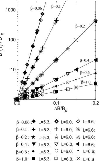
Fig. 6. Magnitude of relative change of diffusion coefficient D∗(T )/D∗(t0)as a function of1B/B0obtained for different val-ues of parameterβ.
The process of magnetic field compression leads to an un-limited increase in A−, γ andD∗. As soon as the diffu-sion process is turned on, anisotropy decreases very quickly and growth of the wave increment and diffusion coefficient is limited. The growth duration of the wave increment is less than the SC rise time. It depends on the diffusion strength (parameterβ). In the regime of weak diffusion, energy ac-cumulation by the wave lasts longer than in the regime of strong diffusion. Thus, the wave–particle system reaches a new quasi-equilibrium state in the early phase of the SC with values ofγ (t )close to but a little above the initial valueγ0.
Since the relaxation time TRel (maximum value TRel
is about 30 s) of the system to a new diffusion equilib-rium is less than the SC rise time, T, we can determine the magnitude of relative change in diffusion coefficient D∗(T )/D∗(t0)for different diffusion regimes realised
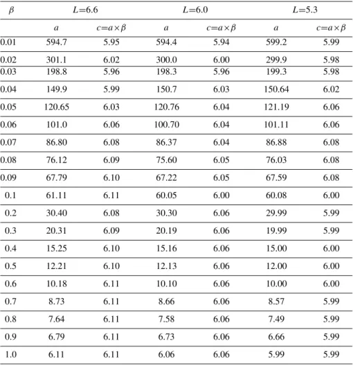
Table 3.Coefficientsaandcin Eq. (11) at the differentL-shells found as a result of numerical solution of Eqs. (8–10).
β L=6.6 L=6.0 L=5.3
a c=a×β a c=a×β a c=a×β
0.01 594.7 5.95 594.4 5.94 599.2 5.99
0.02 301.1 6.02 300.0 6.00 299.9 5.98
0.03 198.8 5.96 198.3 5.96 199.3 5.98
0.04 149.9 5.99 150.7 6.03 150.64 6.02
0.05 120.65 6.03 120.76 6.04 121.19 6.06
0.06 101.0 6.06 100.70 6.04 101.11 6.06
0.07 86.80 6.08 86.37 6.04 86.88 6.08
0.08 76.12 6.09 75.60 6.05 76.03 6.08
0.09 67.79 6.10 67.22 6.05 67.59 6.08
0.1 61.11 6.11 60.05 6.00 60.08 6.00
0.2 30.40 6.08 30.30 6.06 29.99 5.99
0.3 20.31 6.09 20.19 6.06 19.99 5.99
0.4 15.25 6.10 15.16 6.06 15.00 6.00
0.5 12.21 6.10 12.13 6.06 12.00 6.00
0.6 10.18 6.11 10.10 6.06 10.00 6.00
0.7 8.73 6.11 8.66 6.06 8.57 5.99
0.8 7.64 6.11 7.58 6.06 7.49 5.99
0.9 6.79 6.11 6.73 6.06 6.66 5.99
1.0 6.11 6.11 6.06 6.06 5.99 5.99
1B/B0at a givenL-shell and parameterβ: D∗(T )
D∗0 =exp
a1B B0
=exp c
β 1B
B0
, (11)
where the coefficientsaandc(c=a×β)have the same val-ues at anyL-shell for a givenβ. They are presented in Ta-ble 3. Solutions of Eqs. (8–10) obtained for different val-ues of the SC rise timeT show that the maximum change in diffusion coefficientD∗(T )is by a factor 1.2 for the range T=120−360 s.
Provided that the wave-particle system is in a quasi-equilibrium state, the total flux of precipitating electronsJp
withE≥EResis proportional to the diffusion coefficient and
at the time of the SC events we have Jp(T )=Jp(t0)exp
c β
1B B0
.
Knowing the magnitude of the field perturbation1Bin the equatorial magnetosphere at the givenL-shell and recalling that absorptionAis proportional toJp(E≥ERes)−, we are
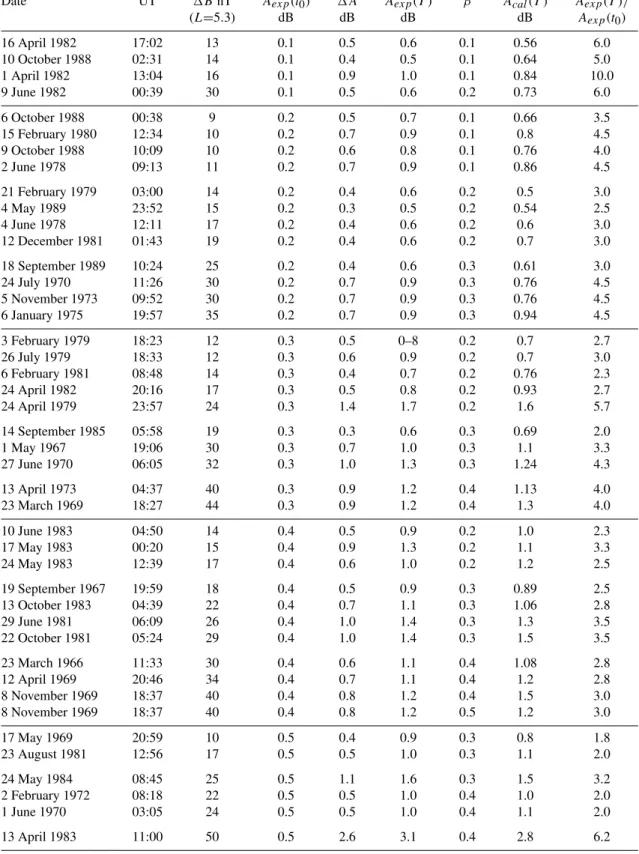
able to calculate absorption SCA for real SC events for dif-ferent diffusion regimes. In Table 4 we compare calculated
values of absorptionAcalwithAexpmeasured in Loparskaya
to evaluate the ability of the quasi-linear model to describe a number of qualitative and quantitative features of absorption bursts induced by SCs, and to determine the diffusion regime realized during the real SC events. Note that, although all available events have been analysed, we include only a se-lection of typical examples in Table 4 covering the range of values of1BandAexprepresented in the full data set.
5 Discussion and Conclusions
We have examined bursts of cosmic noise absorption (SCA) observed during sudden commencements (SC) of geomag-netic storms. We find that the response of cosmic noise ab-sorption to the passage of an interplanetary shock depends on the level of planetary magnetic activity preceding the SC and on the magnitude of the geomagnetic field perturbation 1induced by the SC at the givenL-shell in the equatorial magnetosphere. We have shown that, for SC-events observed against a quiet background (Kp<2), an effect of the SC on
wind shock exceeds a critical value1Bt h. In contrast, SC
events observed against an active background (Kp>2) are
accompanied by impulsive absorption bursts, however small the perturbation1B.
Using a simple quasi-linear model we show that proper-ties of absorption bursts, such as the dependence of their oc-currence onKp-index, the time delay between SC and
ab-sorption bursts and the existence of a threshold SC ampli-tude1Bth, can be explained and quantitatively predicted by
the whistler cyclotron instability theory. We have investi-gated changes in the whistler growth rate during typical SC taking into account changes in all parameters in the rele-vant equation, including changes in the fraction of resonant electrons. Changes in the latter parameter are mainly due to acceleration of trapped electrons in the induction electric field. Note that an increased flux of trapped electrons with E>30 keV, consistent with the betatron acceleration effect, was observed by a geosynchronous satellite during the SC event on 22 March 1979 (Wilken et al., 1986). Changes in plasma density due to the frozen-in flux condition are also taken into account.
We show that the existence of a threshold value1Bt h
de-duced from experimental data, can be related to the exis-tence of a threshold for exciting and maintaining the whistler cyclotron instability which is predicted by the quasi-linear theory. We find that in the quiet magnetosphere the mini-mum jump1B of magnetic field which increases the wave growth rate to the generation threshold atL=5.3 is close to the experimental magnitude1Bt hof about 30 nT. It is clear
that the minimum magnitude1Bt hdepends on pre-history,
i.e. on the state of the magnetosphere, at a given L-shell before the SC event, in particular on the characteristics of the magnetospheric plasma (cold and hot plasma density and pitch-angle distribution function of the resonant electrons). This means that the threshold magnitude 1Bt h should
de-pend on theL-shell and MLT sector. In the afternoon sec-tor, at 14:00–18:00 MLT, where initial trapped fluxes are the lowest, the minimum jump1Bt h, deduced from our
calcula-tions is about 40 nT, whereas in the morning sector it is about 25–30 nT. Note that Ortner et al. (1962) and Hartz (1963) re-ported local time and latitude dependences of SCA bursts, with the highest probability that they should be observed in the morning-noon sector at geomagnetic latitudes 64◦−66◦.
We have also investigated changes in anisotropy, wave growth rate and diffusion coefficient during the early phase of the SC, during the SC rise time, for different assumed diffu-sion regimes. We have found that when the diffudiffu-sion process is turned on, the wave growth saturates very quickly. The maximum growth duration is 30–15 s in the regime of weak diffusion and 3–1 s for moderate – strong diffusion, whereas the typical SC rise time is 120–180 s. Saturation corresponds to the onset of nonlinear processes within the wave-particle system. In conditions of weak diffusion the system relaxes to a new equilibrium state with a higher level of wave en-ergy than in conditions of strong diffusion. As a result, the same perturbation1Bhas the greatest effect on the diffusion coefficient when conditions of weak diffusion prevail.
Analytical expressions describing the dependence of the diffusion coefficient and resultant absorption on the value of the magnetic field perturbation1B, induced by the SC and on the strength of the diffusion process (β), have been de-duced. Results are presented in Table 4. This shows that the model can describe both the magnitude of observed absorp-tion bursts(Aexp(T ))and the dependence of the absorption
increase (Aexp(T )/Aexp(t0)) on the SC amplitude1B and
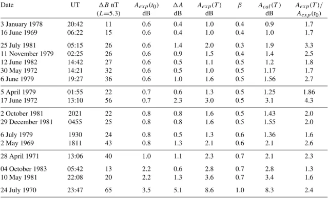
parameterβ. Here it should be noted that the observed val-ues of absorption correspond to a regime of weak-moderate diffusion. Moreover, the values ofβ, which have to be as-sumed to satisfy the experimental data, are found to depend on the diffusion regime existing before the SC event. If the SC occurs against a background of weak diffusion (initial precipitation is small, A0=0.1−0.3dB), only a weak
dif-fusion regime is realized during SC events (β=0.1−0.3). When the background absorption is higher, moderate diffu-sion (β=0.4−0.6) is needed to explain the observed SCA amplitudes. Only in rare cases, when we observe strong ab-sorption before the SC and large values of1B, does the dif-fusion during the SC become close to strong (β=0.7−1.0).
Further, it can be noted that the largest relative changes in measured absorption, (Aexp(T )/Aexp(t0)), take place when
the pitch angle diffusion is weak. For example, for1Babout 26 nT values of relative absorption increases of 3.3, 2.5, 2.0 and 1.6 correspond toβ=0.3,0.4,0.5 and 0.6, respectively. As the theory predicts (Fig. 5 and Eq. (11)), in the regime of weak diffusion, the value of wave growth rateγ (t )in a new equilibrium state is higher, and changes in diffusion coeffi-cient are larger than in the regime of strong diffusion.
6 Summary
Bursts of cosmic noise absorption induced by a sharp jump in the magnetic field (1B) in the equatorial plane of the mag-netosphere have been studied on the basis of a large experi-mental data set (about 300 events). We have shown that, for events preceded by quiet conditions, a threshold value1Bt h
exists below which the magnetic field perturbation does not cause a detectable absorption change. For events preceded by more active conditions the effect in absorption is observed regardless of the level of magnetic perturbation. The results are explained quantitatively in the framework of whistler cy-clotron instability theory. We have shown that the minimum magnitude 1Bt h needed for exciting and maintaining the
whistler cyclotron instability depends on pre-history, i.e. on the state of the magnetosphere at a givenL-shell before the SC event, in particular on the characteristics of the magne-tospheric plasma. Also, it should depend on theL-shell and MLT sector.
Table 4. Comparison of observed and calculated cosmic-noise absorption changes for a representative subset of the events analysed. Ob-served quantities are dates, times (UT), magnitudes of the SC magnetic field jump (1B), the absorption preceeding the SC (Aexp(t0)), the absorption increase associated with the SC (1A) and the total abrorption following the SC (Aexp(T )).βis the diffusion strength parameter which is found to be necessary to fit the observedAexp(T )(from the range represented in Table 3). Acal(T )are the calculated absorption andAexp(T )/Aexp(t0)) the relative absorption increase.
Date UT 1BnT Aexp(t0) 1A Aexp(T ) β Acal(T ) Aexp(T )/
(L=5.3) dB dB dB dB Aexp(t0)
16 April 1982 17:02 13 0.1 0.5 0.6 0.1 0.56 6.0
10 October 1988 02:31 14 0.1 0.4 0.5 0.1 0.64 5.0
1 April 1982 13:04 16 0.1 0.9 1.0 0.1 0.84 10.0
9 June 1982 00:39 30 0.1 0.5 0.6 0.2 0.73 6.0
6 October 1988 00:38 9 0.2 0.5 0.7 0.1 0.66 3.5
15 February 1980 12:34 10 0.2 0.7 0.9 0.1 0.8 4.5
9 October 1988 10:09 10 0.2 0.6 0.8 0.1 0.76 4.0
2 June 1978 09:13 11 0.2 0.7 0.9 0.1 0.86 4.5
21 February 1979 03:00 14 0.2 0.4 0.6 0.2 0.5 3.0
4 May 1989 23:52 15 0.2 0.3 0.5 0.2 0.54 2.5
4 June 1978 12:11 17 0.2 0.4 0.6 0.2 0.6 3.0
12 December 1981 01:43 19 0.2 0.4 0.6 0.2 0.7 3.0
18 September 1989 10:24 25 0.2 0.4 0.6 0.3 0.61 3.0
24 July 1970 11:26 30 0.2 0.7 0.9 0.3 0.76 4.5
5 November 1973 09:52 30 0.2 0.7 0.9 0.3 0.76 4.5
6 January 1975 19:57 35 0.2 0.7 0.9 0.3 0.94 4.5
3 February 1979 18:23 12 0.3 0.5 0–8 0.2 0.7 2.7
26 July 1979 18:33 12 0.3 0.6 0.9 0.2 0.7 3.0
6 February 1981 08:48 14 0.3 0.4 0.7 0.2 0.76 2.3
24 April 1982 20:16 17 0.3 0.5 0.8 0.2 0.93 2.7
24 April 1979 23:57 24 0.3 1.4 1.7 0.2 1.6 5.7
14 September 1985 05:58 19 0.3 0.3 0.6 0.3 0.69 2.0
1 May 1967 19:06 30 0.3 0.7 1.0 0.3 1.1 3.3
27 June 1970 06:05 32 0.3 1.0 1.3 0.3 1.24 4.3
13 April 1973 04:37 40 0.3 0.9 1.2 0.4 1.13 4.0
23 March 1969 18:27 44 0.3 0.9 1.2 0.4 1.3 4.0
10 June 1983 04:50 14 0.4 0.5 0.9 0.2 1.0 2.3
17 May 1983 00:20 15 0.4 0.9 1.3 0.2 1.1 3.3
24 May 1983 12:39 17 0.4 0.6 1.0 0.2 1.2 2.5
19 September 1967 19:59 18 0.4 0.5 0.9 0.3 0.89 2.5
13 October 1983 04:39 22 0.4 0.7 1.1 0.3 1.06 2.8
29 June 1981 06:09 26 0.4 1.0 1.4 0.3 1.3 3.5
22 October 1981 05:24 29 0.4 1.0 1.4 0.3 1.5 3.5
23 March 1966 11:33 30 0.4 0.6 1.1 0.4 1.08 2.8
12 April 1969 20:46 34 0.4 0.7 1.1 0.4 1.2 2.8
8 November 1969 18:37 40 0.4 0.8 1.2 0.4 1.5 3.0
8 November 1969 18:37 40 0.4 0.8 1.2 0.5 1.2 3.0
17 May 1969 20:59 10 0.5 0.4 0.9 0.3 0.8 1.8
23 August 1981 12:56 17 0.5 0.5 1.0 0.3 1.1 2.0
24 May 1984 08:45 25 0.5 1.1 1.6 0.3 1.5 3.2
2 February 1972 08:18 22 0.5 0.5 1.0 0.4 1.0 2.0
1 June 1970 03:05 24 0.5 0.5 1.0 0.4 1.1 2.0
Table 4.Continued.
Date UT 1BnT Aexp(t0) 1A Aexp(T ) β Acal(T ) Aexp(T )/
(L=5.3) dB dB dB dB Aexp(t0)
3 January 1978 20:42 11 0.6 0.4 1.0 0.4 0.9 1.7
16 June 1969 06:22 15 0.6 0.4 1.0 0.4 1.0 1.7
25 July 1981 05:15 26 0.6 1.4 2.0 0.3 1.9 3.3
11 November 1979 02:25 26 0.6 0.9 1.5 0.4 1.4 2.5
12 June 1982 14:42 27 0.6 0.5 1.1 0.5 1.2 1.8
30 May 1972 14:21 32 0.6 0.5 1.0 0.5 1.17 1.7
6 June 1979 19:27 36 0.6 1.0 1.6 0.5 1.56 2.7
5 April 1979 01:55 22 0.7 0.6 1.3 0.5 1.25 1.86
17 June 1972 13:10 56 0.7 2.3 3.0 0.5 3.1 4.3
2 October 1981 2021 22 0.8 0.8 1.6 0.5 1.43 2.0
29 December 1981 0455 25 0.8 0.8 1.6 0.5 1.55 2.0
6 July 1979 1930 24 0.8 0.5 1.3 0.6 1.36 1.6
2 May 1969 1811 43 0.8 1.3 2.1 0.6 2.1 2.6
28 April 1971 13:06 40 1.0 1.1 2.3 0.7 2.1 2.3
04 October 1983 05:42 13 2.2 0.6 2.8 0.7 2.8 1.3
10 May 1981 22:08 20 2.2 1.3 3.6 0.7 3.4 1.6
24 July 1970 23:47 65 3.5 5.1 8.6 1.0 8.3 2.4
of observed absorption bursts and the dependence of the ab-sorption increase on1Band a parameterβ. For a given1B, the values ofβ, which satisfy the experimental data, depend on the diffusion regime existing before the SC event. As can be seen in Table 4, weak to moderate diffusion regimes are realized during most of the SC events (β=0.1−0.6).
Thus, we find that the quasi-linear whistler-cyclotron in-stability model is well able to explain both qualitative and quantitative features of cosmic-noise absorption bursts asso-ciated with sudden commencements of geomagnetic storms.
Appendix A
Calculation of SC-amplitude in the magnetosphere
We determine the value of the perturbation1Bin magnetic field strength, in the equatorial magnetosphere at theL-shell corresponding to the riometer station Loparskaya (L=5.3) using both the amplitude,1H, measured at the Earth’s sur-face and information on the variation of solar wind parame-ters at the front of the bow shock obtained from the satellites IMP-8 and WIND.
It is known that a sharp increase in dynamic pressure,Pd,
of the solar wind on the magnetosphere acts to compress the magnetosphere. This effect is displayed in variations of the magnetic field inside the magnetosphere, both at satel-lite altitudes and at the Earth’s surface. Such impulses seen at the Earth’s surface have long been identified as “sudden impulses” or “sudden commencements” when followed by a geomagnetic storm. The physical reason for the effect is an increase in the Chapman-Ferraro currents. At the Earth’s
sur-face, at stations located near equator, the effect of the shock is seen as a sharp increase,1H, of the horizontal component of geomagnetic field. To evaluate1B we apply the follow-ing formulae obtained in accordance with Mead (1964) and Siscoe (1966):
1B=BCF I −BCF P =BCF P{(PS2/PSI)1/2−1} (A1a) 1B= 2
3 BCF P BCF P E
1H
cosϕ, (A1b)
wherePS1,PS2are the dynamic pressure of the solar wind
before the shock wave passes and at the front of the shock wave or discontinuity, respectively. (PS=kρVSW2 ,ρ≡mpnp,
whereρis the density of the solar wind;VSWis the velocity
of the solar wind;k∼=1);BCF P E andBCF P are the
horizon-tal components of the magnetic field due to the Chapman-Ferraro currents at the plane of the geomagnetic equator at the Earth’s surface and at distance r (in Earth radii) in the magnetosphere for conditions corresponding to the quiet so-lar wind,BCF I is the value of the field due to the
Chapman-Ferraro currents at the same place as BCF P but during the
disturbance; 1H is the amplitude of the SC at the Earth’s surface at latitudeϕ.
The values of the SC-amplitude atL=5.3 (Table 1) ob-tained with Eq. (A1a), on the basis of measurements of the solar wind parameters by IMP-8, and Eq. (1b) using1H val-ues measured at the station Alibag (ϕ=18.6◦N,λ=72.9◦E; 8‘=12.4◦N,3=142.9◦E) are in good agreement. Magnetic fields of the Chapman-Ferraro currents,BCF P E andBCF P,
Acknowledgements. Topical Editor T. Pulkkinen thanks S. Sam-sonov and another referee for their help in evaluating this paper.
References
Binsak, J. H.: Plasmapause observations with MLT experiment on Imp-2., J.Geophys. Res., 72, No. 21, 5231–5237, 1967. Brown, R. R., Hartz, T. R., Landmark, B., Leinbach, T., and Ortner,
J.: Large-scale electron bombardment at the atmosphere at the sudden commencement of geomagnetic storm., J. Geophys. Res., 66, 1035, 1961.
Carpenter, D. L.: Relations between the dawn minimum in the equa-torial radius of the plasmapause andDst,Kpand localKat Byrd station., J. Geophys. Res., 72, No. 11, 2969–2971, 1967; Carpenter, D. L., Chappel, C. R.: Satellite studies of
magneto-spheric substorm on August 15, 1968., J. Geophys. Res., 78, No. 16, 3602–3607, 1973.
Chappel, C. R., Harris, K. K., Sharp, G. W.: A study of the influence of nagnetic activity of the local of the plasmapause as measured by Ogo-5, J. Geophys. Res., 75, No.1, 50–56, 1970a.
Chappel C. R., Harris, K. K., Sharp, G. W.: The morphology of the bulge region of the plasmasphere, J. Geophys. Res., 75, No. 19, 3848–3861, 1970b.
Chappel, C. R., Harris, K. K., and Sharp, G .W.: The dayside of the plasmasphere, J. Geophys. Res. 76, 7632–7647, 1971.
Collis, P. N., Hargreaves, J. K., Korth, A.: Loss cone fluxes and pitch angle diffusion at the equatorial plane during auroral radio absorption events,, Planet. Space Sci., 45, No. 4, 231–245, 1983. Coroniti, V. F. and Kennel, C. F.: Electron Precipitation Pulsations,
J. Geophys. Res., 75, 7, 1279–1289, 1970.
Cornilleau-Wehrlin, N., Solomon, J., Korth, A., and Kremser, G.: Experimental study ofthe relationship between energetic elec-trons and ELF waves observed on board GEOS: A support to quasi-linear theory, J. Geophys. Res., 90, No. A5, 4141–4154, 1985.
Davidson, G. T. and Chiu, Y. T.: A closed nonlinear model of wave-particle interactions in the outer trapping and morningside auro-ral regions, J. Geoph. Res., 91, A12, 13 705–13 710, 1986. Davidson, G. T., Filbert, P., Nightingale, C. R. W., Imhof, W. L.,
Reagon, J. B., and Whipple, E. C.: Observations of intense trapped electron fluxes at synchronous altitudes. J. Geophys. Res., 93, A1, 77–95, 1988.
Demekhov, A. G., and Trakhtengerts, V. Y.: A mechanism of for-mation of pulsating aurorae, J. Geophys. Res., 99, A4, 5831– 5841,1994.
Demekhov A. G., Lyucbhich, A. A., Trakhtengerts, V. Y., Titova, E. E., Manninen, J., and Turunen, T.: Modeling of nonstationary electron precipitation by the whistler cyclotron instability, Ann. Geophys., 16, 1455–1460, 1998.
Erlandson R. E., Sibeck, D. G., Lopez, R. E., Zanetti, L. J., and Potemra, T. A.: Observations of solar wind pressure initiated fast mode waves at the geostationary orbit and in polar cap, J. Atmos. Terr. Phys., 53, 231–239, 1991.
Etcheto J., Gendrin, R., Solomon, J., and Roux, A.: A self-consistent theory of magnetospheric ELF hiss, J. Geophys. Res., 78, 34, 8150–8165,1973.
Gail, W. B., Inan, U. S., Helliwell, R. A., Carpenter, D. L., Kris-naswarny, S., Rosenberg, T. J., and Lanzerotti, L. J.: Character-istics of wave-particles interactions during sudden commence-ments, 1.Ground-based observations, J. Geophys. Res., 95, A1, 119–137, 1990.
Gail, W. B. and Inan, U. S.: Characteristics of wave-particles inter-actions during sudden commencements, 2. Spacecraft observa-tions, J. Geophys. Res., 95, A1, 139–147, 1990.
Harris, K. K., Sharp, G. W., and Chappel, C. R.: Observation of the plasmapause from OGO-5, J.Geophys. Res., 75, No. 1, 219–224, 1970.
Hartz, T. R.: Multistation riometer observations in Radio As-tronomical and Satellite Studies of the Atmosphere, edited by Aarons, J., North Holland, Amsterdam, 220–237, 1963. Haugstad, B. C.: Modification of the theory of electron precipitation
pulsations., J. Atmosp. Terr. Phys., 37, 257–272, 1975.
Hayashi, K., Kokubun, S., and Oguti, T.: Polar chorus emission and worldwide geomagnetic variation, Rep. Ionos. Space Res. Jpn., 22, 149, 1968.
Kennel, C. F. and Petschek, H. E.: Limit of stably trapped particle fluxes, J. Geophys. Res., 71, 1, 1–28, 1966.
Kirkwood, S. and Osepian, A.: Pitch-angle diffusion coefficients and precipitating electron fluxes inferred from EISCAT radar measurements at auroral latitudes, J. Geophys. Res., 106, A4, 5565–5578, 2001.
Kivelson, M. G., Farley, T. A., and Aubry, M. P.: Satellite studies of magnetospheric substorm on August 15, 1968, 5. Energetic elec-trons, spatial boundaries and wave-particle interactions at OGO 5., J. Geophys. Res., 78,16, 3079–3092, 1973.
Kleimenova, N. G. and Osepian, A. P.: VLF emissions at the time of sudden commencements (in Russian), Geomagn. and Aeronomy, XXII, No. 4, 681–683, 1982.
Kokubun S.: Characteristics of storm sudden commenecement at geostationary orbit., J. Geophys. Res., 88, 10 025, 1983. Laakso, H. and Schmidt, R.: Pc4-5 pulsations in the electric field at
geostationary orbit (GEOS 2) triggered by suddern storm com-mencements, J. Geophys. Res., 94, A6, 6626–6632, 1989. Lyons, L. R., Williams, D. J.: The quiet time structure of energetic
(35–560 keV) radiation belt electrons., J. Geophys. Res., 80, 7, 943–949, 1975.
Mal’tsev, Yu. P.: Electric field induced in the magnetosphere by sudden impulse, Geomagn. and Aeronom., v. 1, 23–26, 1998. Manninen J., Turunen, T., Lubchich, A., Titova, E., and Yahnina, T.:
Relations of VLF emissions to impulsive electron precipitation measured by EISCAT radar in the morning sector of auroral oval, J. Atmos. and Terr. Phys., 58, No. 1–4, 97–106, 1996.
Mead, G. D.: Deformation of the geomagnetic field by the solar wind., J. Geophys. Res., 69, 7, 1181–1195, 1964.
Morgan, M. G. and Maynard, N. C.: Evidence of dayside plasma-spheric structure through comparisions of ground-based whistler data and Explorer-45 plasmapause data, J. Geophys. Res., 81, 22, 3922–3928, 1976.
Morozumi, H. M.: Enhancement of VLF chorus and ULF at the time of SC., Rep. Ionos. Space Res. Jpn., 19, 371, 1965. Nopper R.W., Jr., Hugher W. J., Maclennan C. G. and McPherron R.
L., Impulsive-excited pulsations during the July 29, 1977, event. J. Geophys. Res., 87, No. A8, 5911-5916, 1982.
Ortner, J. B., Hultqvist, B., Brown, R. R., Hartz, T. R., Holt, O., Landmark, B., Hook, J. L., and Leinbach, H.: Cosmic noise ab-sorption accompanying geomagnetic storm sudden commence-ment, J. Geophys. Res., 67, 4169, 1962.
Osepian A.: Betatron acceleration at the time of SC events. Inves-tigations of geomagnetism and aeronomy in the auroral zone (in Russian), Science, 186–193, 1973.
Perona, G. E.: Theory on the precipitation of magnetospheric elec-trons at the time of sudden commencements, J. Geophys. Res., 77, 101–111, 1972.
Potemra, T. A., L¨uhr, H, Zanetti, L. J., Takahashi, K., Erlandson, R. E., Marklund, G. T., Block, L. P., Blomberg, L. G., and Lepping, P. P., Multi-satellite and ground-based observations of transient ULF wave, J. Geophys. Res., 94, A3, 2543–2554, 1989. Reeves, G. D.: Energetic particle observations at geosynchronous
orbit, Proceeding of the International Workshop on Magneic Storms, edited by Kamide, Y., Sol. Terr. Environ., Nagoya, Japan, 1994.
Rycroft, M. J. and Thomas, J. O.: The magnetospheric plasmapause and the electron density through at the Alouette II orbit., Planet. Space Sci., 18, 1, 65–80, 1970.
Singh, N., Horwitz, J. L.: Plasmasphere refilling: Recent observa-tions and modeling., J. Geophys. Res., 97, No. A2, 1049–1079, 1992.
Siscoe, G. L.: A unified treatment of magnetospheric dinamics with applications to magnetic storms., Planet. Space Sci., 1966, v. 14, 10, 947–963, 1966.
Schulz M. and Davidson, G.: Limiting energy spectrum of a satu-rated radiation belt., J. Geophys. Res., 93, 1, 59–76, 1988.
Thorolfsson A., Cerisier, J. C., and Pinnock, M.: Flow transients in the postnoon ionosphere: The role of solar wind dynamic pres-sure, J. Geophys. Res., 106, A2, 1887–1901, 2001.
Trakhtengerts, V. Y., Tagirov, V. R., and Chernouss, S. A.: A cir-culating cyclotron maser and pulsed VLF emissions, Geomagn. and Aeronom., 26, 77–82, 1986.
West Jr., H. I., Buck, R. M., and Walton, J. R.: Electron pitch angle distribution throughout the magnetosphere as observed on OGO 5., J. Geophys. Res., 78, 7, 1064–1081, 1973.
Wilken, B., Baker, D. N., Higbie, P. R., Fritz, T. A., Olson, W. P., and Pfitzer, K. A.: The SSC on July 29, 1977 and its propagation within the magnetosphere, J. Geophys. Res., 87, No. A8, 5901– 5910, 1982.
Wilken, B., Baker, D. N., Higbie, P. R., Fritz, T. A., Olson, W. P., and Pfitzer K. A.: Magnetospheric configuration and energetic particle effects associated with SSC: A case study of the CDAW 6 event on March 22, 1979, J. Geophys. Res., 91, No. A2, 1459– 1473, 1986.