SRef-ID: 1432-0576/ag/2004-22-877 © European Geosciences Union 2004
Annales
Geophysicae
The statistical dependence of auroral absorption on geomagnetic
and solar wind parameters
A. J. Kavanagh1,2, M. J. Kosch3,4, F. Honary3, A. Senior3, S. R. Marple3, E. E. Woodfield1, and I. W. McCrea5
1High Altitude Observatory, NCAR, PO Box 3000, Boulder, Co., 80307-3000, USA
2formerly at: the Department of Communications Systems, Lancaster University, Lancaster, UK, and the EISCAT Group,
Space Science and Technology Dept., Rutherford Appleton Laboratory, Chilton, Didcot, UK
3Department of Communications Systems, Lancaster University, Lancaster, UK 4Honorary Reseach Fellow, University of Natal, Durban 4041, South Africa
5EISCAT Group, Space Science and Technology Dept., Rutherford Appleton Laboratory, Chilton, Didcot, Oxfordshire, UK
Received: 18 February 2003 – Revised: 31 July 2003 – Accepted: 5 August 2003 – Published: 19 March 2004
Abstract. Data from the Imaging Riometer for Ionospheric Studies (IRIS) at Kilpisj¨arvi, Finland, have been compiled to form statistics of auroral absorption based on seven years of observations. In a previous study a linear relationship be-tween the logarithm of the absorption and theKpindex pro-vided a link between the observations of precipitation with the level of geomagnetic activity. A better fit to the absorp-tion data is found in the form of a quadratic inKp for eight magnetic local time sectors. Past statistical investigations of absorption have hinted at the possibility of using the solar wind velocity as a proxy for the auroral absorption, although the lack of available satellite data made such an investigation difficult. Here we employ data from the solar wind monitors, WIND and ACE, and derive a linear relationship between the solar wind velocity and the cosmic noise absorption at IRIS for the same eight magnetic local time sectors. As far as the authors are aware this is the first time that in situ measure-ments of the solar wind velocity have been used to create a di-rect link with absorption on a statistical basis. The results are promising although, it is clear that some other factor is neces-sary in providing reliable absorption predictions. Due to the substorm related nature of auroral absorption, this is likely formed by the recent time history of the geomagnetic activ-ity, or by some other indicator of the energy stored within the magnetotail. For example, a dependence on the southward IMF (interplanetary magnetic field) is demonstrated with ab-sorption increasing with successive decreases inBz; a north-ward IMF appears to have little effect and neither does the eastward component,By.
Key words. Magnetospheric physics (energetic particles, precipitating; solar wind-magnetosphere interactions) – Ionosphere (modeling and forecasting)
Correspondence to:A. J. Kavanagh ([email protected])
1 Introduction
Understanding the variation of High Frequency (HF) radio absorption in the auroral zone is of great importance for de-termining HF radio propagation conditions. Linking the ab-sorption to parameters measured in real time, such as the solar wind velocity or interplanetary magnetic field (IMF) orientation, can lead to improved prediction models. Many workers have performed statistical studies of riometer ab-sorption in the past (e.g. Holt et al., 1961; Hartz et al., 1963; Driatsky, 1966; Hargreaves and Cowley, 1967) and the re-sults tend to confirm a diurnal variation in the absorption pattern. Differences have arisen depending on the method of compiling the statistics (Hargreaves, 1969); by sampling absorption at regular intervals a maximum in the morning sector is emphasized, whereas through identification of dis-crete events a peak before magnetic midnight is highlighted. Absorption sampled at too low a frequency will also de-emphasise the midnight peak. Similarly, different parameters have been chosen to reproduce the morphology of the ab-sorption oval; these include the mean and median of the dis-tributions and the occurrence of absorption above a threshold level (e.g. 1 dB at a given riometer frequency) (Hargreaves, 1966; Hargreaves and Cowley, 1967; Foppiano and Bradley, 1985).
Identification of the occurrence of absorption has led to the development of prediction models (e.g. Foppiano and Bradley, 1983 and 1984) that depend both on MLT (magnetic local time) and the level of geomagnetic activity. Hargreaves (1966) examined quantitive relationships between observed absorption and theKpandApgeomagnetic indices, and used the limited available data to link the energy deposition to the solar wind speed. This highlighted the dependence of ab-sorption on the solar wind speed, demonstrating an important effect in the coupling of interplanetary space phenomena to the ionosphere.
10o
E
15o
E 20oE 25oE
30oE
66o
N 67o
N 68o
N 69o
N 70o
N 71o
N
1 7
43 49
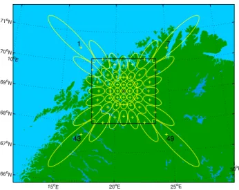
Fig. 1.Beam projection of IRIS at 90 km altitude. The contours
de-fine the−3 dB points and the black square shows the calculated field
of view used in the IRIS images. The four corner beams are marked with their corresponding identification numbers, and the black cross marks the centre beam (25) which is used in this study. The large circle centred on the cross shows the contour of the co-located wide beam.
Composition Explorer) spacecraft situated at the L1 point. An upstream vantage point such as this results in early warn-ings of possible conditions at Earth from ten minutes to over an hour before, depending on the solar wind speed. In this study we use the in situ solar wind observations to consider the link between cosmic noise absorption (CNA) and vari-ations in the solar wind velocity and IMF orientation. The dependence of CNA onKp is investigated with a new data set of seven years worth of narrow beam riometer observa-tions. An improvement over previous relationships is found, although the variation of absorption within a three-hour inter-val limits the use of such a relationship. As far as the authors are aware, for the first time direct satellite measurements are used to determine an empirical relationship between the ab-sorption and solar wind velocity. There is also a an unex-pected general increase in CNA during southward IMF con-ditions.
2 Instrumentation
The Imaging Riometer for Ionospheric Studies (IRIS) at Kilpisj¨arvi, Finland (69.05◦N, 20.79◦E), began operations in September 1994, (Browne et al., 1995), based on a con-cept introduced by the University of Maryland (Detrick and Rosenberg, 1990) of using a single phased array to generate imaging beams. Consisting of an array of 64 dipoles, the in-strument produces 49 beams at various angles to the zenith (Fig. 1), as well as a single wide beam. Beam widths in the D-layer are of the order of 20 km wide near the zenith, be-coming progressively wider with decreasing elevation angle. All of the beams are sampled every second, although in the
following study the data are at averages greater than or equal to 10 min.
For this study the zenithal beam has been used to provide data; the centre of this beam lies at 66.06◦magnetic latitude and 104.32◦magnetic longitude (altitude adjusted corrected geomagnetic coordinate system (Baker and Wing, 1989)) in a plane at 90 km altitude. The position has been calculated for 1998 using the IGRF-2000 (International Geomagnetic Reference Field) model. Data from the zenithal beam of the imaging riometer has an advantage over wide beam riome-ters in that the integrated absorption is from a significantly smaller portion of the sky (compare 12.6◦beam width with >60◦) and thus giving a truer measure of the vertical absorp-tion.
Data from both the ACE (1998–2001) (McComas et al., 1998; Smith et al., 1998) and WIND (1995–1998) (Lep-ping et al., 1995; Ogilivie et al., 1995) spacecraft have been used to provide measurements of the solar wind and inter-planetary magnetic field. ACE was positioned at the first Lagrangian point (L1), whereas WIND was performing a more complicated orbit. A simple method of dividing the bowshock-spacecraft distance (in the GSMX-direction) by the solar wind velocity to determine the delay time to the ionosphere has been employed due to the large quantity of data. From the bowshock (considered to be at 15RE) a fur-ther 5 min is added to account for the propagation time to the magnetopause and transmission into the magnetosphere. Occasions when high-speed streams overlap with slower so-lar wind have been removed from the data set rather than attempting to compute the complicated interactions.
3 Observations
IRIS data have been taken from the epoch 1995 to 2001 in-clusive, providing a maximum of 2557 days with 144 data points (10-min. averages) in each. In practice data is lost due to maintenance time and hardware failures, accounting for less than 1% of the epoch. The most significant loss of data is due to contamination from solar radio emission (SRE) at 38.2 MHz; this increases the received signal in the riometer above the cosmic radio noise level. The absorption is calcu-lated by subtracting the received power from the quiet day curve (QDC), representing the received cosmic noise power on a day when there are no contributions to absorption from particle precipitation. A percentile method (Browne et al., 1995) is used based on a minimum of 14 days of data to gen-erate QDC for IRIS, though this has been refined to work at higher resolutions and to remove the effects of SRE from the QDC. For periods when the received power is boosted above the quiet day level negative absorption values are cal-culated which are unrealistic. To combat the effects of this phenomenon data have been removed when absorption is <−0.2 dB in any beam; a level of−0.2 dB is implemented
to account for uncertainties in the quiet day curves.
00 04 08 12 16 20 00 0
0.05 0.1 0.15 0.2 0.25 0.3 0.35 0.4
Absorption (dB @ 38.2 MHz)
MLT (h)
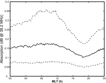
Fig. 2.Variation of median absorption in the zenithal beam of IRIS
(epoch 1995–2001). Note the diurnal variation with the morning maximum followed by a minimum close to dusk. The two dashed lines indicate the upper and lower quartiles of the distributions be-hind each time point; the interquartile range is much larger at the maximum than the minimum.
dashed lines represent the upper and lower quartiles of the distributions. A distinct diurnal variation is immediately ap-parent with a peak in the pre-noon sector (09:00–10:00 MLT) and a deep minimum in the afternoon, close to dusk. The in-terquartile range is significantly higher at the maximum, with an increase in the upper quartile, indicative of a larger occur-rence of higher absorption.
The values depicted in Fig. 2 represent the whole span of data; however, we are interested in understanding how that diurnal variation changes with geomagnetic activity. By con-sidering the distribution of absorption at each level ofKp, in-formation on the dependence of absorption on geomagnetic activity can be discerned. Figure 3 is composed of eight im-ages displaying absorption againstKpfor each local time in-terval. Occurrence is colour coded as a percentage of the total number of points in each time sector, with red being the high-est (4.5%) and black indicating zero; percentages are plotted to 0.1% accuracy. The white lines show the mean of the dis-tribution across theKpbins in each time sector. Absorption has been sorted into 0.1 dB bins and the data are plotted from 0.1 to 2 dB, since all absorption higher than this falls well below the 0.1% occurrence level. In every case the highest percentage is at the lowKpvalues and close to 0 dB; negative values make up less than 4% of the total number of points at each local time. The 00:00–03:00 MLT plot indicates a tilt in the data to higher absorption at higherKp, but the absorption is lower than 0.7 dB. By 03:00–06:00 MLT the absorption has extended to 1 dB at the top end of theKp range, though the majority of absorption is within 0 to 0.4 dB. Absorption lev-els continue to increase until 09:00–12:00 MLT, when a max-imum of 1.7 dB at the 0.1% level is recorded. This occurs at Kp=5−, and the spread ofKp values at 0.5 dB has also
in-Occurence (%)
0 2 4
0 0.5 1 1.5 2 0
2 4 6 8
00−03 MLT
Kp
0 0.5 1 1.5 2 0
2 4 6 8
03−06 MLT
0 0.5 1 1.5 2 0
2 4 6 8
06−09 MLT
Kp
0 0.5 1 1.5 2 0
2 4 6 8
09−12 MLT
0 0.5 1 1.5 2 0
2 4 6 8
12−15 MLT
Kp
0 0.5 1 1.5 2 0
2 4 6 8
15−18 MLT
0 0.5 1 1.5 2 0
2 4 6 8
18−21 MLT
Kp
0 0.5 1 1.5 2 0
2 4 6 8
21−24 MLT
Absorption (dB)
Fig. 3.Distribution of absorption withKpin the zenithal beam,
cal-culated for 8 magnetic local time intervals. The colour scale indi-cates the occurrence as a percentage, normalized for the whole time sector. The white lines represent the means of the distributions.
creased. From the 12:00–15:00 MLT time range the peak ab-sorption begins to shrink, but at 0.5 dB there is a broad spread ofKpvalues represented (1−to 6−). At 15:00–18:00 MLT the majority of absorption is below 0.5 dB, but by 21:00– 24:00 MLT there is a recovery in the expansion of the distri-bution. So with each successive time step from 00:00 MLT the distribution extends to increasing absorption until 09:00– 12:00 MLT. After this the peak absorption recedes such that by 18:00–21:00 MLT the absorption is restricted to 0.5 dB across the range ofKp. The absorption displays the greatest dynamic range at 09:00–12:00 MLT, and is most restricted at 18:00–21:00 MLT. The plotted mean values clearly show the diurnal variation, particularly in the range 1+<KP<5−. Above this range the number of data points drops such that the mean varies significantly with successiveKpbins instead of the smooth progression observed below KP=5−. The
minimum around 15:00–18:00 MLT or 18:00–21:00 MLT is demonstrated as a vertical straight line with little increase at higherKp.
Occurence (%)
0.01 0.1 1 10
0 1 2 3
400 600 800
00−03 MLT 33081 points
V SW
(km/s)
0 1 2 3
400 600 800
03−06 MLT 33233 points
0 1 2 3
400 600 800
06−09 MLT 33747 points
V SW
(km/s)
0 1 2 3
400 600 800
09−12 MLT 30551 points
0 1 2 3
400 600 800
12−15 MLT 28864 points
V SW
(km/s)
0 1 2 3
400 600 800
15−18 MLT 29670 points
0 1 2 3
400 600 800
18−21 MLT 31879 points
Absorption (dB)
V SW
(km/s)
0 1 2 3
400 600 800
21−24 MLT 32729 points
Absorption (dB)
Fig. 4. Distribution of absorption in the zenithal beam with the
solar wind speed, calculated for the 1995 to 2001 epoch. Note that the colour scale (occurrence) is logarithmic. The white lines are the mean values for the distributions.
an important factor in controlling geomagnetic activity (e.g. Snyder et al., 1963). Figure 4 repeats the format of Fig. 3 with the absorption binned over local time ranges (indicated on each plot with the number of data points) for solar wind speed steps of 50 km/s. The occurrence ranges from 0.01 to 10% on a logarithmic colour scale. At each time interval the highest occurrence is for lowVSWand CNA<0.5 dB (down
to the 1% occurrence level). With each successive time step the occurrence increases to higher values of CNA at higher VSW; for example post dawn (06:00–09:00 MLT) the CNA
at the 0.03% level has surpassed 2 dB. In the next time in-terval the lowest plotted occurrence of CNA is >1 dB for VSW=300 km/s. After midday (12:00–15:00 MLT) the
ab-sorption distribution recedes, continuing this trend into the late afternoon (16:00–18:00 MLT) where most of the absorp-tion is confined within 1.1 dB at all solar wind speeds. Post dusk, the distribution has shrunk to the lowest level with the absorption at the lowest identifiable occurrence never exceeding the 1-dB mark. This is followed by a recov-ery as midnight approaches with a broader distribution at
∼600 km/s, peaking at 1.7 dB.
00 04 08 12 16 20 00
0.1 0.2 0.3 0.4 0.5
MLT (h)
Interquartile Range (dB)
0.1 0.15 0.2 0.25 0.3 0.35 0.4
Mean (dB)
Northeast Northwest Southeast Southwest
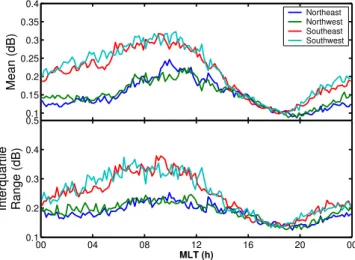
Fig. 5. Top Panel: Daily variation of mean absorption binned by
IMF clock angle quadrants: North-east (blue), north-west (green), south-east (red), south-west (cyan). Bottom Panel: the inter-quartile range of the corresponding distributions.
So far the dependence of energetic particle precipitation (with auroral cosmic noise absorption acting as a proxy) on geomagnetic activity and solar wind speed has been presented. The interplanetary magnetic field also leads to changes in the geomagnetic activity and particle precipita-tion in the ionosphere. The absorpprecipita-tion data for 1995 to 2001 are now sorted by IMF (Bz,By) clock angle quadrant; Fig. 5 (top panel) displays four absorption curves resulting from this binning, with each showing the variation of the mean absorption with magnetic local time. Those curves for north-ward IMF (east is blue and west is green) show very similar variations, with the familiar diurnal variation. For the west-ern values there is a slight increase in the absorption around midnight over the eastern counterpart, leading to an apparent earlier increase in the high morning values. The usual mini-mum is still in the evening sector (≈18:00 to 20:00 MLT).
For the southward-directed IMF; red and cyan indicate eastward and westward directions of theBy component re-spectively. Large rises in absorption levels over the north-ward IMF are evident. Absorption greater than 0.2 dB be-gins around midnight and stretches into the morning sector, increasing to a plateau of ≈0.3 dB at 06:30 MLT.
Follow-ing the usual rapid drop in the afternoon sector, the absorp-tion reaches a minimum of∼0.1 dB in both cases at about
−2 −1.5 −1 −0.5 0 0.5 0
2 4 6 8
00−03 MLT Kp
−2 −1.5 −1 −0.5 0 0.5 0
2 4 6 8
03−06 MLT
−2 −1.5 −1 −0.5 0 0.5 0
2 4 6 8
06−09 MLT Kp
−2 −1.5 −1 −0.5 0 0.5 0
2 4 6 8
09−12 MLT
−2 −1.5 −1 −0.5 0 0.5 0
2 4 6 8
12−15 MLT Kp
−2 −1.5 −1 −0.5 0 0.5 0
2 4 6 8
15−18 MLT
−2 −1.5 −1 −0.5 0 0.5 0
2 4 6 8
18−21 MLT Kp
log
10(Absorption)
−2 −1.5 −1 −0.5 0 0.5 0
2 4 6 8
21−24 MLT
log
10(Absorption)
Fig. 6.Log of the mean (blue crosses) and median (red circles)
val-ues of absorption in eachKpbin plotted against the corresponding
Kp. The two straight lines are linear fits to the data and the dashed
black curves represent the log of±1 standard deviation about the
mean. Kpbins that contain less than 50 data points have been
ex-cluded from contributing to the curve fitting.
4 Discussion
4.1 Diurnal variation
The local time dependence of absorption is a well-known phenomenon (e.g. Hartz et al., 1963). Previous studies found that the strongest absorption occurs in the morning sector extending back towards midnight and slightly beyond. In-vestigations by Driatsky (1966) and Hargreaves and Cow-ley (1967) demonstrated that the absorption close to mid-night showed a peak rather than the smooth decay into the evening sector indicated by other studies. The relative size and appearance of the maxima (pre-noon and pre-midnight) depends on the method by which the statistics are compiled (Hargreaves, 1969). Absorption in the pre-midnight sector is attributed to the precipitation of electrons directly associated with substorm activity (e.g. Ansari, 1964; Ranta et al., 1981), and the precipitation in the morning sector has often been as-sociated with the eastward drift of electrons (Kavanagh et al., 2002 and references therein) following substorm injection. Thus, it is the absorption around midnight that is considered
Table 1.Gradient (S) and intercept (I) values for the fits to Eq. (1)
for both mean and median absorption for data in Fig. 6.
MLT (hours) Mean Median
S I S I
00:00–03:00 0.201 −1.325 0.245 −1.481
03:00–06:00 0.235 −1.358 0.275 −1.505
06:00–09:00 0.240 −1.286 0.277 −1.445
09:00–12:00 0.242 −1.189 0.250 −1.289
12:00–15:00 0.179 −1.106 0.211 −1.286
15:00–18:00 0.067 −1.042 0.098 −1.177
18:00–21:00 0.046 −1.140 0.067 −1.255
21:00–24:00 0.169 −1.289 0.197 −1.428
to be of premier geophysical importance, however, for prac-tical purposes (e.g. HF communication circuits) the morn-ing values are also of interest. Since the current study uses 10-min resolution data to determine the mean values at each magnetic local time, it is less sensitive to the short duration (≈1–5 min) spikes, thus de-emphasizing the midnight peak.
Figure 2 clearly demonstrates the diurnal variation observed in the central beam of IRIS; a strong morning peak following a smooth rise from the pre-midnight sector. Gross features in the distributions should correlate well between individual studies, however, any comparisons between the different sta-tistical studies must take into account the method by which the data were collected.
4.2 Geomagnetic control
Magnetospheric influence on auroral absorption was estab-lished in the early days of riometry (e.g. Parthasarathy and Reid, 1967). Figure 3 shows how with increasing MLT the distribution spreads to higher absorption values at lowerKp until the afternoon when a recovery occurs. A relationship linking geomagnetic activity with absorption for a given lo-cal time and latitude is desirable for prediction purposes. Past authors have attempted to predict auroral radio absorption based upon statistical measurements (e.g. Agy, 1972; Her-man and Vargas-Villa, 1972; Foppiano, 1975; Vondrak et al., 1978 and Foppiano and Bradley, 1984), including terms based upon sunspot number, linking the absorption to the so-lar activity cycle. Hargreaves (1966) determined relation-ships between the absorption and the Kp andAp indices, and later works (Hargreaves et al., 1985, 1987) confirmed this reliance on geomagnetic activity, suggesting that a geo-magnetic term should replace the sunspot dependence in any prediction model.
The investigation by Hargreaves suggested a linear rela-tionship between the log of the median auroral absorption andKpthat was dependent on the time of day:
log10Am=I+S.Kp (1)
geographic), Baie St. Paul (47.37◦,−70.55◦) and Frobisher Bay (63.80◦, −68.70◦) operating at 29.85 MHz. The two lower latitude stations are separated by 38 min of magnetic local time (Baie St. Paul leads Great Whale River), and the data were binned into four ranges of universal time with val-ues of the slope and intercept computed.
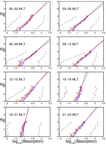
For this study magnetic local time (MLT) bins have been used rather than UT. This makes future comparisons with data from other stations at different locations much simpler, and since absorption is related to substorm activity MLT de-pendence is more likely than UT dede-pendence. As shown in Fig. 3 eight bands of magnetic local time have been chosen to bin the data, corresponding to those intervals over which Kpis calculated. This demonstrated that there is a changing distribution in the absorption at different levels ofKpin each magnetic local time, with the scatter of absorption occupying different ranges. Higher absorption is more likely at some magnetic local times for a givenKp than at other intervals. Figure 6 plots the logarithm of the median and mean absorp-tion values for eachKplevel for each MLT interval. The two colour-coded lines display linear fits to the data for the mean (blue) and median (red) values, and the corresponding coeffi-cients are presented in Table 1. ForKplevels when less than 50 data points occur in each local time bin, the mean and me-dian values are excluded from the fit. On either side of the mean values, the two dashed black lines show the positions of one standard deviation from the mean value; these give an indication of the spread of the data in each of the bins. The differences between the curves in successive time bins sug-gest that the local time dependence is very significant and so using large temporal ranges (e.g. 6 h) is inadvisable. When compared with the results of the investigation by Hargreaves (1966) the gradients of the fit appear reasonable (see Table 2). IRIS is positioned at a latitude between two of the riometers used in the previous study, tending towards the north end of the separation and the gradients (when combined over 6 h) tend towards the northernmost values. Interestingly, the point where the values are markedly different is when the riometers pass through the minimum in the diurnal variation. The ear-lier study used a time bin (18:00–24:00 UT) that spans the rapid decline to, and slow rise from, the minimum (13:00– 19:00 MLT). By weighting the latter half of the time period more than the former, in combining the three-hour bins of the present study, the gradients come into agreement. The dominance of the minimum is unsurprising considering the small effect that geomagnetic activity has on this recurring phenomenon, and it is a clear example of how careful selec-tion of temporal bins is essential to avoid smearing across very different characteristics.
In order to test the accuracy of the fit the empirical equa-tions for the eight time sectors are applied to the Kp data from 1995 to 2001. Correlation coefficients are determined for the observed and estimated absorption for both the mean (r=0.39) and median (r=0.36) cases, and the residuals are
also computed. The means of the residuals are both close to zero, with the median absorption lying closer (−0.002 dB)
than the mean (−0.017 dB). However, the standard
devia-tions of the residuals in both cases demonstrate a wide vari-ability between the observed and calculated CNA (0.238 dB (mean) and 0.263 dB (median)). At times the estimated ab-sorption is>1.7 times the observed value; for an observation of 0.5 dB this produces an error of 0.3 dB at 38.2 MHz. For lower frequencies the error becomes much greater (absorp-tion is approximately inversely propor(absorp-tional to the square of the observing frequency). Restricting the comparison to those data that contribute to determining the empirical equa-tions further tests the correlation. For the range of data rep-resented by the well-defined mean and median values (>50 points in each bin), the correlation is much improved and the spread of the residuals reduces (s.d. ≈0.16 in both cases),
suggesting a better representation. The correlation coeffi-cient is still only 0.53, and more observations during periods of high activity should lead to a better fit of the data; how-ever, it should be considered that the variability of absorption in theKpbins suggests that the statistical mean and median are poor predictors of auroral absorption. The dynamic range of the absorption distribution withKpthat is demonstrated in Fig. 3 has already been mentioned, and this can be seen in the plots of Fig. 6 as well. To address the uncertainty associated with the logarithmic relationship of the absorption, a differ-ent empirical relationship is now suggested; a quadratic is fitted to theKp:
Am=aKp2+bKp+c, (2)
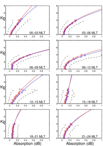
wherea,bandcare constants listed in Table 3 for both the mean and median absorption. Figure 7 displays the local time results of this fit to the data with good results over the range of available data. The black dashed lines are the±1 standard deviation from the mean for eachKp bin. 15:00– 18:00 MLT is at the minimum in the diurnal variation, and the range of absorption values hardly increases as the ac-tivity level rises where the distribution of points suggests a linear fit (e.g.A=bKp+c) that would be more appropriate than the quadratic, and this has been implemented. When a quadratic form is used in this time sector it results in an un-physical variation with rapidly decreasing absorption above Kp=3. Neither the linear nor the squared term dominate to a significant degree in each of the other time ranges, except in the 00:00–03:00 MLT and 12:00–15:00 MLT sectors. At these times it is clear that the relationship is mostly linear with a small nonlinear contribution at highKp. Once again, the fit will be improved when more data at the highest and lowestKpvalues become available.
Testing the relationship in the same manner as for the pre-vious example results in a notably higher correlation between the observed and the calculated data (r=0.51). Also, the
standard deviation of the residuals decreases (s.d.¯0.18 dB). Restricting the comparisons to the data that contribute to the fit leads to a slight improvement (r=0.54, s.d. ≈0.16 dB).
Table 2.Comparing the results of fitting Eq. (1) to the absorption data. The asterisk (*) indicates results from Hargreaves (1966), note that
the two riometers in that study were positioned≈38 min apart in MLT. The values in the two columns under IRIS represent the coefficientS,
from Eq. (1) and Table 1, for the two MLT intervals that best overlap the corresponding periods from the previous study.
Station and Latitude Great Whale river Baie St. Paul IRIS
(aacgm) (67.8◦Mlat)* (60.0◦Mlat)* (65.9◦Mlat)
00:00–06:00 UT 0.113 0.284 0.067 0.197
06:00–12:00 UT 0.216 0.338 0.245 0.275
12:00–18:00 UT 0.284 0.061 0.277 0.250
18:00–24:00 UT 0.080 0.096 0.211 0.098
Table 3. Coefficients for the quadratic fit ofKpto the absorption
values in 8 magnetic local times ranges (from Eq. 2). * indicates where a linear fit has been applied to the data; this is due to the unphysical nature of the quadratic fit in that time sector (see text).
MLT Mean Median
a b c a b c
00:00–03:00 0.005 0.044 0.033 0.002 0.053 0.013
03:00–06:00 0.021 −0.001 0.050 0.017 0.011 0.030
06:00–09:00 0.035 −0.035 0.075 0.032 −0.022 0.047
09:00–12:00 0.040 −0.028 0.086 0.035 −0.026 0.070
12:00–15:00 0.005 0.055 0.064 0.004 0.051 0.037
15:00–18:00 0* 0.002 0.089 0* 0.024 0.061
18:00–21:00 0.004 −0.005 0.080 0.004 −0.004 0.062
21:00–24:00 0.007 0.019 0.049 0.009 0.012 0.037
Figure 3 demonstrated that the absorption has a wide dis-tribution in eachKp bin, but the occurrence is much higher towards the lower end of the absorption scale. This does not exclude high absorption events by any means, but even with high values ofKp there will be many occasions when ab-sorption is low; similar geomagnetic conditions will not nec-essarily return similar absorption levels. When the nature of auroral absorption is considered this becomes less surpris-ing; radio absorption at high latitudes is principally due to the precipitation of energetic particles (electrons of energy >15 keV), and if no such particle population exists on the appropriate magnetic field lines, then no absorption will be observed. Thus, for periods of high geomagnetic activity in close succession the high-energy particle population may be depleted for a time, leading to a significantly reduced absorp-tion level. Alternatively, a lack of absorpabsorp-tion may be a local effect due to an equatorward displacement of the absorption oval as a consequence of an expanded polar cap. In order to make reliable absorption predictions, some term dependent on the recent time history of the magnetic activity must be included in any empirical relationship. This is not included within this paper and instead will be the subject of a future study.
Another important point to note is the variability of ab-sorption on small time scales, especially in the night side
0 0.2 0.4 0.6 0.8 1 0
2 4 6 8
00−03 MLT Kp
0 0.2 0.4 0.6 0.8 1 0
2 4 6 8
03−06 MLT
0 0.2 0.4 0.6 0.8 1 0
2 4 6 8
06−09 MLT Kp
0 0.2 0.4 0.6 0.8 1 0
2 4 6 8
09−12 MLT
0 0.2 0.4 0.6 0.8 1 0
2 4 6 8
12−15 MLT Kp
0 0.2 0.4 0.6 0.8 1 0
2 4 6 8
15−18 MLT
0 0.2 0.4 0.6 0.8 1 0
2 4 6 8
18−21 MLT Kp
Absorption (dB)
0 0.2 0.4 0.6 0.8 1 0
2 4 6 8
21−24 MLT
Absorption (dB)
Fig. 7.Local time plots of the median (red circles) and mean (blue
crosses) absorption against theKp. The curves represent quadratic
fits to the data points and the black dashed lines are±1 standard
deviations about the mean values. Kpbins that contain less than
50 data points have been excluded from contributing to the curve fitting.
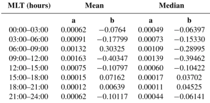
Table 4. Coefficients for the linear fit of the solar wind velocity to absorption values in 8 magnetic local times ranges (from Eq. 3).
MLT (hours) Mean Median
a b a b
00:00–03:00 0.00062 −0.0764 0.00049 −0.06397
03:00–06:00 0.00091 −0.17799 0.00073 −0.15330
06:00–09:00 0.00132 0.30325 0.00109 −0.28995
09:00–12:00 0.00163 −0.40347 0.00139 −0.39462
12:00–15:00 0.00075 −0.10797 0.00060 −0.10422
15:00–18:00 0.00015 0.07162 0.00017 0.03702
18:00–21:00 0.00012 0.00639 0.00011 0.04525
21:00–24:00 0.00062 −0.10117 0.00044 −0.06141
unconfirmed and derived from only 8 of the 12 stations; therefore no fit has been undertaken at this time. Once the data have been confirmed and a longer period is available, AE should prove suitable for attempting a similar process described above forKp.
4.3 Solar wind contributions
Tsurutani et al. (2001) noted that long after the passage of in-terplanetary shocks in two separate events, there was an ap-preciable aurora at dawn, dusk and midnight, recorded by the Ultra Violet Imager carried by the Polar spacecraft. This was attributed to a viscous interaction between the solar wind and the flanks of the magnetosphere, producing either a Kelvin Helmholtz instability (Rostoker et al., 1992) or cross-field diffusion of magnetosheath plasma via ELF/VLF boundary layer wave interactions (Lakhina et al., 2000; Tsurutani and Lakhina, 1997). Either way, small changes in the dynamic pressure, brought about through slight variations in the so-lar wind speed, could result in increased precipitation; this is demonstrated in Fig. 4, where the increased level of solar wind velocity produces large changes in the mean absorp-tion in the morning and midnight sectors, though the major-ity of absorption clusters about 0.1 dB. Once again, there is a strong minimum of the mean CNA in the afternoon/evening sector (15:00–21:00 MLT), and it is unaffected by the in-creasing solar wind velocity. At highVSW the distribution
appears to narrow again, but this is an artfact created by low numbers of data points at the greater speeds. Since the solar wind is credited as being the driving force behind geomag-netic activity, it seems reasonable to link the absorption to the energy input from the solar wind. The study by Harg-reaves (1966) attempted to estimate the total energy of pre-cipitated particles. This relied on the empirical relationship derived by Hargreaves and Sharp (1965), linking the absorp-tion to the square root of the total energy of the precipitated electrons, combined with an expression for the solar wind velocity based onKp andAp. Measurements of the solar wind were made by the Mariner 2 space probe to derive this relationship (Snyder et al., 1963). With the data available
from the ACE and WIND spacecraft it is possible to attempt to link auroral absorption directly with the solar wind veloc-ity. By compiling mean and median absorption values from 50 km/s wide bins, a similar method to the previously imple-mented procedure can be applied to the data. Figure 8 shows the results of the binning with a linear fit to the data of the form:
Am=aVSW+b (3)
Values for the coefficientsaandbare presented in Table 4. The data distribution in the pre-noon sector shows some non-linearity, but this is not repeated to any notable effect in the other local time bins and does not compare with that recorded for theKpbins. The correlation coefficients (r=0.48)
sug-gest a better result than for the originalKpfit, and the stan-dard deviation of the residuals (0.19 dB) is comparable with those of the quadratic relationship inKp. When the relation-ship is computed for only those velocities where more than 50 data points are used to calculate mean and median val-ues, there is no discernable difference in the correlation. The current Eq. (3) will produce unrealistic values for low solar wind velocities (<200 km/s) in most cases; however, in the previous half solar cycle there have been no occurrences of the solar wind dropping below≈250 km/s. Values of
absorp-tion calculated for a solar wind velocity less than 250 km/s should be discounted as extremely unreliable as should val-ues in excess of 800 km/s. It is highly likely that at large velocity, other mechanisms of absorption, such as the sud-den commencement absorption (SCA) and sudsud-den impulse absorption (SIA) (Brown et al., 1961; Brown and Driatsky, 1973), will dominate.
By fitting a quadratic equation as with theKpthe correla-tion changes by only a small amount, and similar results are obtained from comparing the logarithm of the speed and the absorption (e.g.r=0.49). Thus, the simple linear fit to the
solar wind data seems to be the best that can be achieved but results in a relatively weak correlation. It is believed that the important factor that is necessary to improve upon these re-sults is to combine the effects of the IMF (discussed below) with that of the solar wind and to include some term that takes account the recent time history of the solar wind/IMF. This “priming” factor would be related to the storing of en-ergy in the magnetotail prior to release during substorm on-set. Much further work is needed before a reliable prediction model for auroral absorption can be created based on a so-lar wind parameter, though existing absorption models (e.g. Foppiano and Bradley, 1983; Greenberg and La Belle, 2002) have changed from using a solar cycle related term (usually sunspot number) to a geomagnetic dependent value.
4.4 IMF contributions
0 0.2 0.4 0.6 0.8 1 200
400 600 800
00−03 MLT V SW
(km/s)
0 0.2 0.4 0.6 0.8 1 200
400 600 800
03−06 MLT
0 0.2 0.4 0.6 0.8 1 200
400 600 800
06−09 MLT V SW
(km/s)
0 0.2 0.4 0.6 0.8 1 200
400 600 800
09−12 MLT
0 0.2 0.4 0.6 0.8 1 200
400 600 800
12−15 MLT V SW
(km/s)
0 0.2 0.4 0.6 0.8 1 200
400 600 800
15−18 MLT
0 0.2 0.4 0.6 0.8 1 200
400 600 800
18−21 MLT V SW
(km/s)
Absorption (dB)
0 0.2 0.4 0.6 0.8 1 200
400 600 800
21−24 MLT
Absorption (dB)
Fig. 8. Absorption versus solar wind velocity for 8 magnetic
lo-cal time ranges. Mean and median values are lo-calculated for each 50 km/s bin and straight line fits derived. The black dashed lines
represent±1 standard deviation about the mean values. Solar wind
bins that contain less than 50 data points have been excluded from contributing to the curve fitting.
remains very low in the evening sector. A westward IMF ap-pears to favour an increase in absorption over midnight and into the morning sector, perhaps due to the skewing of the field lines (Cowley et al., 1991), leading particles to precip-itate at an earlier local time. To determine whether this is significant on a statistical level the data are subjected to the Kolmogorov-Smirnov significance test (Von Mises, 1964), which tests the hypothesis that two samples are drawn from the same distribution. A significance probability, SP,<0.01 suggests that the samples come from significantly different distributions. For positiveBy, north and southward IMF have been compared. The results show a SP<0.01 from 20:00 to 12:00 MLT, suggesting that the data in this band are from very different distributions. Midnight and morning absorp-tion is highly dependent on the IMF, and the low absorpabsorp-tion values in the afternoon/evening are not; this reinforces the observations that the minimum does not change with either Kp or VSW. Comparing east and west IMF (for southward
Bz) we find SP>0.01 for virtually all of the day, such that no significant conclusion can be drawn about the
possibil-00 04 08 12 16 20 00
0.05 0.1 0.15 0.2 0.25 0.3 0.35 0.4 0.45 0.5
Absorption (db)
MLT (h)
BZ > 4
4 ≥ B
Z > 2
2 ≥ B
Z > 0
0 ≥ B
Z > −2
−2 ≥ B
Z > −4
B
Z≤ −4
Fig. 9. Ten-min averaged absorption binned by IMFBz. A
north-ward IMF does not affect the absorption, whereas increasingly
neg-ativeBzincreases the level of absorption during the night and
morn-ing sectors.
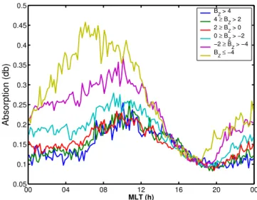
ity ofByhaving an effect on the absorption. Discarding the Byparameter as insignificant for these purposes, the zenithal absorption can be binned byBz, in order to further investi-gate the dependence. Figure 9 shows that when the mean absorption is binned byBzthere is a definite effect for nega-tive values, both around midnight and in the morning sector. Once again the field strength does not affect the level of the minimum. In addition a northward IMF does not seem to radically affect the absorption as southward does; the curves for positiveBz cluster below a 0.25 dB maximum, with lit-tle difference between each range. Those curves forBz<0 display a definite trend with increasingly higher values of ab-sorption for successively negative values ofBz. Thus, the ab-sorption distribution is obviously dependent on theZ compo-nent of the IMF, just as should be expected, since absorption is substorm dependant. This approach does not account for transient effects in the absorption, such as those reported by Nishino et al. (1999) for a rectified response to north/south turnings in the IMF. That example was related to increases in field-aligned currents close to the open/closed field line boundary, whereas the general increase here is likely related to the occurrence of substorm activity for negative IMF.
An inspection of the IMFBzversus the solar wind speed (data not shown) shows no bias in the data, so high velocities occur for both positive and negativeBz. It should be possible to develop a relationship for the dependence of absorption on the IMF that could further be improved by separating the effects of the solar wind speed. This would go a long way to establishing a more accurate model for predicting auroral absorption and will be the subject of a future study.
4.5 The diurnal minimum
Figure 2 demonstrated the large decrease in absorption at around 18:00 MLT. Similarly, when the data are binned by Kp the minimum is recurring, always reaching down to
∼0.15 dB. In fact, this occurs for every level of solar wind
speed (e.g. Fig. 4) and also the for IMF (Fig. 5). There is no significant difference between the distributions at the mini-mum when comparing north and south-directed IMF; quite obviously, the minimum is unaffected by geomagnetic, solar wind or IMF activity. The exact mechanics behind the diur-nal minimum are beyond the scope of this study; suffice to say that the minimum is a recurring statistical phenomenon that is likely related to a combination of the loss of drift-ing electrons (through earlier precipitation and radial diffu-sion) and the remaining population becoming stably trapped in the magnetosphere. For this study it is only necessary to acknowledge the existence of the minimum as a limiting case on the local time dependence of the relationship between ab-sorption andKpand the solar wind velocity.
5 Conclusions
Data have been combined from 7 years of continuous ob-servations of the auroral absorption from a single imaging riometer (IRIS) using the narrow zenithal beam to investi-gate the dependence of absorption on geomagnetic and solar wind parameters. 1995 to 2001 covers the ascending phase of solar cycle 23. The narrow beam offers a better estimate of the height-integrated absorption over broad beam riome-ter observations, since it integrates over a smaller portion of the sky. Through the sorting of absorption into bins of corre-spondingKp a quadratic empirical relationship between the two parameters is derived and provides a better correlation of calculated and observed absorption than the linear fit based on the logarithm of the absorption. The local time depen-dence of absorption is so clear that the possibility that differ-ent types of fits to the data in each MLT bracket should not be discounted. Any future investigation of this nature should take this into account.
For the first time a linear relationship between the solar wind velocity and the auroral absorption has been derived. This is based upon direct solar wind observations rather than estimates based on theKp index. Combining the observa-tions results in a reasonable correlation; however, it is clear that some other factor must play a role in the relationship. It appears that a southward-orientated IMF plays a signifi-cant role in precipitation in the auroral zone, but the eastward component does not have a statistical effect on the mean ab-sorption. Deriving a relationship betweenBzand absorption after the effects of the solar wind speed have been removed will be the focus of a future study.
The afternoon/evening minimum in the diurnal vari-ation of absorption appears to be a strongly consis-tent phenomenon. Absorption virtually disappears around 18:00 MLT regardless of the geomagnetic, solar wind or IMF activity. This is likely related to the loss of the bulk of drifting particles. The remaining flux of electrons is probably lower
than the critical flux necessary for whistler-mode instability that drives enhanced precipitation in the dayside magneto-sphere (Kennel and Petschek, 1966; Coroniti and Kennel, 1970). The mechanisms of this effect are beyond the scope of the current study, and for the purposes of prediction it is only necessary to acknowledge the fact that the minimum occurs. Although apparently reasonable fits to the mean and me-dian absorption can be found for bothKpand the solar wind speed, the variability of the absorption still leads to prob-lems. Low absorption is still likely even when geophysical activity is high, since absorption is highly dependent on the population of energetic particles in the magnetosphere; with-out fluxes of electrons (energies >15 keV) no appreciable absorption is possible. Thus current, global models of ab-sorption based on onlyKp values are somewhat unreliable. Methods to improve such a model must take into account past levels of geomagnetic activity, absorption and some other measure of the energy stored in the magnetotail (e.g.Bz). A detailed study of how absorption responds during geomag-netic storms would be especially useful, linking the observa-tions to past levels of activity, as indicated not only byKp andDst but also by the IMF and solar wind speed. If this is done then with the large array of riometers available in both hemispheres and the catalogue of data, a suitable global em-pirical prediction model could be defined.
Acknowledgements. The Imaging Riometer for Ionospheric Studies
(IRIS) is operated by the Department of Communications Systems at Lancaster University (UK), funded as a UK National Facility by the Particle Physics and Astronomy Research Council (PPARC) in collaboration with the Sodankyl¨a Geophysical Observatory. R. Lep-ping and K. Ogilivie at NASA/GSFC provided wind data through CDAWeb. We thank the ACE SWEPAM and MAG instrument teams and the ACE Science Center for providing the ACE Level 2 data. AJK is indebted to both PPARC and the Rutherford Ap-pleton Laboratories for a CASE research studentship during which the bulk of this work was completed at Lancaster University. AS is supported on a PPARC research studentship at Lancaster University and EEW was funded by a PPARC research studentship at the Uni-versity of Leicester. We gratefully acknowledge Dr. Gang Lu for reviewing this manuscript at HAO before submission and for her subsequent comments.
The Editor in Chief thanks T. Yeoman for his help in evaluation this paper.
References
Agy, V.: A model for the study and prediction of auroral effects on HF radar, Proc. AGARD conference “Radar propagation in the Arctic, AGARD-CP-97, 32-1, 1972.
Ansari, Z. A.: The aurorally associated absorption of cosmic noise at College Alaska, J. Geophys. Res., 69, 4493–4513, 1964. Baker, K. B. and Wing, S.: A new magnetic coordinate system for
conjugate studies at high latitudes, J. Geophys. Res., 94, 9139-9143, 1989.
Brown, R. R., Hartz, T. R., Landmark, B., Leinbach, H., and Ortner, J.: Large-Scale Electron Bombardment of the Atmosphere at the Sudden Commencement of a Geomagnetic Storm, J. Geophys. Res., 66, 1035-1041, 1961.
Browne, S., Hargreaves, J. K., and Honary, B.: An Imaging Riome-ter for Ionospheric Studies, Elect. Comm. Eng. J., 7, 209-217, 1995.
Coroniti, F. V. and Kennel, C. F.: Electron Precipitation Pulsations, J. Geophys. Res. 75, 1279–1289,1970.
Cowley, S. W. H., Morelli, J. P., and Lockwood, M.: Dependence of convective flows and particle precipitation in the high latitude
ionosphere on the X and Z-components of the interplanetary
magnetic field, J. Geophys. Res., 96, 5557-5564, 1991.
Detrick, D. L. and Rosenberg, T. J.: A Phased-Array Radiowave Imager for Studies of Cosmic Noise Absorption, Radio Science, 25, 325-338, 1990.
Driatsky, V. M.: Study of the space and time distribution of auroral absorption according to observations of the riometer network in the arctic, Geomagnetism and Aeronomy, 6, 828–834, 1966. Foppiano, A. J.: A new method for predicting the auroral absorption
of HF sky waves, CCIR Interim Working Party 6/1. Docs. 3 and 10, International Telecommunication Union, 1975.
Foppiano, A. J. and Bradley, P. A.: Prediction of auroral absorption of high-frequency waves at oblique incidence, Telecommun. J., 50, 547–560, 1983.
Foppiano, A. J. and Bradley, P. A.: Day to day variability of riome-ter absorption, J. Atmos. Terr. Phys., 46, 689–696, 1984. Foppiano, A. J. and Bradley P. A.: Morphology of background
au-roral absorption, J. Atmos. Terr. Phys. 47, 663–674, 1985. Greenberg, E. M. and LaBelle, J.: Measurement and modeling of
auroral absorption of HF radio waves using a single receiver, Ra-dio Sci., 37, 6, 1–12, 2002.
Hargreaves, J. K.: On the variation of auroral radio absorption with geomagnetic activity, Planet. Space. Sci. 14, 991–1006, 1966. Hargreaves, J. K.: Auroral Absorption of HF Radio Waves in the
Ionosphere: A Review of Results from the First Decade of Ri-ometry, Proceedings of the IEEE, 57, 1348-1373, 1969. Hargreaves, J. K. and Cowley, F. C.: Studies of Auroral
Absorp-tion Events at Three Magnetic Latitudes – I. Occurrence and Sta-tistical Properties of the Events, Planet. Space Sci., 1571–1583, 1967.
Hargreaves, J. K. and Sharp, R. D.: Electron Precipitation and Iono-spheric Radio Absorption in the Auroral zones, Planet. Space. Sci., 13, 1171–1183, 1965.
Hargreaves, J. K., Feeney, M. T. and Burns, C. J.: Statistics of auroral radio absorption in relation to prediction models, Proc. 36th symposium of the electromagnetic wave propagation panel, AGARDS-CP-382, 1–10, 1985.
Hargreaves, J. K., Feeney, M. T., Ranta, H., and Ranta, A.: On the prediction of auroral radio absorption on the equatorial side of the absorption zone, J. Atmos. Terr. Phys., 49, 259–272, 1987. Hartz, T. R., Montbriand, L. E., and Vogan, E. L.: A study of auroral
absorption at 30 Mc/s, Can. J. Phys., 41, 581–595, 1963. Herman, J. R. and Vargas-Villa, R.: Investigation of auroral
iono-spheric and propagation phenomena related to the Polar Fox II experiment, Analytical Systems Corporation, Report ASCR-72-62, 1972.
Holt, O., Landmark, B., and Lied, F.: Analysis of riometer observa-tions obtained during polar radio blackouts, J. Atmos. Terr. Phys., 23, 229–248, 1961.
Kavanagh, A. J., Honary, F., McCrea, I. W., Donovan, E., Wood-field, E. E., Manninen, J., and Anderson, P. C.: Substorm related changes in precipitation in the dayside auroral zone - a multi in-strument case study, Ann. Geophys., 20, 1321–1334, 2002. Kennel, C. F. and Petschek, H. E.: Limit on stably trapped particle
fluxes, J. Geophys. Res., 71, 1–28, 1966.
Lakhina, G. S., Tsurutani, B. T., Kojima, H., and Matsumoto, H.: “Broadband” plasma waves in the boundary layers, J. Geophys. Res., 105, 27 791–27 831, 2000.
Lepping, R. P., Acuna, A. H., Burlaga, L. F., Farrell, W. M., Slavin, J. A., Schatter, K. H., Mariani, F., Ness, N. F., Neubauer, F. M., Whang, Y. C., Byrnes, J. B., Kennon, R. S., Panetta, P. V., Scheifele, J. and Worler, E. M.: The WIND magnetic field inves-tigation, Space Sci. Rev., 71, 207–229, 1995.
McComas, D. J., Bame, S. J., Barker, P., Feldman, W. C., Phillips, J. L., Riley, P., and Griffee, J. W.: Solar Wind Electron Proton Alpha Monitor (SWEPAM) for the Advanced Composition Ex-plorer, Space Sci. Rev., 86, 563–612, 1998.
Nishino, M., Nishitani, N., Sato, N., Yamagishi, H., Lester, M., and Holtet, J. A.: A rectified response of daytime radio wave absorp-tion to southward and northward excursions during northward interplanetary magnetic field: A case study, Adv. Polar Upper Atmos. Res., 13, 139–153, 1999.
Ogilivie, K. W., Chornay, D. J., Fritzenreiter, R. J., Hunsaker, F., Keller, J., Lobell, J., Miller, G., Scudder, J. D., Sittler, Jr., E. C., Torbert, R. B., Bodet, D., Needell, G., Lazarus, A. J., Steinberg, J. T., Tappan, J. H., Mavretic, A., and Gergin, E.: SWE, A com-prehensive plasma instrument for the WIND spacecraft, Space Sci. Rev. 71, 55–77,1995.
Parthasarathy, R. and Reid, G. C.: Magnetospheric Activity and its consequences in the auroral zone, Planet. Space Sci., 15, 917– 929, 1967.
Ranta, H., Ranta, A., Collis, P. N., and Hargreaves, J. K.: Develop-ment of the Auroral Absorption Substorm: Studies of Pre-onset Phase and Sharp Onset Using an Extensive Riometer Network, Planet. Space Sci., 1287–1313, 1981.
Rostocker, G., Jackel, B., and Arnoldy, R. L.: The relationship of periodic structure in auroral luminosity in the afternoon sector of ULF pulsations, Geophys. Res. Lett., 19, 613–616, 1992. Smith, C. W., L’Hereux, J., Ness, N. F., Acuna, M. H., Burlaga, L.
F., and Schiefle, J.: The ACE Magnetic Fields Experiment, Space Sci. Rev., 86, 613–632, 1998.
Snyder, C. W., Neugebauer, M., and Rae, U. R.: The Solar Wind Velocity and Its Correlation with Cosmic ray Variations and with Solar and geomagnetic activity, J. Geophys. Res., 68, 6361– 6370, 1963.
Tsurutani, B. T. and Lakhina, G. S.: Some basic concepts of wave-particle interactions in collisionless plasmas, Rev. Geophys., 35, 491–501, 1997.
Tsurutani, B. T., Zhou, X. Y., Arballo, J. K., Gonzalez, W. D., Lakhina., G. S., Vasyliunas, V., Pickett, J. S., Araki, T., Yang, H., Rostocker, G., Hughes, T. J., Lepping, R. P., and Berdichevsky, D.: Auroral zone dayside precipitation during magnetic storm initial phases, J. Atmos. Sol. Terr. Phys., 63, 513–522, 2001. Vondrak, R. R., Smith, G., Hatfield, V. E., Tsunoda, R. T., Frank,
V. R., and Perreault, P. D.: Chantika model of the high-latitude ionosphere for application to HF propagation prediction. Rome Air Development Center Technical Report, RADC-TR-78-7, 1978.