Review and classification of indicators of green water availability and scarcity

(1)

www.hydrol-earth-syst-sci.net/19/4581/2015/ doi:10.5194/hess-19-4581-2015

Review and classification of indicators of green water

availability and scarcity

J. F. Schyns, A. Y. Hoekstra, and M. J. Booij

Twente Water Centre, University of Twente, Enschede, the Netherlands Correspondence to:J. F. Schyns ([email protected])

Received: 20 May 2015 – Published in Hydrol. Earth Syst. Sci. Discuss.: 11 June 2015 Revised: 4 November 2015 – Accepted: 5 November 2015 – Published: 18 November 2015

Abstract.Research on water scarcity has mainly focussed on blue water (ground- and surface water), but green water (soil moisture returning to the atmosphere through evaporation) is also scarce, because its availability is limited and there are competing demands for green water. Crop production, graz-ing lands, forestry and terrestrial ecosystems are all sustained by green water. The implicit distribution or explicit allocation of limited green water resources over competitive demands determines which economic and environmental goods and services will be produced and may affect food security and nature conservation. We need to better understand green wa-ter scarcity to be able to measure, model, predict and handle it. This paper reviews and classifies around 80 indicators of green water availability and scarcity, and discusses the way forward to develop operational green water scarcity indica-tors that can broaden the scope of water scarcity assessments.

1 Introduction

Freshwater is a renewable resource that is naturally replen-ished over time when moving through the hydrological cycle (Oki and Kanae, 2006; Hoekstra, 2013). Precipitation forms the input of freshwater on land. Subsequently, it takes the blue or the green pathway back to the ocean and atmosphere before eventually returning as precipitation again (Falken-mark, 2003; Falkenmark and Rockström, 2006, 2010). The water that runs off to the ocean via rivers and groundwater is called the blue water flow. The green water flow is formed by the water that is temporarily stored in the soil and on top of vegetation and returns to the atmosphere as evaporation in-stead of running off (Hoekstra et al., 2011). As suggested by Savenije (2004), in this paper we use the term evaporation

(instead of the often used term evapotranspiration) to refer to the vapour flux from land to atmosphere, which includes soil evaporation, evaporation of intercepted water, transpira-tion and in some cases (e.g. rice or swamp vegetatranspira-tion) open-water evaporation. About three-fifth of the precipitation over land takes the green path and two-fifth the blue path (Oki and Kanae, 2006).

Both blue and green water flows are made productive for human purposes. Blue water is used for industrial and do-mestic purposes and irrigation in agriculture. Green water sustains crop production, grazing lands, forestry and terres-trial ecosystems (Rockström, 1999; Rockström et al., 1999; Savenije, 2000; Gerten et al., 2005). These systems pro-vide food, fibres, biofuels, timber and livestock products and other ecosystem services humans benefit from (Millennium Ecosystem Assessment, 2005; Gordon et al., 2010).

Although freshwater is renewable, this does not mean that its availability is unlimited. In fact, freshwater is also a fi-nite resource (Hoekstra, 2013). Over a certain period, there falls a certain amount of precipitation. This limits both blue and green water availability in time. Human society cannot appropriate more water than is available. The finiteness of freshwater, in combination with the various competing de-mands for water, makes water a scarce resource.

(2)

en-ergy production from biomass create additional pressure on water and land (Hejazi et al., 2014). Additionally, a changing climate with increased variability and more extremes (IPCC, 2013) amplifies water scarcity (WWAP, 2014).

Given that green and blue water resources are limited and there are competing demands for both, green water as well as blue water are scarce. Therefore, it is surprising that re-search and debate on water scarcity have been, and still are, mainly focussed on blue water (Vörösmarty et al., 2000, 2010; Rijsberman, 2006; Wada et al., 2011; Hoekstra et al., 2012; WWAP, 2014, 2015). Although the importance of green water has increasingly gained acceptance since Falken-mark (1995) drew attention to it in the mid-1990s (Savenije, 2000; Rockström, 2001; Rijsberman, 2006; Liu et al., 2009; Hanasaki et al., 2010; Hoekstra and Mekonnen, 2012), the notion of green water scarcity is addressed in the literature to a limited extent (Falkenmark et al., 2007; Falkenmark, 2013a, b). While the need to incorporate green water in wa-ter scarcity indicators and assessments has already been ex-pressed since the beginning of this millennium (Savenije, 2000; Rockström, 2001; Rijsberman, 2006; Falkenmark and Rockström, 2006), only a few attempts have been made so far in the form of combined green–blue water scarcity assess-ments (Rockström et al., 2009; Gerten et al., 2011; Kummu et al., 2014) (discussed in detail in Sect. 3.2).

Green water scarcity refers to the competition over lim-ited green water resources and allocation over competing demands. This allocation occurs mostly implicitly and indi-rectly, since generally it is land that is been allocated to a certain use. This indirectness of allocation, together with the absence of a price, makes green water scarcity invisible in our economy. This does not mean, though, that green water resources are not scarce, since using green water for one pur-pose makes it unavailable for another purpur-pose. We need to measure how scarce green water is in order to answer ques-tions like following: Can we produce enough food, feed, fi-bres, bioenergy and forestry products with limited availabil-ity of water resources and suitable land? How can we do so without compromising natural ecosystems and other sectors that put a claim on water and land resources? For study-ing these crucial questions, a sole assessment of blue water scarcity is insufficient.

Therefore, it is due time that more attention is given to green water scarcity and how we can measure it. In this re-view, we make an inventory of existing indicators of green water availability and scarcity, and classify them based on their scope and purpose of measurement. The classification allows us to discuss similarities and differences between in-dicators and give advice on how the various indicator classes could be used to measure different kinds of green water avail-ability or scarcity. This is useful in order to properly include limitations in green water availability in water scarcity as-sessments.

A review of green water scarcity indicators is new in its kind. Past reviews of water scarcity indicators (Savenije,

2000; Rijsberman, 2006) date back a while and hence do not include recent developments in the field, especially those related to the inclusion of green water. There exist multi-ple reviews of indicators of aridity (Wallén, 1967; Walton, 1969; Stadler, 2005) and drought (World Meteorological Or-ganization, 1975; Wilhite and Glantz, 1985; Maracchi, 2000; Tate and Gustard, 2000; Keyantash and Dracup, 2002; Heim, 2002; Hayes, 2007; Kallis, 2008; Mishra and Singh, 2010; Sivakumar et al., 2011). We classify and discuss these indi-cators in an overarching way. First, we discuss the multiple dimensions of water availability and scarcity, and sharpen the scope of this review (Sect. 2). Next, we classify and review green water availability and scarcity indicators (Sect. 3). Fi-nally, we draw conclusions and discuss future research direc-tions (Sect. 4).

2 Multiple aspects of water availability and scarcity The concepts of water availability and scarcity are examined in Sect. 2.1 to 2.4. We will reflect on these concepts in broad terms, not yet focussing on green water. In Sect. 2.5, we de-tail the scope of the indicators discussed in this paper. 2.1 Water availability and scarcity

A straightforward definition of water scarcity is “an excess of water demand over available supply” (FAO, 2012). Various other definitions of water scarcity exist that aim to be more inclusive.

“An imbalance between supply and demand of freshwa-ter in a specified domain (country, region, catchment, river basin, etc.) as a result of a high rate of demand com-pared with available supply, under prevailing institutional ar-rangements (including price) and infrastructural conditions.” (FAO, 2015)

“When an individual does not have access to safe and af-fordable water to satisfy her or his needs for drinking, wash-ing or their livelihoods we call that person water insecure. When a large number of people in an area are water insecure for a significant period of time, then we can call that area water scarce.” (Rijsberman, 2006)

Considering these definitions, we can conclude that wa-ter scarcity is not something that is experienced by a sin-gle person at a particular moment (day or week). Rather, it is experienced by a larger community within a certain geo-graphic area (e.g. catchment or country) and relates to larger timescales (months or years).

(3)

Until now we have spoken about physical water scarcity, referring to the situation where there is insufficient water to meet human demand. If human, institutional and finan-cial capital limit access to water, the term economic wa-ter scarcity applies (Seckler et al., 1999; Molden, 2007). In a broader sense, Ohlsson (2000) defines social resource scarcity as the situation in which social resources required to successfully adapt to physical water scarcity fall short. 2.2 Relative and absolute water scarcity

According to economic theory, water is a scarce good be-cause it carries opportunity costs, which are the benefits fore-gone from possible alternative uses of the water (FAO, 2004). This is a form of “relative scarcity” based on the assumption of substitutability of goods (Baumgärtner et al., 2006). Water can be scarce in the relative sense also in water-abundant ar-eas, because allocating water to purpose A implies it cannot be allocated to purpose B. In other words, water for purpose A is scarce in relation to water for other purposes. In com-mon language we are inclined to say that sometimes water is scarce and at other times it is not. In economic sense, water is always scarce; the degree of water scarcity can vary though, and it can even be zero if alternative uses and thus competi-tion is absent.

We speak of “absolute scarcity” when according to Baumgärtner et al. (2006) “scarcity concerns a non-substitutable means for satisfaction of an elementary need and cannot be levied by additional production”. This means that in an area with a limited amount of water resources (that cannot be increased), at a certain level of consumption, water for elementary purposes (e.g. drinking and food production) will no longer be substitutable with water used for less es-sential purposes. In this case, there is absolute scarcity of wa-ter. Whether water is scarce in the absolute or relative sense thus depends on the degree of water scarcity: relative water scarcity turns into absolute scarcity when the boundaries of water exploitation are approached.

2.3 Blue and green water

Freshwater essentially stems from precipitation, which parti-tions into green and blue water (Falkenmark and Rockström, 2006, 2010). As discussed in the introduction of this paper, water availability and scarcity can pertain to both blue or green water resources, separately or in combination (Falken-mark, 2013a).

In contrast to the clear definition of blue water, various definitions of green water exist, defining it as an inflow (pre-cipitation), a stock (rainwater in the soil) or an outflow (evap-oration of rainwater). Often, the term green water is used to refer to “rainwater stored in the soil” or more specifically plant-available soil moisture in the unsaturated zone (Falken-mark et al., 2007; Falken(Falken-mark, 2013a); in this context the term green water is interpreted as a stock. Commonly, the

distinction is made between green water stock and green wa-ter flow (Falkenmark and Rockström, 2006, 2010). The lat-ter is an outflow, usually defined as actual evaporation over land (referring to the entire land–atmosphere vapour flux; see comment in the introduction), but it has also been defined as transpiration only (Savenije, 2000). Furthermore, some au-thors include precipitation (i.e. an inflow) in the definition of green water (Weiskel et al., 2014). The latter is in contrast with the definition of Falkenmark and Rockström (2006) (ad-hered to in this paper) that precipitation is the undifferenti-ated freshwater resource. Scholars who have tried to quantify green water availability in water scarcity assessments defined it as the actual evaporation flux over land to the atmosphere (Rockström et al., 2009; Gerten et al., 2011; Kummu et al., 2014) (Sect. 3).

While not always made explicit in definitions, an accu-rate description of the green water storage and flow excludes the part of the storage and vapour flow that originates from blue water resources, which have been redirected to the soil moisture stock by means of irrigation, capillary rise or natu-ral flooding (Hoekstra et al., 2011). In such cases, the green and blue contributions to the soil moisture can be tracked with a model-based water balance approach (see Chukalla et al., 2015).

2.4 Water quantity and quality

Water scarcity is not only a function of the quantity of the water resource in relation to the demand, but also the qual-ity of the resource in relation to the required qualqual-ity for its end purpose (Pereira et al., 2002). If there is sufficient water available for a certain purpose, but it is polluted to such an extent that it is not usable for that purpose, then water can be considered scarce as long as the means are not available for cleaning the water to a desirable level. Pollution of water resources can thus aggravate water scarcity (FAO, 2012).

Water quality in the case of green water differs from that of blue water. The quality of green water depends on soil prop-erties such as nutrient availability, nutrient retention capac-ity and the presence of salts and toxic substances. However, close ties with blue water quality do exist. For example, blue water used for irrigation can increase soil salinity when the water is brackish or saline and it can also flush out excess nutrients and other substances.

2.5 Scope of the review and classification

(4)

in-dicators focussing on blue water that are outside the scope of this paper are the following:

– Hydrological drought: concerns the effects of dry pe-riods on surface and subsurface flows and stocks and is therefore related to blue water. Examples of associ-ated indicators are surface water supply index (Shafer and Dezman, 1982), Palmer Hydrological Drought In-dex (Karl, 1986) and several indicators reviewed by Smakhtin (2001).

– Blue water scarcity: measures demand for blue water re-sources versus blue water availability and is thus purely related to blue water. Examples of associated indica-tors are the water crowding indicator (Falkenmark et al., 1989), the withdrawal-to-discharge ratio (Vörösmarty et al., 2000), water poverty index (Sullivan et al., 2003), water stress indicator (Smakhtin et al., 2004), water stress index (Pfister et al., 2009), dynamic water stress index (Wada et al., 2011) and blue water scarcity (Hoek-stra et al., 2012). Note that some of these indicators also incorporate more than only physical elements of water scarcity (e.g. water poverty index).

The concepts related to broader forms of water scarcity than physical water scarcity that are outside the scope of this paper are the following:

– Socio-economic drought: concerns imbalances in sup-ply and demand of economic goods due to the physi-cal characteristics of drought (Wilhite and Glantz, 1985; American Meteorological Society, 2013) with effects on the economy and society. The American Meteorologi-cal Society (2013) mentions the following effects: loss of income from lower crop yields, reduced spending in rural communities, health issues and mass migration. – Social resource scarcity: see Sect. 2.1.

Furthermore, the review and classification in this paper ex-cludes indicators that measure drought by combining mul-tiple drought indicators (classified individually) and some-times other information such as land use maps. Examples of such indicators are the US Drought Monitor (Svoboda et al., 2002) and the Vegetation Drought Response Index (Brown et al., 2008).

3 Green water availability and scarcity indicators We have identified around 80 indicators of green water avail-ability and scarcity, which we classify into the following cat-egories:

1. Green water availability indicators show whether green water availability is low or high and are insensitive to actual water demand. In other words, when the water

demand increases, indicator values will not reflect this. Within this category we distinguishabsoluteand rela-tivegreen water availability indicators:

(a) Absolute green water availability indicators mea-sure actual conditions of green water availability (in an absolute sense).

(b) Relative green water availability indicators measure actual conditions of green water availability com-pared to conditions that are perceived as normal, which is often defined as the climate-average or me-dian value of the variable of interest.

Note that this distinction between absolute and relative in-dicators is unrelated to and different from the concepts of relative and absolute scarcity earlier discussed in Sect. 2.2.

1. Green water scarcity indicators incorporate elements of both water availability and demand and therefore re-spond – in contrast to green water availability indicators – to changes in water demand as well. We distinguish three different options to measure green water scarcity conceptually (explanation in Sect. 3.2):

(a) green water crowding;

(b) green water requirements for self-sufficiency versus green water availability;

(c) actual green water consumption versus green water availability.

The usage of terms like water availability and water demand can be confusing because in different contexts they have dif-ferent meanings. The term green water availability is basi-cally used in two different ways. When we speak of green water availability indicators (Sect. 3.1), we refer to indicators that measure the availability of green water in one way or an-other, without considering availability in relation to an actual demand for green water. This is in contrast with green water scarcity indicators that always compare demand to availabil-ity. In the case of green water scarcity indicators, the term green water availability specifically refers to the part of the green water flow available for biomass production for human purposes (Sect. 3.2). Also the term demand occurs in two dif-ferent contexts. When we speak of demand in the context of green water scarcity, we refer to the demand for green water, associated with the production of biomass for human pur-poses. In the discussion of agricultural drought indicators in Sect. 3.1, the term crop moisture/evaporation/water demand is used to refer to the water needs of the crop for non-water limited growth.

(5)

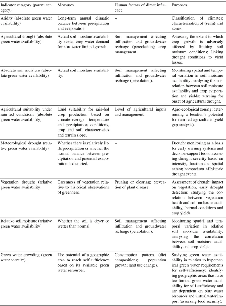
Table 1.Overview of indicator categories.

Indicator category (parent cat-egory)

Measures Human factors of direct

influ-ence

Purposes

Aridity (absolute green water availability)

Long-term annual climatic

balance between precipitation and evaporation.

– Classification of climates;

characterization of (semi)-arid zones.

Agricultural drought (absolute green water availability)

Actual soil moisture availabil-ity versus crop water demand for non-water limited growth.

Soil management affecting

infiltration and groundwater recharge (percolation); crop management.

Assessing the extent to which

crop growth is adversely

affected by limiting soil

moisture conditions; linking drought conditions to yield losses.

Absolute soil moisture (abso-lute green water availability)

Actual soil moisture availabil-ity.

infiltration and groundwater recharge (percolation).

Monitoring spatial and tempo-ral variation in soil moisture availability; analysing the cor-relation between soil moisture availability and crop evapora-tion and yields; warning for onset of agricultural drought.

Agricultural suitability under rain-fed conditions (absolute green water availability)

Land suitability for rain-fed

crop production based on

climate-average temperature

and precipitation conditions, crop and soil characteristics and terrain slope.

Level of agricultural inputs and management.

Agro-ecological zoning; deter-mining a location’s potential for rain-fed agriculture (yield gap analysis).

Meteorological drought (rela-tive green water availability)

Whether there is relatively lit-tle precipitation or whether the normal balance between pre-cipitation and potential evapo-ration is distorted.

– Drought monitoring as a basis

for early warning systems and decision-support tools; assess-ing drought severity based on intensity, duration and spatial extent; comparison of historic drought events.

Vegetation drought (relative green water availability)

Greenness of vegetation rela-tive to historical observations of greenness.

Pruning or clearing; preven-tion of plant disease.

Assessment of drought impact on vegetation; early drought detection; studying the cor-relation between vegetation health and soil moisture avail-ability, thermal conditions and crop yields.

Relative soil moisture (relative green water availability)

Whether the soil is dryer or wetter than normal.

infiltration and groundwater recharge (percolation).

Monitoring spatial and

tem-poral variation in relative

soil moisture availability;

analysing the correlation

between soil moisture avail-ability and crop yields.

Green water crowding (green water scarcity)

The potential of a geographic area to reach self-sufficiency based on its available green water resources.

Consumption pattern (diet

composition); population

growth; land use changes.

(6)

Table 1.Continued.

Green water requirements for self-sufficiency versus green water availability (green water scarcity)

Idem to green water crowding indicators.

growth; crop and soil

man-agement affecting water

productivities; land use

changes.

Idem to green water crowding indicators.

Actual green water consump-tion versus green water avail-ability (green water scarcity)

The degree to which the avail-able green water resources in a geographic area have been appropriated, i.e. the extent to which the green water foot-print has reached its maximum sustainable level.

growth; production pattern; crop and soil management affecting water productivities; land use changes.

Studying the competition over limited green water resources and allocation over competing demands.

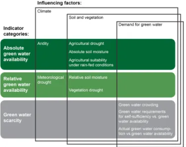
Figure 1.Conceptual diagram of indicator categories and the fac-tors that influence them.

3.1 Green water availability indicators

Indicators of green water availability fall apart in indicators that measure availability in an absolute sense or in terms of relative to normal conditions. These two categories are treated in the next two subsections. Descriptions of various specific green water availability indicators that fall in the two categories are included in Appendices A and B. The indi-cator abbreviations used in this section are defined in these appendices.

3.1.1 Absolute green water availability indicators Indicators in this category measure green water availability in a certain area (or location) and period (or moment) in an absolute sense. We find here indicators of aridity, agricultural drought, soil moisture and agricultural suitability, which are subsequently discussed in the following. Aridity indicators

are purely climatic, while the others are also influenced by the characteristics and management of the soil and vegeta-tion.

Aridity indicators

Aridity is seen as a permanent feature of a climate, consist-ing of low average annual precipitation and/or high evapo-ration rates, often resulting in low soil moisture availability (Pereira et al., 2002; Heim, 2002; Kallis, 2008). As such, one can say that an aridity map shows the preconditions for vege-tation (Falkenmark and Rockström, 2004). Aridity indicators are usually based on long-term average annual comparisons of precipitation versus potential evaporation, temperature or atmospheric saturation deficit, whereby the latter two were often used in the twentieth century as proxies for potential evaporation due to lack of data. They have been used for the classification of climates, specifically the characterization of (semi-)arid zones. Some more recently developed aridity in-dicators compare the actual rather than potential evaporation rate with precipitation (ER, HU-ER). These indicators reflect the actual availability of water at a given location (also from lateral fluxes) for meeting the evaporative demand of the at-mosphere.

(7)

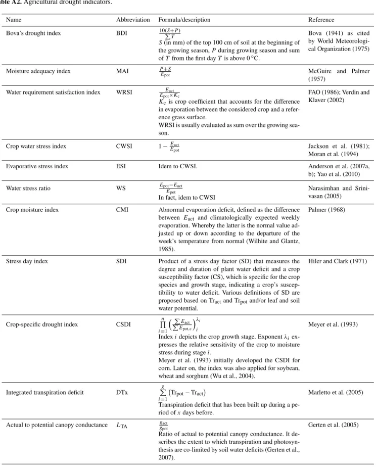
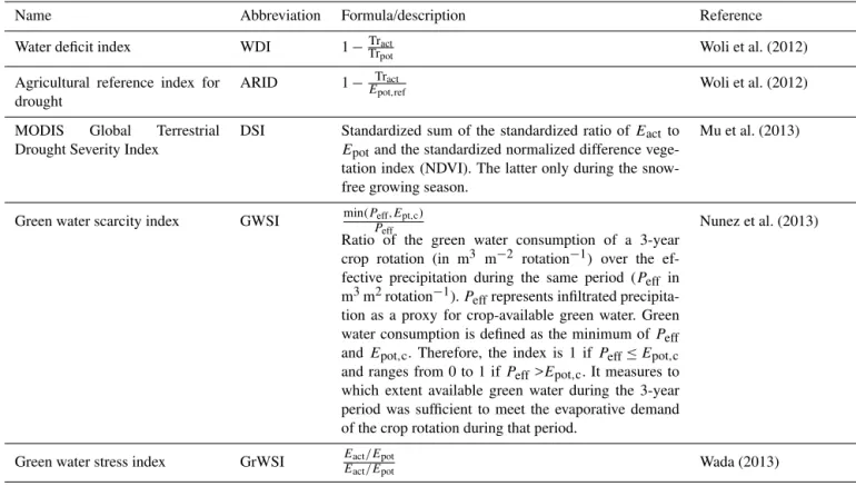
Agricultural drought indicators

According to the World Meteorological Organization (1975), agricultural drought indicators “indirectly express the de-gree to which growing plants have been adversely affected by an abnormal moisture deficiency”, which may be the re-sult of an unusually small moisture supply or an unusually large moisture demand (World Meteorological Organization, 1975). Formulated differently by Sivakumar (2011): “Agri-cultural drought depends on the crop evapotranspiration de-mand and the soil moisture availability to meet this dede-mand.” Therefore, the bulk of agricultural drought indicators mea-sures crop-available water compared to crop water needs for non-water limited growth (i.e. potential evaporation) and are usually applied on a daily, weekly, monthly or seasonal basis (Woli et al., 2012). Some indicators measure the plant water deficit more specifically by looking at the difference between actual and potential transpiration (e.g. DTx and WDI). Agri-cultural drought indicators can be influenced by soil manage-ment that affects the rates of infiltration and percolation and thus the water available to the crop.

Drought is typically a relative-to-normal phenomenon as will be discussed in Sect. 3.1.2. Agricultural drought indica-tors, which measure actual relative to potential evaporation, are relative indicators in another way, though. They do not compare actual with normal conditions. Instead, they com-pare moisture supply with a crop water demand in the ideal case of non-water limited growth. Therefore these indica-tors actually measure absolute green water availability (ac-tual evaporation), set against this crop water demand. In fact, these indicators say more about the demand for blue water (irrigation) to ensure non-water limited crop growth than they do about green water availability. Some indicators do some-how compare the actual to potential evaporation ratio with a multi-year average (or median) of this ratio and are thus in essence relative indicators according to our classification. Examples are the CMI, DSI and GrWSI and anomalies of the ESI and WS. Nevertheless, they are classified as agricul-tural drought indicators because they, like most of the others, measure actual to potential evaporation.

A note is required on the GWSI by Nunez et al. (2013) of which the name suggests that it is a green water scarcity indi-cator. Nevertheless, we classify it as an agricultural drought indicator, because it measures actual moisture supply ver-sus crop-specific reference evaporation, albeit on a larger timescale (3-year crop rotation) than most other agricultural drought indicators.

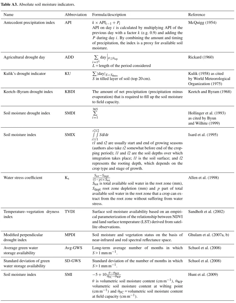
Absolute soil moisture indicators

Multiple indicators provide a measure of the absolute amount of soil moisture available at a given location and moment (or summed over a period), be it on the basis of field measure-ments (e.g. SMIX, SMI) and/or modelling of the soil wa-ter balance (e.g. Avg-GWS and SD-GWS) or remote

sens-ing data (e.g. TVDI, MPDI). They can be used for monitor-ing spatial and/or temporal variations in soil moisture avail-ability. Temporal analysis of soil moisture availability can warn for the onset of agricultural drought, or in contrast, the proneness to flash floods (Hunt et al., 2009). Several of these indicators have been introduced and applied as indica-tors of agricultural drought (e.g. ADD, SMDI, SMIX, SMI), analysing the correlation between soil moisture availability and crop yields. Therefore, they are typically calculated on intra-annual timescales.

It should be noted that the soil moisture can partially be blue – also under rain-fed conditions – due to capillary rise or natural flooding (Sect. 2.3). This note also applies to the other indicators that are not purely based on climatic factors (Fig. 1).

Agricultural suitability under rain-fed conditions Maps that classify land according to agricultural suitabil-ity under rain-fed conditions (green water only) are indirect measures of green water availability in the absolute sense. Up to date, two global studies have made such land suitabil-ity classifications for rain-fed crop production for climate-average temperature and precipitation conditions and taking into account crop characteristics, various soil parameters and terrain slope: GAEZ (IIASA/FAO, 2012) and GLUES (Zabel et al., 2014). The GAEZ study additionally considers various levels of agricultural input/management. Both studies clas-sify lands as not suitable, marginally suitable, moderately suitable or highly suitable. This classification shows where the climate, soil and topographic conditions are more or less suitable for agricultural production with green water only. In other words, where aridity maps show the preconditions for vegetation in general (Falkenmark and Rockström, 2004), these maps show the preconditions for rain-fed crop produc-tion, therein considering crop, soil and terrain parameters in addition to climate.

.2 Relative green water availability indicators

(8)

indicators are solely based on climatic variables. The other two subcategories are also affected by the soil and vegeta-tion and how they are managed. The three subcategories are sequentially discussed in the following.

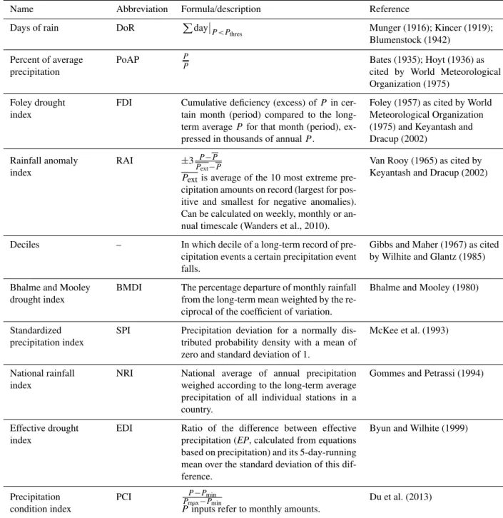
Meteorological drought indicators

Meteorological drought indicators fall apart in indicators that are solely based on precipitation (e.g. SPI) and those that consider both precipitation and potential evaporation (e.g. PDSI, RDI, SPEI). These indicators show whether there is relatively little precipitation or whether the normal balance between precipitation and evaporation is distorted. Unlike aridity indicators, which are generally based on long-term annual averages reflecting climate, these indicators capture variations in the weather. They are applied for monitoring the intensity, duration and spatial extent of droughts and deter-mining drought severity based on these characteristics. This is useful for recognizing droughts and comparing them with past drought, which serves as a basis for early warning sys-tems and decision-support tools.

Vegetation drought indicators

Vegetation drought indicators show the drought impact on vegetation by measuring the weather-related variations in greenness of vegetation. They reflect whether vegetation greenness is deviating from regular conditions. They can be used for studying the correlation between vegetation health and soil moisture availability, thermal conditions and crop yields (Kogan, 2001). Since the vegetation drought indica-tors we have identified are all based on remote sensing ob-servations, the indicators do not directly show whether devi-ations are caused by relatively dry weather (i.e. meteorologi-cal drought) or by other factors influencing vegetation growth (e.g. plant diseases or human interference such as pruning and clearing). Satellite-based vegetation drought indicators respond to subtle changes in vegetation canopy, which makes them suitable for early drought detection (Kogan, 2001). Relative soil moisture indicators

In contrast to the absolute soil moisture indicators discussed in Sect. 3.1.1, these indicators measure the moisture condi-tions at a given location relative to a normal condition. Iden-tified examples are the PZI, SMAI and SD. These indica-tors have similar uses as absolute soil moisture indicaindica-tors. They are also used to correlate soil moisture conditions to crop yields and are considered suitable for measuring agri-cultural droughts (Keyantash and Dracup, 2002; Narasimhan and Srinivasan, 2005).

3.2 Green water scarcity indicators

As put forward in Sect. 2, water scarcity pertains to a situa-tion with a high water demand compared to water

availabil-ity, which is experienced by a community (numerous people) within a certain geographic area (e.g. catchment or country) over a significant period of time (months or years). We can then define green water scarcity as the degree of competition over limited green water resources, whereby the demand for green water resources to sustain the production of a desirable level of biomass-based products within a certain geographic area is somehow compared to the available green water re-sources in space and time.

Since production of biomass-based products (food, fibres, biofuels, timber) generally takes place in cycles of 1 year (or more in case of perennials and forestry), this definition of green water scarcity incorporates the significant-period-of-time element in the imbalance between green water demand and availability. Furthermore, limited production of biomass-based products affects numerous people, both producers and consumers.

As opposed to the indicators discussed in Sect. 3.1, indi-cators of green water scarcity thus need to include a mea-sure of green water demand, associated with the production of biomass for human purposes, compared to green water availability. In other words, they should measure the green water demand related to crop production, grazing lands and forestry in relation to green water availability. Note that the term green water availability here refers to the part of the green water flow available for biomass production for human purposes (in space and time); it thus excludes green water flows that are effectively unavailable, for instance green wa-ter flows in unsuitable areas (e.g. because of steep slopes) or green water flows in cold parts of the year unsuitable for growth.

We distinguish three different options to measure green water scarcity conceptually:

1. green water crowding: per capita available green wa-ter resources in an area compared to a global average threshold representing the amount of green water re-quired to sustain a person’s standard consumption pat-tern of biomass-based products;

2. green water requirements for self-sufficiency versus green water availability: green water requirements for producing the consumed biomass-based products within a certain geographic area, assuming self-sufficiency within the geographic area, compared to the green water resources in the geographic area;

(9)

In Sect. 3.2.1 and 3.2.2, we discuss existing indicators that measure overall green–blue water scarcity and reflect on how these indicators could be adapted to measure green water scarcity specifically, according to above-mentioned options (1) and (2). In Sect. 3.2.3, we elaborate upon a third way of measuring green water scarcity that has yet to be brought into practice. The challenges for operationalization of these green water scarcity indicators are discussed in Sect. 3.2.4. Finally, in Sect. 3.2.5 we reflect on green water scarcity indi-cators versus indiindi-cators that measure overall green–blue wa-ter scarcity.

3.2.1 Green water crowding

Rockström et al. (2009) introduced a combined green–blue water shortage index, which compares the sum of green and blue water availability with a global average threshold of 1300 m3cap−1_yr−1_{. This threshold represents the green and} blue water requirements for sustaining a global average stan-dard diet. When green–blue water availability drops below the threshold, this indicates a shortage of green–blue wa-ter resources in the study area and reflects the area’s de-pendency on external water resources. The green–blue water shortage index is an indicator of water crowding, similar to Falkenmark’s blue-water-focussed water crowding indicator (Falkenmark et al., 1989).

Similar to the indicator by Rockström et al. (2009), an in-dicator of green water crowding could be defined as the per capita available green water resources in an area compared to a global average threshold representing the amount of green water required to sustain a person’s standard consumption pattern. We intentionally speak here of a consumption pat-tern, because green water is required not only to produce food, but also to produce other biomass-based products hu-mans consume, such as fibres, biofuels and forestry products. As such, the measure of green water requirements we pro-pose here is broader than the definition of a standard diet ac-cording to Rockström et al. (2009) (and Gerten et al., 2011; Kummu et al. 2014), which only pertains to water require-ments for food production.

Rockström et al. (2009) define green water availability as “the soil moisture available for productive vapour flows from agricultural land”. Technically, they calculate green water availability as actual evaporation from existing cropland and permanent pasture, reduced by a factor 0.85 that accounts for minimum evaporation losses that are unavoidable in agricul-tural systems (Rockström et al., 2009). This definition is de-pendent on the extent of agricultural land and excludes avail-able green water on lands that are currently uncultivated, but have potential to be used productively in a sustainable man-ner.

3.2.2 Green water requirements for self-sufficiency versus green water availability

Gerten et al. (2011) and Kummu et al. (2014) elaborated on the work by Rockström et al. (2009) by further developing and applying the overall green–blue water scarcity indica-tor. Instead of using a global average, Gerten et al. (2011) calculate the green–blue water requirements for sustaining a standard diet on the national level based on local crop water productivities and compare this with the sum of green and blue availability in each country of the world. The resulting green–blue water scarcity indicator, computed for each coun-try, is defined as the ratio between green–blue water avail-ability and green–blue water requirements for producing the standard diet. They define green water availability similar to Rockström et al. (2009), but a bit more conservative: they do not assume year-round evaporation from areas covered with their category of other crops that they parameterized as perennial grass, since this category includes non-food crops and crops that grow only during a part of the year (Gerten et al., 2011).

Whereas the studies by Rockström et al. (2009) and Gerten et al. (2011) are based on climate-averages, Kummu et al. (2014) apply the green–blue water scarcity indicator by Gerten et al. (2011) on a year-by-year basis to account for inter-annual climate variability on the scale of food produc-ing units, the scale at which demand for water and food is assumed to be managed according to the authors. Kummu et al. (2014) measure the frequency of years in which green– blue water availability falls short of green–blue water re-quirements, on which they base their classification of green– blue scarcity: no scarcity, occasional scarcity (subdivided in four levels) or chronic scarcity.

The green–blue water scarcity indicator shows the po-tential of a geographic area (e.g. country or food produc-ing unit) to reach food self-sufficiency and reflects its de-pendency on trade in agricultural commodities and associ-ated virtual water (Kummu et al., 2014). A similar indicator for green water could show an area’s green water demand (for self-sufficiency in biomass-based products, for sustain-ing the standard consumption pattern) compared to green wa-ter availability in the area. It would also reflect an area’s de-pendency on internal blue water resources and virtual water trade.

(10)

3.2.3 Actual green water consumption versus green water availability

The green water scarcity indicator by Hoekstra et al. (2011) compares the actual green water consumption in an area as-sociated with the actual biomass production pattern (hence considering virtual water trade as opposed to assuming self-sufficiency) with green water availability in the area. Green water scarcity is defined as the ratio of the total green water footprint in a catchment in a period (e.g. a year) over green water availability.

The sum of green water footprints equals all actual evap-oration (Eact)related to biomass production for human pur-poses (i.e. agriculture and forestry) excluding the part of the vapour flow that originates from blue water resources (irriga-tion). Note that for cases where land use is partly natural and partly for human production (e.g. a semi-natural production forest), the green water demand related to human production would need to be expressed as a fraction of the total green water flow. Methods to do so for a production forest are dis-cussed by van Oel and Hoekstra (2012). Green water avail-ability is defined as totalEactover the catchment minusEact from land reserved for natural vegetation (so-called environ-mental green water requirement) and minusEact from land that cannot be made productive, e.g. in areas or periods of the year that are unsuitable for crop growth (Hoekstra et al., 2011). In fact, green water availability defined like this, rep-resents the maximum sustainable green water footprint in the catchment and period under consideration. Hence, the green water scarcity ratio shows the extent to which the green wa-ter footprint has reached its maximum sustainable level. Of course, this definition can also be applied to other geograph-ical units than a catchment.

The definition of green water availability by Hoekstra et al. (2011) is more comprehensive than the one used by Rock-ström et al. (2009), Gerten et al. (2011) and Kummu et al. (2014). However, this is also the reason why the indica-tor has not been made operational yet. Difficulties remain in estimating the amount of land that needs to be reserved for nature and when and where the green water flow cannot be made productive (Hoekstra et al., 2011). These challenges are discussed in the following section.

Furthermore, the indicator does not deal with green wa-ter scarcity at a particular site as looked upon by Falken-mark et al. (2007) and FalkenFalken-mark (2013a). They describe green water scarcity as an issue of lower-than-potential plant-accessible water in the root zone and the occurrence of un-productive evaporation losses from the field, which results in lower yields than potentially achievable. First, blue water losses in the form of surface run-off and percolation decrease the plant-accessible water in the root zone (smaller green wa-ter flow) (Rockström and Falkenmark, 2000). Such losses are the result of a soil’s low infiltration capacity (e.g. soil crust-ing) and poor soil water holding capacity, but can be caused or aggravated by human action through soil mismanagement

(Falkenmark, 2013a). Second, low root/crop water uptake ca-pacity leads to unproductive evaporation losses (green water flow not entirely productive) (Rockström and Falkenmark, 2000). Transpiration is a productive form of green water use, contributing to biomass production, while other components of the evaporative flow are regarded as unproductive (Rock-ström and Falkenmark, 2000; Rock(Rock-ström, 2001; Rockstrom et al., 2007; Savenije, 2004). Rockstrom et al. (2007) express the productivity of green water use as the ratio of transpira-tion to evaporatranspira-tion. Rockström et al. (2009) call this the tran-spiration efficiency. This trantran-spiration efficiency is comple-mentary to the green water scarcity indicator by Hoekstra et al. (2011). A green water scarcity assessment based on both will give insight into theseverityof green water scarcity: ar-eas that are considered highly green–water scarce, but have a low transpiration efficiency, may have options to improve the latter and thereby yields, which may lower the green wa-ter scarcity.

3.2.4 Challenges for operationalization of green water scarcity indicators

Operationalization of green water scarcity indicators faces three major challenges, particularly regarding the quantifica-tion of green water availability.

First, the determination of which areas and periods of the year the green water flow can be used productively is not straightforward. Absolute green water availability indi-cators, in particular land classifications of agricultural suit-ability, can provide insight in the availability of green wa-ter in the spatial dimension. Relative green wawa-ter availabil-ity indicators can enrich the picture by showing which areas are prone to large inter- and intra-annual variations in green water availability, making these areas less suitable for (cer-tain types of) biomass production. To estimate which part of the green water flow can be used productively in time, ad-vanced crop growth models (like APSIM, McCown et al., 1995 and Holzworth et al., 2014; AquaCrop, Steduto et al., 2009; CropSyst, Stöckle et al., 2003; EPIC, Jones et al., 1991 or SWAP/WOFOST, van Dam et al., 2008) can be used to simulate water-limited yields and actual evaporation for var-ious cropping periods and different types of soil, crop and agricultural water management (e.g. adding blue water in the form of deficit irrigation during a dry spell, might make it possible for the crop to survive and use the green water flow later in the year productively).

Second, estimating green water consumption of forestry is difficult, because it entails separation of production forest evaporation into green and blue parts. This is problematic, because trees generally root so deep that, by means of capil-lary rise, they directly take up water from groundwater (blue) in addition to the soil moisture (green) (Hoekstra, 2013).

(11)

environmen-tal flow requirements for blue water. Key here is the iden-tification of areas that need to be reserved for nature and biodiversity conservation. It is known that the current net-work of protected areas is insufficient to conserve biodiver-sity (Rodrigues et al., 2004a, b; Venter et al., 2014; Butchart et al., 2015) and that attention should be paid to conserva-tion of biodiversity in producconserva-tion landscapes that are shared with humans (Baudron and Giller, 2014). The 11th Aichi Biodiversity Target is to expand the protected area network, which currently has a terrestrial coverage of about 14.6 % (Butchart et al., 2015), to at least 17 % terrestrial coverage by 2020 (Convention on Biological Diversity, 2010). How-ever, to properly assess the limitations to green water avail-ability, spatially explicit information on the additional areas to be preserved is required. The best-available data regard-ing this are recently published work by Montesino Pouzols et al. (2014). These authors have mapped global and national priority areas for expansion of the protected area network on 0.2 degree spatial resolution and assessed associated conser-vation gains (Montesino Pouzols et al., 2014; Brooks, 2014). 3.2.5 Measuring green water scarcity versus overall

green–blue water scarcity

In Sect. 3.2.1 and 3.2.2, we mentioned a few indicators that measure overall green–blue water scarcity (Rockström et al., 2009; Gerten et al., 2011; Kummu et al., 2014). Whereas use-ful for getting an overall picture of water scarcity, a disadvan-tage of these indicators is that a high degree of green water scarcity can be masked by a low degree of blue water scarcity and vice versa. Imagine for example a river basin where nearly all land is in use and natural forest is under pressure by conversion to cropland (high degree of green water scarcity), while there is enough blue water available to irrigate crop-lands if necessary (low degree of blue water scarcity). Mea-suring increasing green water scarcity could be relevant, for instance, for the Amazon basin in South America, where in-creasingly natural forest and associated green water flows are turned into use and competition is essentially about land and associated green water resources, while blue water resources are abundant and blue water scarcity is low. Therefore, for studying green water scarcity, an indicator specifically com-paring green water demand and green water availability can be more appropriate.

4 Conclusions and future research

In this paper we have reviewed and classified around 80 indi-cators of green water availability and scarcity. This list of in-dicators is extensive, but not exhaustive. Nevertheless, we are confident to have identified the most widely used and cited indicators.

The number of green water availability indicators by far outnumbers the existing green water scarcity indicators. This reflects that the concept of green water scarcity is still largely unexplored. Indicators of overall green–blue water crowding and scarcity have been developed by Rockström et al. (2009), Gerten et al. (2011) and Kummu et al. (2014). These have po-tential to be tailored to measure green water crowding and green water requirements for self-sufficiency versus green water availability. The green water scarcity indicator by Hoekstra et al. (2011) measures actual green water consump-tion versus green water availability, but has not yet been oper-ationalized due to several challenges discussed in Sect. 3.2.4. The biggest challenge is to determine which part of the green water flow can be made productive in space and time. Ap-plication of both absolute and relative green water availabil-ity indicators will provide insight into where the green wa-ter flow can be made productive for human purposes. Sim-ulations with crop growth models for different management strategies can be used to assess during which parts of the year the green water flow can be made productive.

Future research should be aimed at overcoming these chal-lenges to make the green water scarcity indicators discussed in this paper operational. We also encourage the development of additional definitions of green water scarcity indicators to the ones discussed here. The conceptual definition of green water scarcity we introduced in Sect. 3.2 can be a starting point for this.

(12)

Appendix A: Absolute green water availability indicators

(13)

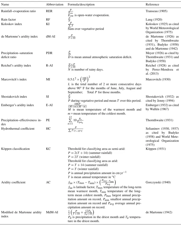
Table A1.Aridity indicators.

Name Abbreviation Formula/description Reference

Rainfall–evaporation ratio RER _EP

ow

Eowis open-water evaporation.

Transeau (1905)

Rain factor RF P_T Lang (1920)

Koloskov index KI PP

T

Sum over vegetative period

Koloskov (1925) as cited by World Meteorological Organization (1975)

de Martonne’s aridity index dM-AI _T₊P₁₀ de Martonne (1926) as

cited by Thornthwaite (1931), Budyko (1958) and de Martonne (1942) Precipitation–saturation

deficit ratio

PDR _DP

Dis mean annual atmospheric saturation deficit.

Meyer (1926) as cited by Thornthwaite (1931) and Budyko (1958)

Reichel’s aridity index R-AI _TN₊×₁₀P

Nis number of rainy days.

Reichel (1928) as cited

by Perez-Mendoza et

al. (2013)

Marcovitch’s index MI 0.5L2×

100

P

2

Lis the total number of 2 or more consecutive days above 90◦F for the months of June, July, August and September; TotalP for those months.

Marcovitch (1930)

Shostakovich index SI P_T

Pduring vegetative period and meanT over this period.

Shostakovich (1932) as cited by Jenny (1994)

Emberger’s aridity index E-AI _(M₊100_m)(MP₋_m)

M is mean temperature of the warmest month and

m= mean temperature of the coldest month.

Emberger (1932) as cited by Wallén (1967)

Precipitation–effectiveness in-dex

PE

12 P

n=1

10 Pn

Epot_n Thornthwaite (1931)

Hydrothermal coefficient HC P P

T|T >10◦C Selianinov (1930, 1937)

as cited by Budyko

(1958) and World Mete-orological Organization (1975)

Köppen classification KC Threshold for classifying area as semi-arid:

P=2(T+14)(summer rainfall)

P=2T (winter rainfall)

Threshold for classifying area as arid:

P=T+14 (summer rainfall)

P=T (winter rainfall)

Pis annual precipitation amount in cm yr−1

T is mean annual temperature in◦C

Köppen (1931)

Aridity coefficient AC flat×(Tmax−Tmin)×

Pmax−Pmin

Pavg

flatis latitude factor,Tmaxtemperature of the long-term

mean warmest month,T_min temperature of the long-term mean coldest month,Pmaxlargest annual precip-itation amount on record,Pminsmallest annual

precip-itation amount on record andPavgaverage annual pre-cipitation amount on record.

Gorczynski (1940)

Modified de Martonne aridity index

MdM-AI 1₂_T₊P₁₀+ 12Pd

Td+10

Pdis precipitation in the driest month andTd

tempera-ture in the driest month.

(14)

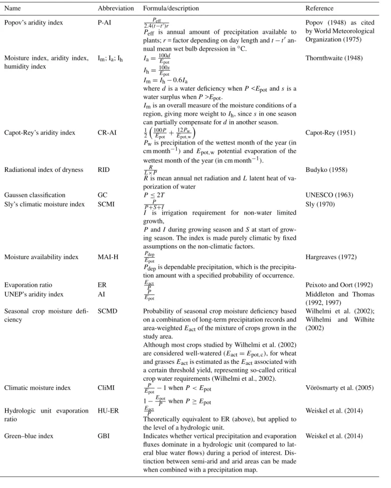
Table A1.Continued.

Popov’s aridity index P-AI Peff

2.4(t−t′_)r

P_eff is annual amount of precipitation available to plants;r= factor depending on day length andt−t′ an-nual mean wet bulb depression in◦C.

Popov (1948) as cited by World Meteorological Organization (1975)

Moisture index, aridity index, humidity index

Im; Ia; Ih Ia=100_E_potd Ih=100Epots Im=Ih−0.6Ia

wheredis a water deficiency whenP <Epotandsis a

water surplus whenP >Epot.

Imis an overall measure of the moisture conditions of a region, giving more weight toIh, sincesin one season

can partially compensate fordin another season.

Thornthwaite (1948)

Capot-Rey’s aridity index CR-AI 1₂100_E P

pot + 12Pw

Epot,w

Pwis precipitation of the wettest month of the year (in

cm month−1) and Epot,w potential evaporation of the

wettest month of the year (in cm month−1).

Capot-Rey (1951)

Radiational index of dryness RID _L_×R_P

Ris mean annual net radiation andLlatent heat of va-porization of water

Budyko (1958)

Gaussen classification GC P≤2T UNESCO (1963)

Sly’s climatic moisture index SCMI _P₊P_S₊_I

I is irrigation requirement for non-water limited

growth,

P andIduring growing season andSat start of grow-ing season. The index is made purely climatic by fixed assumptions on the non-climatic factors.

Sly (1970)

Moisture availability index MAI-H P_Edep

pot

Pdepis dependable precipitation, which is the

precipita-tion amount with a specified probability of occurrence.

Hargreaves (1972)

Evaporation ratio ER Eact

P Peixoto and Oort (1992)

UNEP’s aridity index AI _EP

pot Middleton and Thomas

(1992, 1997) Seasonal crop moisture

defi-ciency

SCMD Probability of seasonal crop moisture deficiency based

on a combination of long-term precipitation records and area-weightedEactof the mixture of crops grown in the study area.

Although most crops studied by Wilhelmi et al. (2002) are considered well-watered (Eact=Epot,c), for wheat

and grassesEactis estimated as theEactassociated with a certain threshold yield, representing so-called critical crop water requirements (Wilhelmi et al., 2002).

Wilhelmi et al. (2002);

Wilhelmi and Wilhite

(2002)

Climatic moisture index CliMI _EP

pot−1 whenP < Epot

1−E_Ppot whenP ≥Epot

Vörösmarty et al. (2005)

Hydrologic unit evaporation ratio

HU-ER Eact

P

Theoretically equivalent to ER (above), but applied to the level of a hydrologic unit.

Weiskel et al. (2014)

Green–blue index GBI Indicates whether vertical precipitation and evaporation

fluxes dominate in a hydrologic unit (compared to lat-eral blue water flows) during a period of interest. Dis-tinction between semi-arid and arid areas can be made when combined with a precipitation map.

(15)

Table A2.Agricultural drought indicators.

Bova’s drought index BDI 10(SP+P ) T

S(in mm) of the top 100 cm of soil at the beginning of the growing season,Pduring growing season and sum ofTfrom the first dayTis above 0◦C.

Bova (1941) as cited by World Meteorologi-cal Organization (1975)

Moisture adequacy index MAI P_E+S

pot McGuire and Palmer

(1957)

Water requirement satisfaction index WRSI Eact

Epot×Kc

Kcis crop coefficient that accounts for the difference in evaporation between the considered crop and a refer-ence grass surface.

WRSI is usually evaluated as sum over the growing sea-son.

FAO (1986); Verdin and Klaver (2002)

Crop water stress index CWSI 1−Eact

Epot Jackson et al. (1981);

Moran et al. (1994)

Evaporative stress index ESI Idem to CWSI. Anderson et al. (2007a, b); Yao et al. (2010)

Water stress ratio WS Epot_E−Eact pot

In fact, idem to CWSI

Narasimhan and Srini-vasan (2005)

Crop moisture index CMI Abnormal evaporation deficit, defined as the difference between Eact and climatologically expected weekly evaporation. Whereby the latter is the normal value ad-justed up or down according to the departure of the week’s temperature from normal (Wilhite and Glantz, 1985).

Palmer (1968)

Stress day index SDI Product of a stress day factor (SD) that measures the degree and duration of plant water deficit and a crop susceptibility factor (CS), which is specific for the crop species and growth stage, indicating a crop’s suscep-tibility to water deficit. Various definitions of SD are proposed based on Tractand Trpotand/or leaf and soil water potential.

Hiler and Clark (1971)

Crop-specific drought index CSDI

n Q i=1

P Eact

P Epot,c

λi

i

Indexidepicts the crop growth stage. Exponentλi ex-presses the relative sensitivity of the crop to moisture stress during stagei.

Meyer et al. (1993) initially developed the CSDI for corn. Later on, the index was also applied for soybean, wheat and sorghum (Wu et al., 2004).

Meyer et al. (1993)

Integrated transpiration deficit DTx

χ P i=1

Trpot−Tract

Transpiration deficit that has been built up during a pe-riod ofxdays before.

Marletto et al. (2005)

Actual to potential canopy conductance LTA ggactpot

Ratio of actual to potential canopy conductance. It de-scribes the extent to which transpiration and photosyn-thesis are co-limited by soil water deficits (Gerten et al., 2007).

(16)

Table A2.Continued.

Water deficit index WDI 1− Tract

Trpot Woli et al. (2012)

Agricultural reference index for drought

ARID 1− Tract

Epot,ref Woli et al. (2012)

MODIS Global Terrestrial

Drought Severity Index

DSI Standardized sum of the standardized ratio ofEact to

Epotand the standardized normalized difference

vege-tation index (NDVI). The latter only during the snow-free growing season.

Mu et al. (2013)

Green water scarcity index GWSI min(P_Peff,Ept,c)

eff

Ratio of the green water consumption of a 3-year crop rotation (in m3 m−2 rotation−1) over the ef-fective precipitation during the same period (Peff in

m3m2rotation−1).Peffrepresents infiltrated

precipita-tion as a proxy for crop-available green water. Green water consumption is defined as the minimum ofPeff

andEpot,c. Therefore, the index is 1 ifPeff≤Epot,c

and ranges from 0 to 1 ifP_eff >Epot,c. It measures to

which extent available green water during the 3-year period was sufficient to meet the evaporative demand of the crop rotation during that period.

Nunez et al. (2013)

Green water stress index GrWSI E_Eact/Epot

(17)

Table A3.Absolute soil moisture indicators.

Antecedent precipitation index API k×API_i₋₁+P_i

API on dayiis calculated by multiplying API of the previous day with a factork(e.g. 0.9) and adding the

P during dayi. By combining the amount and timing of precipitation, the index is a proxy for available soil moisture.

McQuigg (1954)

Agricultural drought day ADD P

i=1L day

θ≤θwp

L= length of the period considered

Rickard (1960)

Kulik’s drought indicator KU P_|

day|_S<S thres

Sin tilled layer of soil (top 20 cm).

Kulik (1958) as cited by World Meteorological Organization (1975)

Keetch–Byram drought index KBDI The amount of net precipitation (precipitation minus

evaporation) that is required to fill up the soil moisture to field capacity.

Keetch and Byram (1968)

Soil moisture drought index SMDI

365 P

i=1

Hollinger et al. (1993) as cited by Byun and Wilhite (1999)

Soil moisture index SMIX

t2 R

t1

l2 R

l1 Sdldt

t1andt2are usually start and end of growing seasons (authors also taket2somewhat before end of the crop-ping period);l1andl2are the soil depths over which integration takes place;l1is the soil surface; andl2

represents the rooting depth, which depends on the crop type and stage of growth.

Isard et al. (1995)

Water stress coefficient Ks ₍S₁tot₋_p)−S_×depl_S tot

Stotis total available soil water in the root zone (mm),

Sdepl root zone depletion (mm) and p part of total

available soil water in the root zone that a crop can ex-tract from the root zone without suffering from water stress.

Allen et al. (1998)

Temperature–vegetation dryness index

TVDI Surface soil moisture availability based on an

empiri-cal parameterization of the relationship between NDVI and land surface temperature (LST) derived from satel-lite observations.

Sandholt et al. (2002)

Modified perpendicular drought index

MPDI Soil moisture and vegetation status on the basis of

near-infrared and red spectral reflectance space.

Ghulam et al. (2007a, b)

Average green water storage availability

Avg-GWS Long-term average number of months in which

S> 1 mm m−1.

Schuol et al. (2008)

Standard deviation of green water storage availability

SD-GWS Standard deviation of the number of months in which

S> 1 mm m−1.

Schuol et al. (2008)

Soil moisture index SMI −5+10 θ−θWP

θFC−θWP

θis volumetric soil moisture content (cm m−1),θWP

volumetric soil moisture content at wilting point (cm m−1)andθFC= volumetric soil moisture content

at field capacity (cm m−1).

(18)

Table A4.Agricultural suitability under rain-fed conditions.

GAEZ crop-specific suitability under rain-fed conditions

GAEZ Crop-specific suitability under rain-fed conditions is

based on estimates of agro-ecologically attainable yields. First, agro-climatically attainable yields are determined based on a water balance approach that calculatesEactand additionally considers crop water

requirements and a crop’s sensitivity to water stress during the various stages of growth to calculate a yield reduction factor due to water limitations. Sec-ond, agro-climatically attainable yields are further re-duced by agro-edaphic constraints.

IIASA/FAO (2012)

GLUES crop-specific suitabil-ity under rain-fed conditions

GLUES Crop-specific suitability under rain-fed conditions is

based on a fuzzy logic approach with crop-specific membership functions for climatic, soil and topo-graphic conditions. Yield estimates are not provided by the GLUES methodology.

(19)

(20)

Table B1.Meteorological drought indicators based on precipitation only.

Days of rain DoR P

day_{P <P}

thres Munger (1916); Kincer (1919);

Blumenstock (1942)

Percent of average precipitation

PoAP P

P Bates (1935); Hoyt (1936) as

cited by World Meteorological Organization (1975)

Foley drought index

FDI Cumulative deficiency (excess) ofP in

cer-tain month (period) compared to the long-term averageP for that month (period), ex-pressed in thousands of annualP.

Foley (1957) as cited by World Meteorological Organization (1975) and Keyantash and Dracup (2002)

Rainfall anomaly index

RAI ±3 P−P

Pext−P

Pextis average of the 10 most extreme pre-cipitation amounts on record (largest for pos-itive and smallest for negative anomalies). Can be calculated on weekly, monthly or an-nual timescale (Wanders et al., 2010).

Van Rooy (1965) as cited by Keyantash and Dracup (2002)

Deciles – In which decile of a long-term record of

pre-cipitation events a certain prepre-cipitation event falls.

Gibbs and Maher (1967) as cited by Wilhite and Glantz (1985)

Bhalme and Mooley drought index

BMDI The percentage departure of monthly rainfall

from the long-term mean weighted by the re-ciprocal of the coefficient of variation.

Bhalme and Mooley (1980)

Standardized precipitation index

SPI Precipitation deviation for a normally

dis-tributed probability density with a mean of zero and standard deviation of 1.

McKee et al. (1993)

National rainfall index

NRI National average of annual precipitation

weighed according to the long-term average precipitation of all individual stations in a country.

Gommes and Petrassi (1994)

Effective drought index

EDI Ratio of the difference between effective

precipitation (EP, calculated from equations based on precipitation) and its 5-day-running mean over the standard deviation of this dif-ference.

Byun and Wilhite (1999)

Precipitation condition index

PCI P−Pmin

Pmax−Pmin

P inputs refer to monthly amounts.

(21)

Table B2.Meteorological drought indicators based on precipitation and a measure of potential evaporation.

Palmer drought severity index PDSI Accumulated weighted

dif-ferences between actual

precipitation and precipitation

requirement of evaporation

(Wilhite and Glantz, 1985).

Palmer (1965); Alley (1984)

Reconnaissance drought index RDI Standardized ratio of P to

Epot based on a log-normal

distribution.

Tsakiris and Vangelis (2005); Tsakiris et al. (2007)

Standardized precipitation evapotranspiration index

SPEI Standardized difference

be-tweenP andEpotbased on a

log-logistic distribution.

Vicente-Serrano et al. (2009)

Water surplus variability index WSVI Standardized difference

be-tweenP andEpot,refbased on

a logistic distribution.

Gocic and Trajkovic (2014)

Table B3.Vegetation drought indicators.

Normalized difference vegetation index anomaly

NDVIA NDVI−NDVI Tucker (1979);

Myneni et al. (1998)

Vegetation condition index VCI NDVI−NDVImin

NDVImax−NDVImin

NDVImin is multi-year minimum of

smoothed weekly NDVI and NDVImax

multi-year maximum of smoothed weekly NDVI

Kogan (1990, 1995)

Vegetation health index VHI a·VCI+b·TCI

a is coefficient quantifying share of VCI contribution in the combined condition, b

coefficient quantifying share of TCI contri-bution in the combined condition, TCI Tem-perature Condition Index and VCI Vegeta-tion CondiVegeta-tion Index

Kogan (2001)

Standardized vegetation index SVI NDVI deviation for a normally distributed

probability density with a mean of zero and standard deviation of 1.

Peters et al. (2002)

Normalized difference water index anomaly

NDWIA Adaptation of NDVI (Gao, 1996) compared

to its multi-year mean.

Gu et al. (2007)

Enhanced vegetation index anomaly

EVIA EVI anomaly. EVI is an improvement over

NDVI, which keeps sensitivity over densely vegetated areas (Huete et al., 1994).

Saleska et al. (2007)