The Effect of Single Recombination Events on Coalescent
Tree Height and Shape
Luca Ferretti1,2, Filippo Disanto1, Thomas Wiehe1*
1Institut fu¨r Genetik, Universita¨t zu Ko¨ln, Ko¨ln, Germany,2Center for Research in AgriGenomics, Barcelona, Spain
Abstract
The coalescent with recombination is a fundamental model to describe the genealogical history of DNA sequence samples from recombining organisms. Considering recombination as a process which acts along genomes and which creates sequence segments with shared ancestry, we study the influence of single recombination events upon tree characteristics of the coalescent. We focus on properties such as tree height and tree balance and quantify analytically the changes in these quantities incurred by recombination in terms of probability distributions. We find that changes in tree topology are often relatively mild under conditions of neutral evolution, while changes in tree height are on average quite large. Our results add to a quantitative understanding of the spatial coalescent and provide the neutral reference to which the impact by other evolutionary scenarios, for instance tree distortion by selective sweeps, can be compared.
Citation:Ferretti L, Disanto F, Wiehe T (2013) The Effect of Single Recombination Events on Coalescent Tree Height and Shape. PLoS ONE 8(4): e60123. doi:10.1371/journal.pone.0060123
Editor:Nadia Singh, North Carolina State University, United States of America ReceivedNovember 15, 2012;AcceptedFebruary 21, 2013;PublishedApril 8, 2013
Copyright:ß2013 Ferretti et al. This is an open-access article distributed under the terms of the Creative Commons Attribution License, which permits unrestricted use, distribution, and reproduction in any medium, provided the original author and source are credited.
Funding:This work was supported by grants from the German Research Foundation (DFG-SFB680 ) to TW, grant AGL2010-14822 (MICINN,
Competing Interests:The authors have declared that no competing interests exist. * E-mail: [email protected]
Introduction
Coalescent theory is a central part of modern population genetics [1–3]. It constitutes the basis of genealogical models, of statistical tests of the neutral evolution hypothesis [4] as well as of many simulation tools [5–7]. Besides application in population genetics, coalescent models and their various generalizations became an object of study in their own right in probability, graph theory and combinatorics [8–12].
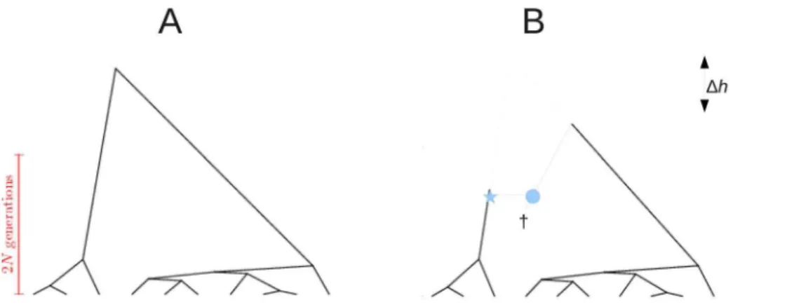
The classical coalescent is a binary, rooted, unordered tree with a fixed numbernof leafs. The latter is also called the sizeof the tree (Figure 1A). Such a tree can be interpreted as the genealogical history of a sample of DNA sequences, where mergers (‘‘coales-cents’’) of two lineages represent events of common ancestry. Thus, coalescent trees are naturally fitted with a time scale and for this reason they are sometimes calledlabelled histories. A biologically important generalization of the simple case is the coalescent with recombination. Recombination is a process by which two DNA sequences reciprocally exchange genetic material. In the coales-cent framework this translates into lineage splits (Figure 1B). A split represents the un-coupling of the genealogical history of two sequence fragments. The ancestral recombination graph (ARG) [13] is a model to integrate such lineage splits into coalescent trees. Each sequence positionxalong the chromosome is associated with a coalescent treeTx, which is the marginal tree of the ARG at positionx. Depending on the rate of recombination, chromosomes are divided into smaller or larger sequence fragments fi (‘‘haplotype block’’) in such a way that all positions within a fragment are free of recombination and therefore have the same marginal treeTf.
The spatial coalescent is the sequence(Tfi)iof coalescent trees along a sample of recombining chromosomes. Study of the spatial coalescent is of prominent interest in population genomics, since it contains information about the demographic and evolutionary history of a population. For instance, it has lately been used to infer demographic parameters in non-African human [14]. Unfortunately, the spatial coalescent is not a simple Markov process [15], complicating its probabilistic analysis and leaving many open problems to be addressed.
Here, we investigate the impact of single recombination events upon some measures of tree topology and shape. Bytopology we mean the branching pattern of a tree; by shape we mean its topology and branch lengths. In particular, we ask how recombination affects tree height and tree (im-)balance. The latter is measured by the difference in size of the left and right subtrees emerging from the root or any internal node. Depending on when and where a recombination event occurs, the effect on altering tree structure may be drastic, mild or completely silent. Informally, drastic events are those which lead to a large change of tree height or balance. These are events which typically involve splits by recombination of the branches emerging from the root of the tree. As such they may strongly affect the genealogical structure of haplotypes. Identifying and characterizing these events is very informative for population genetic inference. Mild events are typically those which occur along very recent branches, close to the leafs of the tree. They do not, or only mildly, affect haplotype structure and mutation frequency spectrum. Interestingly, there is a non-negligible portion of recombination events which do not alter tree topology, i.e. the branching pattern. We call these events
silent. Sometimes, also the branch lengths remain unchanged; we call these eventshidden(Figure 2).
and DFG-SPP1590
Spain) to Miguel Perez-Enciso and by a Consolider Grant from the Spanish Ministry of Research, CSD2007- 00036 ‘‘Centre for Research in Agrigenomics.’’ LF
data collection, and analysis, decision to publish, or preparation of the manuscript.
Our goals are to formalize these concepts, to characterize in more detail the effect of single recombination events upon tree shape and to quantify the relative frequencies of drastic, mild and silent events. We explicitly calculate the probabilities of changes in height or root balance induced by a single recombination event. Our results are based on the assumption of a standard neutral model of constant population size. This means that for each coalescent event two lineages are chosen at random to merge. Further, the timing of events is exponentially distributed with a rate which, after re-scaling by population sizeN, depends only on the number of lineages at a given time.
In Results Section (a), we define a probability density for the trees in the spatial coalescent and we explain the difference between pointwise marginal treesTx, evaluated at every basepair xof the DNA sequences, and the marginal treesTf, evaluated at every fragment f. We derive a simple relation between the densities of Tx and Tf. In Section (b) we analyze the recombination events which lead to height-changes and derive their probabilities. In Section (c) we quantify the concept of root imbalance, called V, and derive the first-order transition probabilities under single recombination events. We focus on events which produce unbalanced trees and, at the same time, lead to an increase of tree height. This type of events is of particular interest for the analysis of biological data. Their effect on the mutation frequency spectrum and on haplotype structure is the basis of tests to reject the neutral evolution hypothesis (e.g., [16– 18]). Therefore, for bench-marking it is highly interesting to know how often such events occur under purely neutral conditions, but it is not the goal of this paper to devise another neutrality test. Then, we generalize the results regarding the tree topology parameterV and derive the transition probability for arbitrary types of recombination events. Using this, we calculate the run-length distribution of V along recombining chromosomes. Finally, in Section 0.4, we calculate the average proportion of hidden recombination events and derive its limiting behavior for large sample sizes.
We remind the reader that the spatial coalescent is a non-Markovian process and not completely determined by transitions of any finite order. However, it is a homogeneous process. Therefore, first-order transition probabilities are well-defined and independent of the position in the sequence. Here, we compute first order probabilities for single recombination events from one
tree to the next, averaging over all trees of the ARG which are not directly involved in the recombination event considered. There-fore, our results hold for the spatial coalescent as described by the ARG [13]. In fact, the ARG is the model which is underlying all our calculations.
Results
(a) Tree Distribution and Recombination
We consider a sample of n ‘‘chromosomes’’ from a diploid panmictic population of constant sizeN. Without recombination, the genealogical history for these chromosomes is described by the classical coalescent process [1,2]. The set of all possible coalescent trees of size n is a product Rn{1
z 6Ln, where R n{1
z contains positive real waiting times ofn{1independent coalescent events and the discrete set Ln represents the set of all possible tree topologies. For our purposes here it is more convenient to consider labelled coalescent trees: this means that not only the internal nodes are ordered but also the leafs carry leaf labels. Hence [19] (see also http://oeis.org/A006472), the cardinality ofLnis
DLnD~n!(n{1)!
2n{1 : ð1Þ
Furthermore, all trees in Ln have the same probability 2n{1
n!(n{1)!, when they are generated under the standard coalescent process [20]. The waiting timestkfor a coalescent event, givenk lineages, are exponentially distributed with mean 1=k(k{1). Time runs backward from the leafs to the root of the tree and is measured in units of the coalescent, i.e. time is scaled by four times the population size. Therefore, Rn{z 16Ln can be regarded as being equipped with a probability mass function which factorizes into a probability densitypk(tk) for each waiting time (2ƒkƒn) and the discrete probability for the topologyP(top). For treesTin the above sense, we denote the resulting probability ‘density’ by
p(c)(T)~6nk~2pk(tk)|P(top)(T)
and we have
Figure 1. Example coalescent trees.A: Tree of sizen~10generated under the coalescent process. They-axis represents a time scale, with leafs at the ‘present’, and the root in the ‘past’. Starting from the present and going backwards in time, coalescent events are exponentially distributed with a parameter depending on population size (2N) and the number of lineages at any given point in time. B: Recombination is a prune (asterisk) and re-graft (circle) event: a lineage splits and merges onto another lineage which exists in the population at the time of recombination. This lineage does not need to extend to the present, and it may have become extinct from the entire population (cross). Recombination has changed the height of the coalescent tree with respect to the tree in panel A (Dh), but has not changed root imbalance: for both treesV~3.
p(c)(T)~ 2n {1
n!(n{1)! P n
k~2k(k
{1)e{k(k{1)tk(T), ð2Þ
wheretk(T)is the time interval during which the coalescent treeT hasklineages.
Modeling recombination as an ARG [13], there are two processes to be considered: coalescence and recombination. Given k independent lineages, in the coalescent process two lineages merge into a single one with ratek(k{1). In the recombination process, a single lineage splits into two with rate krL, where
r~4Nr denotes the population recombination rate, r is the recombination rate per base and L is the finite length of the sequence. After a recombinational split the two ancestral lineages correspond to different sequence fragments, left and right of the point of recombination. This point is chosen uniformly along the sequence of length L. We assume that r is small, so multiple recombination events in the same position are negligible.
Given a tree T(x) in position x, the length before the first recombination event downstream (or upstream) ofxis geometri-cally distributed with parameterrl(T), wherel(T)represents the total length of the tree. Since r is small, it can be safely approximated by an exponential distribution with the same parameterrl(T).
Recombination events may change the shape of the tree. The local tree at positionxin the genome may differ from the local tree at positionydue to recombination. Moving along the genome, we consider two different sequences of trees: the sequence Sx~fT(x1),T(x2),. . .gof local trees for all positions x1,x2,. . ., and the sequenceSf~fT(f1),T(f2),. . .gof local trees which are separated by asinglerecombination event (Figure 3). Note that a tree inSf can span several base positions, as the typical length 1=rl(Tf) of the fragment f is greater than 1. Also, note that consecutive trees in Sf need not be different. This occurs when fragments are separated by hidden recombination events.
The standard coalescent without recombination is recovered when looking at the tree for a single positionx in the sequence, ignoring all other trees. Neither the rate of coalescent events nor the choice of coalescing lineages in this tree are influenced by ancestral lineages at other positions. The local tree T(x)at any position x is therefore a standard coalescent tree without recombination [21] and the marginal density of a tree in position x of the ARG is identical to p(c)(T); i.e., picking the tree in
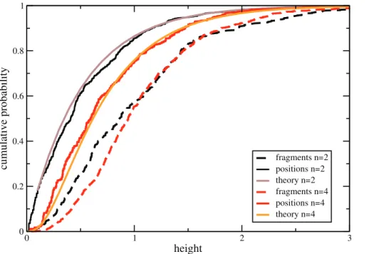
positionxfrom a random sequenceSxis equivalent to generating one from the standard coalescent process without recombination. On the other hand, picking a tree from a random sequenceSf results in a different distribution. The reason is that short trees recombine less, therefore they tend to span larger regions and to be under-represented in Sf compared to Sx, as illustrated in Figures 4 and 5.
In fact, the two distributions differ by weights which are proportional to the lengthLf of the fragments spanned by each tree. Since in the limit of large sequences the average length is E(Lf(T))~1=(rl(T)), we havep(c)(T)!p(r)(T)=l(T). Therefore, for large sequences, the tree density after a random recombination event is given by
p(r)(T)~l(T)
Ec(l)
p(c)(T) , ð3Þ
wherel(T) denotes the total length of the tree. For the standard neutral model, Ec(l)~an~Pn
{1
i~11=i. Note that the two distri-butions differ only in their weights of branch lengths, but not with respect to topology.
The argument leading to eq (3) can be made rigorous under the assumption of infinitely long chromosomes, using the fact that the coalescent with recombination is an ergodic process [22] (see Text S1, Supporting Information eqs (1)–(3)). As a check of eq (3), we show thatp(r)(T)is invariant under a single recombination event. Let Px(T’DT) be the transition density from tree T in a given positionxto treeT’in positionxz1, andPr(T’DT)the transition density from treeTto treeT’obtained by a single recombination event. Since the marginal density p(c)(T) is the same for every position, we have
p(c)(T’)~X T
Px(T’DT)p(c)(T) ð4Þ
independent of the recombination rate. For small recombination rates and at first order in r, we have Px(T’DT)~(1{rl(T))dT’,Tzrl(T)Pr(T’DT). Substituting this into (4) gives
l(T’)p(c)(T’)~X T
Pr(T’DT)l(T)p(c)(T): ð5Þ
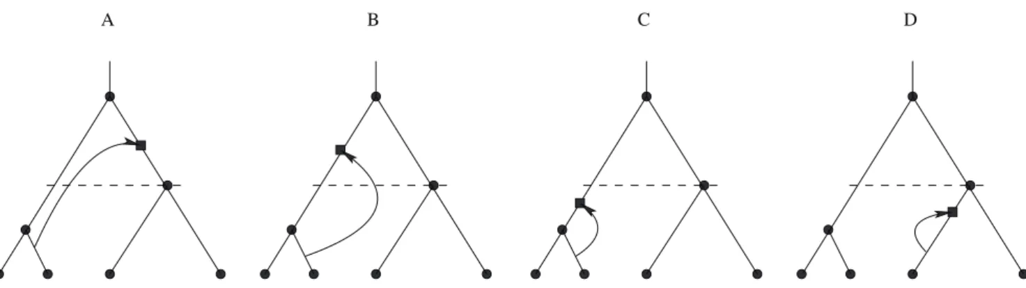
Figure 2. Non-silent, silent and hidden recombination events.A: Non-silent recombination changes tree topology. In the case shown, alsoV changes from2to1. B: A recombination event which changes the order of internal nodes. Whether this event is classified as non-silent or silent, depends on the tree definition. It is non-silent for labelled histories (considered here; eq (1)), but it would be silent for unlabelled trees. C: A silent recombination event, which does not affect the branching pattern, but the lengths of the recombining branches. D: A hidden recombination event. It does neither affect branching pattern nor branch lengths.
That is, after normalization p(r)(T)!l(T)p(c)(T) is an invariant distribution under Pr(T’DT). The normalization is P
Tl(T)p(c)(T)~Ec(l).
Furthermore, any marginal tree obtained from an ARG (conditioned on the number of recombinations in the sequence) by choosing randomly an ancestral lineage for every recombina-tion event is distributed according to p(r)(T). This can be seen from symmetry: none of two trees separated by a single recombination event is distinguished, so they have the same distribution, which is the invariant distribution under a single recombination event, i.e.p(r)(T). This property has far-reaching consequences since it makes it possible to exploit the symmetries of the ARG.
Note that the two distributions, p(r)(T) and p(c)(T), become asymptotically identical when n becomes large. To see this, it
suffices to consider the random variablel=E(l). Its mean is identical to1. SinceVar(l)~Pni~{11i{2&p2=6for largen[2], one has
Var(l=E(l))~Var(l) E2(l) &
p2=6
a2 n
: ð6Þ
The right hand side of equation (6) converges to 0 with increasing n. Therefore the factor l=E(l) converges to 1 and p(r)(T)~(l=E(l))p(c)(T)?p(c)(T) (in the sense of local weak convergence). The relations between the empirical probability distributionsp½(T(x))xandp½(Tf)falong the sequence and the probability densitiesp(c)(T) and p(r)(T) are summarized in the following diagram:
Figure 3. Distinction between sequencesSxandSf along a recombining chromosome (sketched in the middle).SequenceSxis the sequence of coalescent trees plotted for each nucleotide. SequenceSf is the sequence of coalescent trees for each recombination fragment. Recombination breakpoints are indicated by arrows.
doi:10.1371/journal.pone.0060123.g003
Figure 4. Cumulative distribution of tree height forn~2(black) andn~4(red) along a recombining chromosome of length106bp. Shown are the height distribution of trees inSx(solid; ‘‘positions’’) and inSf (dashed; ‘‘fragments’’). For comparison, the theoretical distributions for
p Tð xÞx
p T ff h i
pð Þcð ÞT
:n??
pð Þrð ÞT
The distributions p(c)(T) and p(r)(T) need to be carefully distinguished when measuring the effect of a single recombination event. If one asks for the first recombination event downstream of a given positionxin the genome, then the initial tree at positionx is distributed withp(c)(T). If one asks instead for the effect of a randomly chosen recombination event, then the densityp(r)(T)is the appropriate one.
(b) Height-changing Recombination Events
Probabilities of height changing events. Recombination can be interpreted as a random prune-and-regraft event on the tree [23]. First, a time point of pruning is selected uniformly anywhere on the tree; second, the node immediately above the selected branch is removed; third, the pruned branch is re-grafted onto the tree anywhere above the pruning point or onto the ancestral lineage of the root, forming a new node. For hidden recombination events, prune and re-graft occur on the same branch, without modifying topology or branch lengths of the tree. We denote the root node byn0and the first internal node byn1. There are four types of recombination events that change the height of the tree (Figure 6).
U (‘up’): a prune-and-regraft event on the root branches generates a higher root without changing the topology;
D (‘down’): a prune-and-regraft event on the root branches generates a lower root without changing the topology;
N (‘new’): pruning a branch below the root branches and re-grafting onto the ancestral branch of the root creates a new root, while the old root becomes internal noden1;
S (‘substitute’): pruning a root branch and re-grafting onto a branch in the subtree ofn1causesn1to become the root.
In fact, for the root to change height it must either be shifted (cases U and D) or be replaced (cases N and S). If the root is replaced, it can become an internal noden1 (case N) or be lost (case S). Cases U and D leave the topology unchanged, while cases N and S do not.
We denote the probabilities of these events byPU,PD,PS,PN. We compute these quantities under both distributions,p(c)(T)and
p(r)(T).
Given a coalescent tree of size n, let the level k be the time interval when exactly k independent lineages coexist, with k~2,. . .,n. The waiting time at the kth level is tk(T), in the following called tk for short. Tree height may be increased by recombination events of type U or N. The total probability for this,PUN(T), is given by the sum of the probabilities of pruning at all possible levels, but never re-grafting lower than the root:
PUN(T)~
Xn
k~2
ðtk
0
k dt
l(T)e {2kt
P k{1
j~2e {2jtj
, ð7Þ
where the product is defined to be 1 when k~2. This is a telescopic series that can be re-summed in a function of the total length of the tree
PUN(T)~
Xn
k~2
k l(T)
1{e{2ktk
2k P
k{1
j~2e {2jtj
~ 1
2l(T) Xn
k~2 P k{1
j~2e {2jtj
{ P
k
j~2e {2jtj
yielding the simple result
PUN(T)~
1{e{2l(T)
2l(T) ð8Þ
Interestingly, this probability depends only on the total lengthl(T) of the tree and not on the topology. Very short trees grow with high probability, very long trees are unlikely to grow (Figure S1). The average probability of height-increase when passing from one recombination-delimited sequence fragment to the next is
P(UNr) ~X
T
PUN(T)p(r)(T)~
X
T
1{e{2l(T)
2an
p(c)(T)
~ 1 2an
1{ P
n
k~2
ð?
0
dtke {2ktkp
k(tk)
~
~ 1 2an
1{ P
n
k~2
k{1 kz1
~ 1 2an
1{ 2
n(nz1)
, ð9Þ
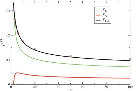
which agrees very well with simulations (Figure 7). Note thatP(UNr) approaches zero as slowly asO(1=log (n)).
Figure 6. Types of height-changing recombination events.The square indicates the new node created by re-grafting. It forms the new root in cases U, D and N. In case S, an existing internal node becomes the new root (empty square overlaid on noden1).
doi:10.1371/journal.pone.0060123.g006
Figure 7. Increase of tree height.ProbabilitiesP(r)UN(black),P(r)U (green) andP(r)N (red) of events that increase tree height as a function of sample sizen. Dots represent the values ofP(r)UNobtained by simulations using program ms [5] and selecting a random recombination event which is far from the sequence boundaries.
This result can also be derived directly by counting ARGs, since p(r)(T)corresponds to the distribution of a random tree in an ARG. We will consider the case of a recombination event at a given levelk and then average over all levels. To obtain the total number of ARGsAn,kwith a single recombination event at levelk, choose a tree at random (amongDLnDpossibilities), then choose the branch to be pruned (kpossibilities) and the branch to which it is re-grafted at the same or a higher level (Pk
j~1jpossibilities). Therefore,
An,k~
k2(kz1)
2 DLnD ð10Þ
The number of ARGs where the new tree is higher than the old one iskDLnD, because there is just one possibility of re-grafting, namely on the ancestral lineage above the root of the old tree. The probability of pruning at levelkin the old tree isPk~ktk=l. Therefore, one can average overp(r)(T)to obtainP(r)
UN~
Pn
k~2kEr(tk=l)kDLnD=An,k, which is identical to equation (9).
Focusing now on pruning of the root branches, we obtainPU analogously to equation (7). LetNk(nj)be the number of direct descendants of nodenjat levelk.Nk(nj)can take values0,1,2. The average value ofNk(nj)satisfies the recursion
N
Nkz1(nj)~NNk(nj) 1{ 1 k
N
Njz2(nj)~2
that has the solution
N Nk(nj)~
2(jz1) k{1 :
In particular, the average number of direct descendants of the root at level k is NNk(n0)~2=(k{1). The probability PU is a modification of equation (7): multiplying by the fraction of events that are actually of type U, i.e.Nk(n0)=k, one obtains
PU(T)~
Xn
k~2
ðtk
0
dt
l(T)Nk(n0)e {2ktk{P1
j~2e {2jtj
~1 l
Xn
k~2
Nk(n0)
1{e{2ktk
2k P
k{1
j~2e {2jtj:
ð11Þ
In contrast to equation (7), equation (11) cannot be easily simplified since it depends also on the topology. After averaging overp(r)(T), we obtain
P(Ur)~ 1 2an
12bnz 10
nz 2 nz1z
8 n2{19
ð12Þ
and
P(Nr)~1 an
10{6bn{ 6 n{
4 n2
, ð13Þ
wherebn~Pn {1 j~11=j2.
The probabilitiesP(Dr)andP (r)
S can be computed similarly to the above formulae, giving
PD(T)~
t2
l{
1{e{4t2 4l
z1 l
Xn
k~3
Nk(n0)
1{e{2ktk
2k P
k{1
j~3e
{2jtj1{e {4t2
2
ð14Þ
and
PS(T)~
1 l
Xn
k~3
Nk(n0)
P k{1
j~3 1{e{2ktk
2k P k{1
d~jz1e {2dtd j{1
j (1{e {2jtj)
zk{k1 tk{1{e {2ktk 2k 2 6 6 6 4 3 7 7 7 5
ð15Þ
(Text S1, Supporting Information eqs (4)–(9)). Alternatively, one may employ an argument based on symmetry properties of the ARG. Among two adjacent trees in the ARG, the left one is smaller or larger than the right one with equal probability. Therefore,
P(DSr)~P(UNr) : ð16Þ
The same is true when the root is only shifted. Thus,
P(Dr)~P(Ur): ð17Þ
Hence, by subtraction,
P(Sr)~P(Nr): ð18Þ
Note that the identities (17) and (18), being topological in nature, are also valid for models with variable population size. A related result about the probability that a random recombination event leaves tree height unchanged (1{P(UNr) {P(DSr)) has been obtained previously by Griffiths & Marjoram [24].
Equations (8), (11), (14), (15) are valid also when averaging over the distributionp(c)(T), instead of p(r)(T). However, exact results are available only for small sample sizes. For the case of arbitrary n we use the following Taylor approximation of the ratio moment
E X
l
^E(X) E(l) 1z
Var(l) E(l)2 z
Cov(X,l) E(X)E(l)
, ð19Þ
where E(X)=E(l) represents the desired probabilityP(c). When the expansion is truncated at zeroth order (i.e., replacing the first moment of the ratio by the ratio of first moments), one obtains the results analogous to equations (12), (13), (17) and (18). More detailed calculations are given in Text S1, Supporting Informa-tion eqs (10)–(12). These yield, for instance, the probability of increasing tree height
P(UNc) ^P(r)
UN 1z
bn a2 n
z 1 an
3=2{1=n{1=(nz1) n(nz1)=2{1
Note that the scaling factor on the right hand side in equation (20) approaches 1 very slowly with increasing n. The case P(UNc) is actually an exception since an exact formula exists [15] for all values of ; in fact,PUN(T) depends only onl(T), therefore it is sufficient to average this quantity over the distribution of l obtained in [15]. For small samples there is a considerable difference betweenP(UNc) andP
(r)
UN. For example, ifn~2, we have
P(UNc) ~0:55while onlyP(UNr) ~0:33.
Amount of change in height. The variation in heightDhhas a simple distribution. If the height increases, then the difference is given by the waiting time for coalescence of two lineages. It is
PU(DhDT)~2e
{2Dhg(Dh)P
U(T) ð21Þ
and
PN(DhDT)~2e{2Dhg(Dh)PN(T): ð22Þ
where g(x) is the Heaviside function, g(x)~1 if x§0 and 0 otherwise. If the height decreases because of an event of type D, its distribution is given by the waiting time for coalescence before timet2, equivalent to the ‘‘bounded coalescent’’ for two lineages [25]
PD(DhDT)~
2e{2(t2zDh)g({Dh)g(t 2zDh)
1{e{2t2 PD(T): ð23Þ
For events of type S, the variation in height is simply the waiting timet2of the tree
PS(DhDT)~d(Dhzt2)PS(T) , ð24Þ
where d(x) is the Dirac delta distribution. Averaging these quantities over p(r)(T) and using the symmetries of the ARG, we obtain
P(Ur)(Dh)~P(Dr)({Dh)~2e{2Dhg(Dh)P(r)
U ð25Þ and
P(Nr)(Dh)~P(Sr)({Dh)~2e{2Dhg(Dh)P(r)
N: ð26Þ i.e., all these variations in height are exponentially distributed for an average tree.
Taking expectations, the average change in height after one of these events is
DE(Dh)D~1=2 ,
irrespective of the type of event, i.e E(DhDU)~E(DhDN)~{E(DhDD)~{E(DhDS)~1=2. Comparing this to the average height of a tree,E(h)~1{1=n, one notices that a single recombination event changes tree height by 50% on average.
(c) Root Imbalance and Recombination
LetLn0 (Rn0) be the number of left (right) descendants of the root. We have Ln0zRn0~n. We call the random variable V~min (Ln0,Rn0) root imbalance. V is a coarse-grained measure of tree topology. A recombination event may or may not changeV
and a change ofVis neither sufficient nor necessary for a change in tree height. Since many recombination events induce rearrangements of the lower branches (close to the leafs) of the tree, they may affectVwithout affecting tree height. Still, large changes inVare often associated with height-changing recombi-nation events of type N or S and thus are associated with drastic changes of tree topology.
In this section we calculate the transition probabilitiesP(vDv0) forVunder a single recombination event, averaged over the initial tree. First, we focus on events of type UN, i.e. increasing height, and then we obtain the transition probabilities for all types of events separately.
Root imbalance and height-increasing events. Let thesize
of a branch be the number of leaves below the branch. A specific tree of sizencan be fully described by the probabilityPn,k(iDT) that a randomly chosen branch at levelk has size i. Averaging over trees of sizen, the probability that a branch of levelkhas size iis
Pn,k(i)~
n{i{1 k{2
= n{1 k{1
ð27Þ
[26]. LetPP~(UNr) (i)be the probability that the height increases and the pruned branch has sizei. It is obtained, similarly toP(UNr) , by multiplying each term of the sum in equation (7) by Pn,k(iDT). Thus, given a treeT,
~ P
PUN(iDT)~
Xn
k~2
ðtk
0
dt
l(T)Pn,k(iDT)e {2kt
P k{1
j~2e
{2jtj ð
28Þ
and, averaging overp(r)(T), one obtains
~ P
P(UNr) (i)~2 an
Xn
k~2
n{i{1 k{2
n{1 k{1
1
k(k{1)(kz1): ð29Þ
More generally, the probability that the pruned branch has sizei, given that recombination leads to an increase in height, is simply ~
P
P(r)(iDUN)~PP~(r) UN(i)=P
(r)
UN. The random variableVcan take values between 1 and n=2 and is the folded version of the random variableiwhich ranges from1ton{1. Hence, the distribution of V, after an event that increases tree height, is
P(UNr) (v)~
~ P
P(UNr) (v)zPP~(UNr) (n{v) (1zd2v,n)
and the distribution ofV, conditioned on tree height increase, is
P(r)(vDUN)~P
(r) UN(v)
P(UNr) , ð30Þ
as illustrated in Figure S3.
need information about the actual sizekat levelkof the subtree of sizev0of the root. We denote the distribution ofkbyP(kDv0,k,n) and the distribution ofigiven the sizeskandv0of its root subtree at levelskandnbyP(iDk,v0). Note thatidoes not depend onknor on
n, but only on the size of the root subtree to which it belongs (see Figure S4). Therefore we have
Pn,k(iDv0)~
X
min (v0,k{1)
k~i
P(iDk,v0)
k
kzP(iDk{k,n{v0) k{k
k
P(kDv0,k,n) ð31Þ
The probabilityP(iDk,v0)is equal to
P(iDk,v0)~Pv0,k(i)zdi,v0dk,1~
v0{i{1
k{2
v0{1
k{1
zdi,v0dk,1 ð32Þ
as can be shown by considering the corresponding subtree of the root as the whole tree and using equation (27). The probability P(kDv0,k,n) depends only on the topology, therefore it can be obtained by counting the number of labelled coalescent trees (http://arxiv.org/abs/1112.1295v2) with a root branch of sizev0 in the whole tree that reduces to sizekat levelk, denoted byLn,v0,k,k, and dividing by the total number of trees with a root branch of size
v0, denoted by Ln,v0. Using thatDLnD~n!(n{1)!=2n{1, that the coalescent process induces a uniform distribution onLnand that the distribution ofv0is2=(n{1)(1zd2v0,n)[27], we have
DLn,v0D~
2DLnD (n{1)(1zd2v0,n)
~ n!(n{2)! 2n{2(1zd
2v0,n)
ð33Þ
The set of all trees inLn,v0,k,kcan be generated in the following way: (i) choosev0leafs out ofn; (ii) choose an relative order of the
n{2coalescent events among the two subsets withv0andn{v0 leafs such that among the firstn{keventsv0{kevents belong to the first subset andn{v0{kzkbelong to the second; (iii) choose a topology for the root subtree of sizev0; (iv) choose a topology for the complementary subtree of the root. This process generates exactly once all trees in Ln,v0,k,k, except for the case v0~n=2, where each tree is generated twice. Therefore, we have
DLn,v0,k,kD
~ 1
1zd2v0,n n
v0
! n{k
v0{k
! k{2
k{1 !
DLv0DDLn{v0D: ð34Þ
Taking the ratio of tree counts, we obtain an hypergeometric distribution
P(kDv0,k,n)~
DLn,v0,k,kD DLn,v0D
~Hypv
0{1,k{2;n{2(k{1): ð35Þ
Finally, inserting the results (32) and (35) into (31), we obtain
Pn,k(iDv0)
~ di,v0
n{v0{1
k{2 !
zdi,n{v0
v0{1
k{2 !
kn{2
k{2
! z
n{i{2
k{3 !
kn{2
k{2 ! :
ð36Þ
2Bk{3,v0{i{1;n{i{2zMk{3,v0{i{1;n{i{2
z (k{1)Bk{3,v0{1;n{i{2{Mk{3,v0{1;n{i{2
2 6 4 3 7 5,
whereBx,y;zandMx,y;zare the normalization and the mean (i.e., the zeroth and first moment) of the hypergeometric distribution with parameters x, y and z, if they satisfy 0ƒx,yƒz, and 0
otherwise. Note thatMx,y;z~ xy
z Bx,y;z.
As before, we introducePn,k(iDv0)in equation (7) to obtain
~ P
P(UNr) (iDv0)~
2 an
Xn
k~2
Pn,k(iDv0)
1
k(k{1)(kz1) ð37Þ and, finally, the result
P(UNr) (vDv0)~ ~ P
P(UNr) (vDv0)zPP~(UNr) (n{vDv0)
(1zd2v,n)
ð38Þ
P(r)(vDUN,v 0)~
P(UNr) (vDv0)
P n{1
j~1 ~ P P(UNr) (jDv0)
ð39Þ
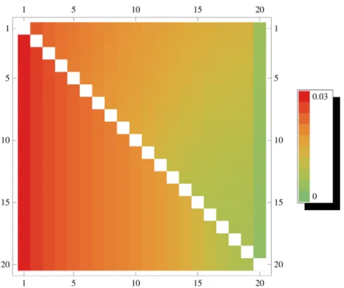
Figures 8 and S5 illustrate these probabilities. With a recombina-tion event of type N,vtends to change to smaller values. Thus, the tree becomes more unbalanced. However, by far the highest probability is attained forv~v0, irrespective ofv0 and mainly due to events of type U. This case is omitted from the figures for clarity.
Other recombination events that change root im-balance. Now we consider all possible recombination events that changeV. Events of type U and D do not changeV, so they can be ignored. Apart from the events of type N that we discussed above, other relevant recombination events are of type S and of type R (‘root remains’), i.e. any event which leaves the root untouched. To compute the probability of a change inVfor these types of events, we use the fact that random trees from an ARG have the distribution p(r)(T) and that the probability of each labelled ARG topology is the same. Due to this, we need only count the number of ARGs with a single recombination event at levelkcompatible with root imbalancesv0andv, and denoted by An,k,v0,v,S and An,k,v0,v,R. Then, we divide by the total number An,k,v0 of ARGs with a recombination at level k and root imbalancev0for the original tree. Putting everything together, we obtain
P(Rr)(vDv0)~
1 an
Xn
k~3
1 k2(kz1)
1 n{2 k{2
n{v0zv{2
k{3
H(v0{v{1)(2(k{1)Bk{3,v{1,n{v0zv{2z
z(k{3)Mk{3,v{1,n{v0zv{2{Qk{3,v{1,n{v0zv{2)z
z 1
(1zd2v,n)
n{vzv0{2
k{3 !
H(v{v0{1)(2(k{1)
Bk{3,v0{1,n{vzv0{2z
z(k{3)Mk{3,v0{1,n{vzv0{2{Qk{3,v0{1,n{vzv0{2)z
z 1
(1zd2v,n)
vzv0{2
k{3 !
H(n{v0{v{1)(2(k{1)
Bk{3,v0{1,vzv0{2z
z(k{3)Mk{3,v0{1,vzv0{2{Qk{3,v0{1,vzv0{2)
i ,
where Qx,y;z is the second moment of the hypergeometric distribution with parameters x, y and z satisfying 0ƒx,yƒz, and0otherwise, andH(n)is the Heaviside function,H(n)~1if n§0and 0 otherwise. Note that the ARG symmetries imply the non-trivial relation
P(Rr)(vDv0)~P(Rr)(v0Dv)
1zd2v0,n 1zd2v,n
: ð41Þ
The relative importance ofP(Rr) versusPUN(r) andP(DSr) is shown in Figure S6.
The contribution for events of type S can be obtained using the symmetry properties of the ARG. In fact, an ARG with a recombination event of type S changingv0tovis equivalent to an ARG with an event of type N changingvtov0. Therefore,
P(DSr)(vDv0)~P(UNr) (v0Dv)
1zd2v0,n 1zd2v,n
: ð42Þ
This result is essentially the transpose of the one shown in Figure 8, i.e. after an event of Type S,vhas an almost uniform distribution irrespective ofv0.
Finally, the transition probability is
P(r)(vDv 0)
~
v=v0: P(UNr) (vDv0)zPDS(r)(vDv0)zPR(r)(vDv0)
v~v0: 1{ P
v=v0
P(UNr) (vDv0)zP(DSr)(vDv0)zPR(r)(vDv0)
0
B @
ð43Þ
This distribution is shown in Figures S7 and S8 forn~40.
Figure 8. Transition probabilities ofV.DistributionP(r)(vDUN,v
0)as a function ofv(horizontal axis) andv0(vertical axis) forn~40. The diagonal terms (v~v0) are not shown.
(d) Hidden and Silent Recombination Events
Counting ARGs we now determine the fraction of hidden
recombination events, i.e. those which neither change tree topology nor branch lengths. Since these events are ‘invisible’ when analysing sequence polymorphisms or haplotype structure, their frequency can only be estimated by theoretical means.
Hidden recombination events are caused by pruning and re-grafting on the same branch (see Figure 2D). LetAn,k,Hdenote the number of ARGs with a hidden event at level k. Since ARG topologies are equiprobable underp(r)(T), the probability that a recombination event is hidden is
P(Hr)~X
n
k~2
Pk An,k,H
An,k
, ð44Þ
wherePk~E(ktk=l)~((k{1)an){1is the probability of pruning at levelk. To calculateAn,k,H we need to consider the following ingredients. A branch pruned under nodenjcan be regrafted in k{j{1topologically inequivalent ways on the same branch (but possibly on different levels). This number has to be multiplied by the number of branches under node nj at level k (denoted by Nk(nj)). Then, one has to sum over all possible nodesnjand over all possible initial treesT[Ln. This yields
An,k,H~ X
T[Ln X k{2
j~0
Nk(nj)(k{j{1)
~X
k{2
j~0 N
Nk(nj)(k{j{1)DLnD
ð45Þ
Combining eqs (44) and (45) we obtain
P(Hr)~ Xn
k~2
1 (k{1)an
Pk{2
j~0NNk(nj)(k{j{1)DLnD k2(kz1)DLnD=2
~ 2 3an
1{1 n
:
ð46Þ
This means that the fraction of hidden recombination events is of the order O(1=log (n)). They are quite frequent for small to moderaten, but become increasingly rare with increasingn. Still, even when n~1000, about 9% of all recombination events are hidden.
Using the same technique of counting ARGs also the fraction of silent recombination events (i.e. events that do not change topology but that may change branch lengths) can be obtained. We start by counting events that are silent but not hidden. Given a tree, select a branch for pruning. Then, there are exactly two ways for re-grafting: either on the branch immediately above or on the branch immediately below the old parent node of the pruned branch (Figure 2B or C), but not on the pruned branch itself (the latter would be a hidden event). Performing similar calculations as before we obtain
P(silentr) {P(Hr)~ Xn
k~2
1 (k{1)an
An,k,sil{H{ An,k
~X
n
k~2
1 (k{1)an
Pk{2
j~02NNk(nj)DLnD k2(kz1)DL
nD=2
~1 an
1{ 2
n(nz1)
:
ð47Þ
Therefore,
P(silentr) ~ 1 3an
5{8 nz
6 nz1
: ð48Þ
Note that the following holds:
P(silentr) ~PUNDS(r) zP(Hr): ð49Þ
An intuitive explanation is the following: for any pruning point, there are two possible ways for re-grafting such that tree topology remains unchanged and there is exactly one way for re-grafting which leads to an increase of tree height. Therefore, Psilent(r) {PH(r)~2P(UNr) . Then, eq (49) follows from symmetry of the ARG. Note that this argument is topological and does not depend on waiting times, i.e. branch lengths.
(e) Correlation Lengths
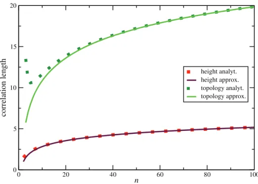
Since the spatial coalescent is a non-Markovian process, it is important to know over which chromosomal distances correlation and statistical dependence among trees persist. Correlation between trees, measured by any well-behaved tree statistic, decreases with distance. An interesting question is how quickly recombination reduces correlation. The answer depends on the particular statistic which is employed to measure correlation. Topology based statistics, such asV(measuring imbalance at the root) or Colless’ index [28] (measuring imbalance at all internal nodes), behave differently from length based statistics, such as tree height (Figure 9).
We use our above results regarding events of type U, D, N, S and R to give a quantitative answer. The idea is to approximate the correlation length for a statistic by the inverse of the probability of recombination events that have a strong impact on this statistic.
Events of type U or D change height, but leave the topology unchanged. Events of type R preserve height but alter topology. Events of type N or S may change both, height and topology. They also lead to the fastest decay of correlation.
L(topr) 1 P(NSr)
an
2(10{p2)&3:83an: ð50Þ
It Increases Logarithmically inn(Figure 9)
To translate this into physical length, we assume that the distance between two consecutive recombination events is exponentially distributed with mean 1=(rl(T)). Averaging over p(r)(T) we obtain1=(ra
n). Therefore, distanceltopbetween two events of type N or S is approximately
ltop~ L(topr)
ran
* 1
2(10{p2)r*
3:83
r , ð51Þ
independent ofn. For example, if the scaled recombination rate is
r&10{3, the genomic distance between such events is about4kb. Assuming that also the scaled mutation rate ish&10{3per bp and assuming n~100, an interval between drastic recombination events of type N or S contains about4a99&20polymorphic sites. This number should be sufficiently high to enable at least a rough tree re-construction from SNP data, and to estimate V. It will probably not be sufficient for the reconstruction of the fine topological structure of the lower branches.
To estimate the correlation length ofV, also events of type R need to be taken into account. In fact, changes inVoccur more often than events of type N or S. Using equation (43), we determined the run-length ofV, i.e. the number of recombination events that occur before a change inVhappens. Considering a random initial tree, an estimate for the run-length is given by
LV~ 1
1{P(r)(vDv): ð52Þ
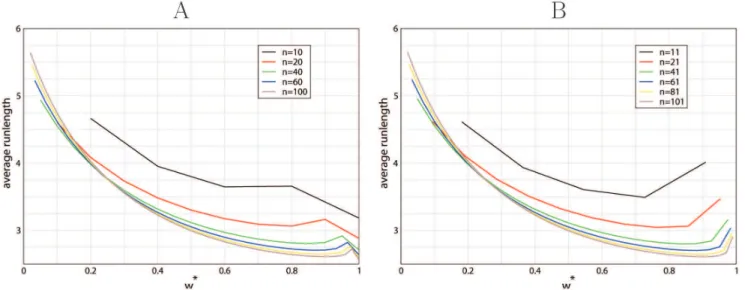
The run-length is longer for more imbalanced trees, but always on the order of a few recombination events (between 2 and 6; Figure 10). This is also a reasonable estimate for the correlation length of the fine topological structure.
We now consider correlation in tree height. Height can change by events U,D,N and S. The average change in height is the same, DDhD~1=2, for all these events. Therefore, correlation length can be estimated as
L(hr)*1=P (r) UNDS:
Since
P(UNDSr) ~2P(UNr) is between0:25and0:3for 20=n=100 (Figure 7), drastic changes in height are expected on average every3to 4 recombination events. More generally, the correlation length also increases logarithmically innand is
L(hr)*an: ð53Þ
For the physical correlation length we have.
lh~L (r) h
ran *1
r: ð54Þ
This is only about a quarter of the topological correlation length. Therefore, an exact reconstruction of tree height is difficult. For instance, forn~100andh~r~10{3, one would have on average only5SNPs to estimate height or other tree parameters.
For the case n~2, Hudson [21] gives a formula for the correlation between the heights of two trees in dependence of the recombination rate r. The formula predicts that the correlation drops to about 0:5 with r1:4, i.e. after approximately 1.4
Figure 9. Correlation lengthL(r)
recombination events. Our rough estimate for the correlation length in this case is1=P(UNDSr) ~1:5, and in good agreement with Hudson’s result.
Finally, we briefly comment that linkage disequilibrium and haplotype block size depend strongly on the number and distribution of mutation and recombination events along coales-cent trees, i.e. they depend strongly on tree topology and length. Since topology can in practice only be indirectly estimated from polymorphism patterns, not all changes in topology are actually visible for these statistics. The correlation lengths estimated from experimental data will tend to be larger than the theoretical estimates presented here. Assuming that haplotype blocks are mostly delimited by ‘drastic’ recombination events, involving a change of topology, we estimate the size of these haplotype fragmentsLh, centered at some positionxwith a treeT. Assuming further that neither tree length l(T) nor the probability of topology-changing drastic recombination events Ptd(T) change much after a ‘non-drastic’ recombination event, the probability distribution for the haplotype sizes is
P(LhDT)~e{rl(T)Ptd(T)Lhrl(T)P
td(T): ð55Þ
The average size is then
E(LhDT)~1=(rl(T)Ptd(T)): ð56Þ
The class of drastic recombination events that should be considered to determinePtd(T) is probably larger than the class of type N and S events. However,Ptd(T)~PNS(T)is a reasonable lower bound approximation.
Discussion
We have considered the effect of single recombination events on coalescent tree topology and explicitly determined the probability with which recombination triggers ‘drastic’ changes. We consider a change to be drastic if it leads to a change of tree height or of tree
imbalance. These types of events are of practical interest because both have an effect on the pattern of polymorphic sites which are informative for genealogical reconstruction and evolutionary inferences. The primary effect of height change is upon the number of mutations, while a change in tree imbalance primarily affects the mutation site frequency spectrum.
Our results show important qualitative differences for the two types. The average change in height is quite drastic per se (50% of average tree height), while the average change in imbalance is quite mild, with large jumps occuring only very rarely. Our results hold for the standard neutral model, i.e. a model with constant population size and without substructure. As such, our results may serve as the analytical reference case for constructing formal tests of the neutral evolution hypothesis. For instance, the probabilities of height or topology change are markedly altered in the presence of selective sweeps, i.e. the fast fixation of a mutant allele due to positive selection. Recombination close to the sweep site, where tree height is severely reduced [29], tends to lead to both a drastic increase of tree height and highly imbalanced trees [16,18]. In contrast, variable population size leaves a different signature on the probabilities of drastic recombination events. Non-constancy ofNis reflected in branch length variation, but it has no impact on the branching pattern, i.e. on topology. In fact, if panmixis continues to hold, the probability distribution of tree topologies does not depend on population size. Variation ofN affects only branch lengths and waiting times. Since all our results, averaged overp(r)(T), depend implicitly on the first moments of the waiting times through the quantityPk~kE(tk=l), they can in principle be adapted to models with variable population size using the theory developed earlier [26,30]. A detailed treatment is left to further investigation. Here we just note that the relations (17), (18) and (49) are valid for all models of variable population size.
Population substructure is another important case of deviation from the standard neutral model. Restricted gene flow between sub-populations strongly affects the transition probabilities of root imbalance, but less the distribution of height change. A more detailed discussion of the impact of these evolutionary scenarios upon a test statistic of the neutral evolution hypothesis is given in [18].
Figure 10. Run length1=(1{P(r)(vDv))as a function ofv~2v
n for even sample sizes (A) (n~10,20,40,60,80,100) and for odd sample
sizes (B) (n~11,21,41,61,81,101).
We have derived a number of further results which shed more light on the details and consequences of recombination. We analysed the correlation length between trees on a recombining chromosome and showed that topological correlation is generally longer-ranging than correlation in tree height. Still, for both types very few recombination events – on the order of ten – are sufficient to unlink the genealogical histories of two genomic fragments, given standard neutral conditions. The calculations also make clear that correlation length (number of recombinations) scales logarithmically in n. This is important to take into account for deep sequencing association studies.
It is perhaps surprising to see that a considerable fraction of recombination events remains hidden. Even for large sample sizes, about10%of the recombination events are not visible. An even larger fraction is silent, i.e. does not cause topological changes of the underlying genealogy.
Analyzing root imbalance in more detail, we found that the distribution ofV-run lengths is biased towards unbalanced trees: under the standard neutral model, unbalanced trees tend to span larger genomic regions than balanced trees. Interestingly, theV -run length, when normalized, is asymptotically independent ofn. Our results provide a basis to tackle problems of correlation between tree statistics in coalescent models. They extend known results, such as the one by Hudson [21] concerning tree height correlation, to the more general case of arbitrary sample sizen.
Some of the quantities studied here involve counting problems of ancestral recombination graphs with a single recombination event. These problems are related to counting problems of phylogenetic networks [31]. Unlike counting problems of trees, which can often be tackled by generating function techniques ([20], arxiv.org/abs/1112.1295v2, arxiv.org/abs/1202.5668v3), only few results are available for tree-like structures with independent cycles so far [32]. Our results represent a step towards a combinatorial treatment of these problems.
Supporting Information
Figure S1 Probability of increasing height after a
recom-bination event as a function of the total tree lengthl.
(PDF)
Figure S2 Probability of recombination events P(NSr)
which change tree height and topology as a function of
the sample sizen.
(PDF)
Figure S3 Distribution P(r)(vDUN) of V after an event
that increases tree height, forn~20.
(PDF)
Figure S4 Illustration of the sizesxandyof the subtrees
at the levels k and j corresponding to pruning and
regrafting, respectively.
(PDF)
Figure S5 Probability distribution P(r)(vDUN,v 0) for
v0~1,5,10,15 (in blue, pink, yellow, green) and n~40.
For clarity, only the probabilities forv=v0are shown.
(PDF)
Figure S6 RatioP(UNDSr) (vDv0)=P(Rr)(vDv0)as a function ofv
(x-axis) and v0 (y-axis) for n~40. For clarity, only the
probabilities forv=v0are shown. (PDF)
Figure S7 Distribution P(r)(vDv
0) of V forv0~1,5,10,15
(in blue, pink, yellow, green) andn~40.
(PDF)
Figure S8 DistributionP(r)(vDv
0) as a function of v (x
-axis) and v0 (y-axis) for n~40. For clarity, only the
probabilities forv=v0are shown.
(PDF)
Text S1 Supporting information.
(PDF)
Acknowledgments
We would like to thank Jeff Thorne and two anonymous reviewers for very constructive comments, and A. Klassmann and S. Ramos-Onsins for numerous discussions.
Author Contributions
Analyzed the data: LF TW. Wrote the paper: LF TW. Designed the study: TW LF. Performed calculations and derived theorems: LF FD. Performed computer simulations: LF TW.
References
1. Kingman JFC (1982) The coalescent. Stochastic Processes and their Applications 13: 235–248.
2. Hudson RR (1990) Gene genealogies and the coalescent process. In: Oxford Surveys in Evolutionary Biology, Oxford University Press, volume 7. 1–44. 3. Wakeley J (2009) Coalescent theory – an introduction. Greenwood Village,
Colorado: Roberts&Company.
4. Kimura M (1987) Molecular evolutionary clock and the neutral theory. J Mol Evol 26: 24–33.
5. Hudson RR (2002) Generating samples under a Wright-Fisher neutral model of genetic variation. Bioinformatics 18: 337–338.
6. Kim Y, Wiehe T (2009) Simulation of DNA sequence evolution under models of recent directional selection. Brief Bioinform 10: 84–96.
7. Ewing G, Hermisson J (2010) MSMS: a coalescent simulation program including recombination, demographic structure and selection at a single locus. Bioinformatics 26: 2064–2065.
8. Griffiths RC (1984) Asymptotic line-of-descent distributions. J Math Biol 21: 67– 75.
9. Sagitov S (1999) The general coalescent with asynchronous mergers of ancestral lines. J Appl Probab 36: 1116–1125.
10. Greven A, Pfaffelhuber P, Winter A (2009) Convergence in distribution of random metric measure spaces (L-coalescent measure trees). Probab Theory Relat Fields 145: 285–322.
11. Bhaskar A, Kamm JA, Song YS (2012) Approximate sampling formulae for general finite-alleles models of mutation. Adv Appl Probab 44: 408–428. 12. Angel O, Berestycki N, Limic V (2012) Global divergence of spatial coalescents.
Probab Theory Relat Fields 152: 625–679.
13. Griffiths RC, Marjoram P (1996) Ancestral inference from samples of DNA sequences with recombination. J Comput Biol 3: 479–502.
14. Li H, Durbin R (2011) Inference of human population history from individual whole-genome sequences. Nature 475: 493–496.
15. Wiuf C, Hein J (1999) Recombination as a point process along sequences. Theor Popul Biol 55: 248–259.
16. Fay J, Wu C (2000) Hitchhiking under positive Darwinian selection. Genetics 155: 1405–1413.
17. Li H (2011) A new test for detecting recent positive selection that is free from the confounding impacts of demography. Mol Biol Evol 28: 365–375.
18. Li H, Wiehe T (2012) Coalescent tree imbalance as an indicator of selective sweeps. (in review).
19. Murtagh F (1984) Counting dendrograms: A survey. Discrete Applied Mathematics 7: 191–199.
20. Disanto F, Wiehe T (2013) Exact enumeration of cherries and pitchforks in ranked trees under the coalescent model. Mathematical Biosciences 242: 195– 200.
21. Hudson R (1983) Properties of a neutral allele model with intragenic recombination. Theor Popul Biol 23: 183–201.
22. Wiuf C (2006) Consistency of estimators of population scaled parameters using composite likelihood. J Math Biol 53: 821–841.
24. Griffiths RC, Marjoram P (1997) An ancestral recombination graph. In: Progress in population genetics and human evolution (Minneapolis, MN, 1994), New York: Springer, volume 87 of IMA Vol. Math. Appl. 257–270. 25. Rasmussen M, Kellis M (2012) Unified modeling of gene duplication, loss, and
coalescence using a locus tree. Genome Res 22: 755–765.
26. Zivkovic D, Wiehe T (2008) Second-order moments of segregating sites under variable population size. Genetics 180: 341–357.
27. Tajima F (1983) Evolutionary relationship of DNA sequences in finite populations. Genetics 105: 437–460.
28. Colless DH (1982) Review: [untitled]. Systematic Zoology 31: 100–104.
29. Kaplan N, Hudson R, Langley C (1989) The ‘‘hitchhiking effect’’ revisited. Genetics 123: 887–899.
30. Griffiths RC, Tavare´ S (2003) The genealogy of a neutral mutation. In: Green P, Hjort N, Richardson S, editors, Highly Structured Stochastic Systems, Oxford Statistical Science Series, Oxford University Press, volume 27. 393–412. 31. Huson DH, Rupp R, Scornavacca C (2011) Phylogenetic Networks: Concepts,
Algorithms and Applications. Cambridge University Press.
![Figure 5. Height of neutral coalescent trees along the genome. One simulation run using ms [5] with n~20 and r~4Nr~10 { 3](https://thumb-eu.123doks.com/thumbv2/123dok_br/18291069.346620/5.918.88.810.85.291/figure-height-neutral-coalescent-trees-genome-simulation-using.webp)