Braz. J. Chem. Eng. vol.31 número4

(1)

ISSN 0104-6632 Printed in Brazil

www.abeq.org.br/bjche

Vol. 31, No. 04, pp. 967 - 975, October - December, 2014 dx.doi.org/10.1590/0104-6632.20140314s00002692

Brazilian Journal

of Chemical

Engineering

A MODIFIED ORTHOGONAL COLLOCATION

METHOD FOR REACTION DIFFUSION

PROBLEMS

M. Soliman

1,2

, Y. Al-Zeghayer

1

and A. Ajbar

3* 1

Department of Chemical Engineering, College of Engineering, King Saudi University, P.O. Box 800, Riyadh, 11421, Saudi Arabia.

E-mail: yszs@ksu.edu.sa

2

Department of Chemical Engineering, The British University in Egypt, El-Shorouk City, Egypt. E-mail: moustafa.Aly@bue.edu.org

3

Department of Chemical Engineering, King Saud University, P.O. Box 800 Riyadh 11421, Saudi Arabia. Phone: ++ 966-1-4676843, Fax: ++ 966-1478770

E-mail: aajbar@ksu.edu.sa

(Submitted: July 5, 2013 ; Revised: January 27, 2014 ; Accepted: February 1, 2014)

Abstract - A low-order collocation method is often useful in revealing the main features such as

concentration and temperature profiles and the effectiveness factor for porous catalyst particles. Two modifications are introduced in this paper to make the method more efficient. The first modification is to add an extra collocation point at the center of the particle. It is shown that such extra point introduces a single variable non-linear equation to be solved after obtaining the standard collocation method solution. In the second modification, the polynomial solution obtained from the application of the orthogonal collocation method is transformed to a rational function form. These two modifications are applied to specific examples and it is shown that they can improve the performance of collocation methods in general and the one-point collocation method in particular.

Keywords: Orthogonal collocation; Jacobi polynomials; Interpolation; Reaction diffusion; Catalyst particle.

INTRODUCTION

In the method of weighted residuals, we seek a solution for a differential equation in terms of a polynomial with unknown coefficients to be deter-mined such that certain criteria are satisfied. These criteria are usually chosen such that the integrals of the weighted residual, which is obtained by substi-tuting the assumed solution in the differential equa-tion written with one of its sides as zero, are zeros. Depending on the weight, we obtain methods like the Galerkin method, least square methods, the method of moments, and collocation methods. In collocation methods, we would like to have the residual to be zeros at particular points called collocation points. If the collocation points are the zeros of orthogonal

polynomials, the method is called orthogonal collo-cation. In all methods of weighted residuals, a non-linear ordinary differential equation is approximated by a set of non-linear algebraic equations.

The orthogonal collocation method was developed by Villadsen and Stewart (1967). It was then subse-quently studied and applied to many chemical engi-neering problems by several authors (Finalyson, 1972; Villadsen and Michelsen, 1978; Finalyson, 1980; Torres et al., 2000; Biscaia Junior et al., 2001).

(2)

determined, we use a different approach in this pa-per. Having obtained a polynomial solution, we con-vert this solution into a rational function.

Solution of catalytic reactor models requires the solution of a set of differential equations represent-ing the phenomena of diffusion with chemical reac-tion inside the pores of the catalyst particles at each location along the reactor. It is clear that such calcu-lations would require excessive computation time. It is our objective in this paper to make the method of orthogonal collocation more efficient in order to reduce the computational load.

In the next sections we introduce Jacobi polyno-mials, and then we introduce the standard method of orthogonal collocation. This is followed by present-ing the modifications. Then we derive formulae for the effectiveness factor calculation. Finally we apply the method to some problems of diffusion and reac-tion in catalyst particles.

JACOBI POLYNOMIALS

Usually orthogonal polynomials are defined on the closed interval [-1, 1]. However by simple linear transformation, we can change the definition to any other closed interval. For the purpose of this study we would like to define the polynomials in the inter-val [0, 1]. In this case they are called "shifted" poly-nomials. However, we will drop the word "shifted" for brevity.

The Jacobi polynomials P_n( , )α β of degree n are de-fined such that they satisfy the orthogonality con-ditions (Villadsen and Stewart, 1967)

1

( , ) ( , ) 0

( ) _n ( ) _m ( ) 0 ( )

w x P α β x Pα β x dx= n≠m

∫

(1)

and

1

( , ) ( , ) 0

( ) _n ( ) _m ( ) _n 0 ( )

w x P α β x Pα β x dx=C > n=m

∫

(2)

where w(x) is the weighting function for the or-thogonality conditions and _Cn is a constant. For Jacobi polynomials,

( ) (1 ) , , 1

w x = −x α βx α β > − (3)

Thus α, β are the indices of the weight function

w(x). We will drop the superscripts α, β for brevity.

Jacobi polynomials satisfy the differential equation:

2 2

( ) ( )

(1 ) [(1 ) ( 2) ]

( 1) ( )

n n

n

d P x dP x

x x x

dx dx

n n P x

− + + β − α + β + =

− + α + β + (4)

For the case of α = 1 which is of interest in this work, this equation can be written as,

2 2

[(1 ) ( )] [(1 ) ( )]

( 1)

[ ( 2) (1 )] ( )

n n

n

d x P x d x P x x

dx dx

n n P x

− _{+ β +} − ₌

− + β + − + β (5)

The first member of the Jacobi polynomials, P0,is of course a constant; thus from Equation (1) for α= 1, we have:

1

0

(1 ) _n( ) 0 ( 0)

xβ −x P x dx= n>

∫

(6)

MATHEMATICAL FORMULATION AND SOLUTION BY THE STANDARD

COLLOCATION METHOD

Mathematical Formulation

Consider a reaction with a dimensionless rate R(u), where u is the dimensionless concentration. The reaction takes place isothermally inside a catalyst particle with no external resistance to mass transfer. We may write the describing equation as:

2

1

[ s ] ( )

s

d du

r R u dr dr

r = φ (7)

with the boundary conditions:

(1) 1

u = (8)

0 0 r

du

dr = = (9)

(3)

A Modified Orthogonal Collocation Method for Reaction Diffusion Problems 969

rate R(u) is normalized with respect to the reaction rate at the external surface of the catalyst and, hence, at the external surface r=1, u = 1 and R (1)= 1. The effectiveness factor ηis given by:

2

(s 1)du dr

+ η =

φ r=1=

1

0

(s+1)

∫

r R u drs ( ) (10)

Since the boundary condition (9) implies that the solution will be symmetric with respect to (r), we introduce the transformation:

2

x=r (11)

so that the problem is changed to:

2

2 2

4xd u 2(s 1)du R u( )

dx

dx + + = φ (12)

and

(1) 1

u = (13)

The effectiveness factor is given by:

1

0

(s 1) r R u drs ( )

η = +

∫

1 ( 1) 2 0

( 1)

( ) 2

s

x R u dx

− +

=

∫

(14)

Except for a few cases, such as isothermal first-order and zero-first-order reactions, the analytical solu-tion of the boundary value problem, Eqs. (7)-(9) or Eqs. (12), (13) is, in general, not feasible, and the problem can only be solved numerically. In the case when the effectiveness factor is calculated repeat-edly, such as in the simulation of packed bed cata-lytic reactors, we need a fast and efficient numerical method. A simple, convenient and easy approach to solve such problems is through the use of the or-thogonal collocation method.It is the purpose of this paper to introduce two modifications to the colloca-tion method which may yield somewhat higher accu-racy for the concentration profile and the effective-ness factor than the standard collocation method.

Collocation Solution Representation

In the orthogonal collocation method, we repre-sent the solution as a polynomial with unknown co-efficients to be determined such that the differential equation is satisfied at certain points. A better way of

writing a polynomial approximation of a function in terms of its values (ordinates) at certain points is through the Lagrange interpolation formula. It has many advantages compared to the straightforward polynomial. First the solution is obtained directly at collocation points. Secondly, when we have a non-linear differential equation, we could have a very good initial guess for the ordinates _ui's which lie between 0 and 1, whereas we do not know the range of the parameters in the straightforward polynomial. Thirdly and most important, we can easily derive formulae for the derivatives using the Lagrange in-terpolation formula. Fourthly, the same Lagrange formula can then be used to obtain the value of u at any point x

∈ [0, 1].

The Lagrange interpolation formula is given by:

1

( ) ( ) ( ) ( )

N

i i i

i

u x u x l x u x

+

=

= =

∑

(15)

where

1 1,

( ) ( )

N

j i

j j i _i _j

x x l x

x x

+

= ≠

− = Π

− (16)

are the Lagrange polynomials.

From Equation (15), the first and second order derivatives of any function u(x) expressed in terms of Lagrange polynomials and at a collocation point _{x = xi} can be written as:

1

i

N

x x ij j

j

du

a u dx

+ =

=

∑

(17)

1 2

2

1

i

N

x x ij j

j

d u

b u dx

+ =

=

∑

(18)

where

(1)

( )

ij j i

a =l x (19)

(2)

( )

ij j i

b =l x (20)

An efficient method for calculating the elements

aij and bij is given in the book of Villadsen and

Michelsen (1978).

(4)

1 1 1 2

1 0

( 1)

( ( )) ( )

2

s i N

i i

i

s

x R u x dx w R u

− = +

− +

η =

∫

=

∑

(21)

The weights of the quadrature are obtained by the procedure described by Villadsen and Michelsen (1978). This formula uses one extra point in x=1, and the zeros of the Lagrange polynomial are calculated using (α+1) instead of only α (Villadsen and Michelsen, 1978).

The collocation points are the zeros of the Jacobi polynomials suitable for the geometry of the catalyst particle. In our case, we use the Jacobi polynomials indices α= 1, β= (s-1)/2

Application of One-Point Standard Collocation to a First-Order Reaction

For a first-order polynomial with the function value given as u(1) at x = 1 and u (x₁) at x = x₁, the Lagrange interpolation formula is given by:

1

1 1

( ) ( 1)

( ) (1) ( )

(1 ) ( 1)

x x x

u x u u x x x

− −

= +

− − (22)

This formula satisfies the values of u at x = 1, and at x = x₁_.

Now if we choose x₁ to be the zero of a Jacobi orthogonal polynomial P1(x) such that α = 1, β = (s-1)/2, we obtain:

1

1 5

s x

s

+ =

+ (23)

For a first-order reaction, Equation (12) becomes:

1

2 2

2

1 1

4 2( 1)

( 1)( 5)

(1 ( )) ( )

2

x x

d u du x s

dx dx

s s

u x u x

=

⎡ ⎤

+ +

⎢ ⎥

⎣ ⎦

+ +

= − = φ

(24)

and u(x) becomes:

2 2

(1 ) ( ) 1

2( 1)[1 2 / ( 1)( 5)]

x u x

s s s

φ −

= −

+ + φ + + (25)

One can show that this solution is accurate up to terms containing φ4 at x = x₁ and up to φ2 elsewhere. In addition, the effectiveness factor, given by the fol-lowing Equation (26), is accurate up to φ4.

1 1 ( 1)

2

0 0

1 ( 1) 1 2

1

1 1

0

1

2

( 1) ( 1)

2

( 1) ( ) ( 1)

[ (1) ( )]

2 (1 ) ( 1)

( 1) ( 5)

[ (1) ( )]

2( 3) 2( 3)

(1 )

( 3)( 5)

2

(1 )

( 1)( 5)

s s

s

s r udr x udx

s x x x

x u u x dx x x

s s

u u x

s s

−

+

η = + =

+ − −

= +

− −

+ +

= +

+ +

φ +

+ +

=

φ +

+ +

∫

(26)

MODIFIED COLLOCATION METHOD

Two modifications to the standard collocation method are now suggested to improve its perform-ance.

First Modification

One can show that, if we collocate the equations at an extra point in addition to those obtained as the zeros of the proper orthogonal polynomial, we will have the ordinate of this extra point appearing only in the collocation equation of this point. This ordi-nate will not appear or affect the other equations.

Let us add an extra collocation x0 point, prefera-bly at x = 0, and define ue such that

1 ₁ 1

0,

0 0

( ) ( ) ( ) ( ) ( )

N _N N

j

e i i i

j j i _i _j

i i

x x

u x u x l x u x x x

+ ₊ +

= ≠

= =

⎡ − ⎤

= ⎢ Π ₋ ⎥ =

⎢ ⎥

⎣ ⎦

∑

(27)

We notice that the term multiplying u x( ₀) is given by:

0

1

0 0

( 1)

( ) ( )

( 1)

N j

j _j

x x x

u x

x = x x

− −

= Π

− − (28)

(5)

un-A Modified Orthogonal Collocation Method for Reaction Diffusion Problems 971

known variable u x( ₀)which can be solved after solving the standard collocation equations. This extra point will also not affect the effectiveness factor.

Application of One Point Collocation First Modi-fication (mod 1) to a First-Order Reaction

Let us write the Lagrange interpolation formula in terms of ordinates at one interior collocation point x₁

besides at the boundary x = 1. We have:

1 1

( 1)

( ) (1) [ ( ) (1)]

( 1)

x

u x u u x u x

−

= + −

− (29)

Let us define another solution ue such that its

Lagrange interpolation formula in terms of ordinates at an interior collocation point x₁, besides at the boundary x = 1 and any point x0, is:

1 0

0 1

1 1 0

1 0

0 0 1

( )( )

( ) (1)

(1 )(1 )

( 1)( )

( )

( 1)( )

( )

( 1)( )

e

x x x x

u x u

x x x x x

u x x x x

x x x u x x x x

− − = − − − − + − − − − + − − (30)

Now if x = x1, we note that u xe( )1 = u x( )1 and

both 4

2 2

d u

dx + 2(s+1) du dx

at x = x₁ and the integral

1 ( 1) 2 0

( )

s

x u x dx

−

∫

do not

con-tain a term of ue (x₀). This means that, whatever the

value of ue (x₀), u(x₁) and the effectiveness factor η

will not change. This is the major strength of the collocation method as applied to the catalyst particle problem. The choice of x0, and thus ue(x₀), will only

affect the profile of ue (x). Now for an arbitrary x₀,

we could write from Equation (12):

0 2 2 2 0 1 0 2 0

4 2( 1)

4( 3) ( 5)

[1 ( )] [1 ( )]

(1 ) 2

( )

e e

x x

e

d u du x s

dx dx

s s

u x u x x u x = ⎡ ⎤ + + ⎢ ⎥ ⎣ ⎦ + + = − − − − = φ (31)

Thus, after calculating u(x₁) from Equation (25), we calculate ue(x₀) from Equation (31) to obtain:

2 1 0 0 2 0

4( 3) ( 5)

(1 ( ))

(1 ) 2

( ) 4( 3) (1 ) e s s u x x u x s x ⎡ + ₋ + ₋ ⎤ ⎢ ₋ ⎥ ⎣ ⎦ =

⎡ + _{+ φ} ⎤

⎢ ₋ ⎥ ⎣ ⎦ (32) and 2 2 4 1 2 2 0 (1 ) ( ) (1)

2

2( 1)(1 )

( 5)( 1)

(1 )( )

2 (1 )

8( 1)( 3)[1 ][1 ]

( 5)( 1) 4( 3)

e

x u x u

s

s s x x x

x s s

s s s

φ −

= −

φ

+ +

φ − −

+

φ − φ

+ + + +

+ + +

(33)

Now x0 can be chosen to improve the accuracy at a certain point. x0 can be chosen as zero so that we obtain a higher accuracy for the value of (u) at the center of the catalyst particle. In Soliman (1988) the choice x₀=x₁2 was made.

In summary, the modified one point collocation requires the solution of two algebraic equations sequentially and it makes the whole profile exact for terms up to φ4, whereas in the original one point collocation the solution is exact for terms up to φ4 only at the collocation point and up to φ2 elsewhere.

Second Modification

Let us form a rational functionu x_r( ) from the polynomial solution ( )u x , and u x_e( ) such that:

( ) ( )

( )

1 ( )

N r

N

u x CP x u x

CP x

+ =

+ (34)

where 1 ( ) ( ) N N i j

P x x x

=

= Π − (35)

and C is a constant to be estimated such that:

(0) (0) (0) (0) 1 (0) N r e N u CP u u CP + = =

(6)

Thus

(0)(1 (0))

( (0)) / (0)

1 (0)

e

N e

u u

C u P

u

−

= −

− (37)

This choice makes ur(x) equal to ue(x) at x = x1 and

x = x0.

Application of One Point Collocation Second Modi-fication (mod 2) to a First-Order Reaction

Now we apply the rational function approxima-tion to the diffusion reacapproxima-tion problem with first order reaction rate, where:

( )

R u =u ₍₃₈₎

1

2

1 ( )

2 1

( 5)( 1)

e

u x

s s

=

+ φ

+ +

(39)

2

2 2

( 1) 4( 3)( 5) ( 1)

(0)

[( 5)( 1) 2 ] 4( 3)

e

s s s s u

s s s

⎡ ⎤

+ _⎣ + + − + φ _⎦

=

⎡ ⎤

+ + + φ _⎣ + + φ _⎦ (40)

and

1 1

( ) ( )

( )

1 ( )

r

u x C x x u x

C x x

+ −

=

+ − (41)

Let us choose C such that:

1 1

(0)

(0) (0)

1

r e

u Cx u u

Cx

−

= =

− (42)

Thus,

1

2

(0)(1 (0))

( (0)) /

(1 (0))

( 5)

4(( 3)( 5) )

e e

u u

C u x

u s s s

−

= − − =

−

φ +

−

+ + + φ

(43)

2

2 2

[( 1)( 3)( 5) (( 1) ( 5) )]

4 ( )

[(( 1)( 5) 2 )(( 3) (1 ))] 4

r

s s s s s x u x

s s s x

φ

+ + + − + − +

=

φ

+ + + φ + + −

(44)

We note that this rational function is exact for terms up to φ4. In addition, as φ → ∞, ur(x)→0 for

x∈ [0,1).

We note that the standard collocation has the same values for (u) at the collocation points as that of mod.1 and they differ at u(0). The mod. 1 and mod. 2 have the same values of (u) at the collocation points and at x = 0.

EFFECTIVENESS FACTOR CALCULATIONS

There are many ways to derive expressions for the effectiveness factor. Equation (10) is useful for the cases of low φ2.

If we multiply Equation (7) by r2sdu

dr and

inte-grate both sides, we obtain:

1 2 0

( 1)

2 s ( )

s du

r R u dr dr

+ η =

φ

∫

(45)

For a slab, s=0;

(1)

(0)

2 ( )

u

R u du

η =

φ

∫

(46)

This formula is useful for large value of φ2. Go-ing back to Equation (7) and multiplyGo-ing both sides by the term

1

2( )

2

s du s s

r r u dr

−

+ (47)

and then carry out an integration of both sides with respect to (r), we reach, after a lengthy derivation, the following expression for the effectiveness factor:

4 2 2

1 2 2 ₍ ₁₎

( 1)

s

I I s

s

φ η ₊ φ η _{+ =}

+

+ (48)

where

1 2 1

0

s du

I s r u dr dr

−

=

∫

(49)

and

1

2 1

2 0

2 ( )( )

2

sdu s s

I R u r r u dr dr

−

(7)

Solving the second order Equation (47) in η, we obtain:

2

2 1 2

( 1)

( 4( ) )

2

s

s I I s

+

η = + − −

φ (51)

This simplifies for the case of a slab to:

2 2

I

η =

φ (52)

and for a sphere to:

2 2 2

3

( u (0) I 1)

η = + −

φ (53)

Note that I1 equals zero for a slab and can be in-tegrated analytically for a sphere. For a first-order reaction, I1 and I2 can be integrated analytically to give known expressions for the effectiveness factor.

NUMERICAL RESULTS

Example 1

The first example deals with a first-order reaction for which the application of the collocation method leads to a system of linear equations. For a first-order reaction occurring in a slab with φ2 = 100, we ap-plied different methods discussed in this paper to plot the dimensionless concentration (u) against di-mensionless distance (x). The results are shown in Figure 1. The one point standard collocation gives a negative concentration at x = 0, whereas the two point collocation profile oscillates. For the modified collocation methods, a very small negative value

occurs at x = 0. The mod. 2 one point collocation profile is very close to the analytical solution.

0 0.2 0.4 0.6 0.8 1

r

-0.4 0 0.4 0.8

u

Analytical Solution One point standard collocation One point modified (1) collocation One point modified (2) collocation Two points standard collocation

Figure 1: Concentration profiles in a slab using dif-ferent methods for a first-order reaction, φ2 = 100.

The effectiveness factor is compared using differ-ent methods for differdiffer-ent φ2and is shown in Table 1. For one point standard collocation, the effectiveness factor is accurate using Equation (14) for small val-ues of φ2, whereas its accuracy improves as φ2 increases using Equation (46). The application of Equation (14) to the profile obtained by the application of mod. 2 to the one point collocation gives overall good accuracy, but will not be able to predict the asymptotic value of the effectiveness factor as φ2 increases.

The application of Equation (14) to the mod. 1 collocation method will give the same results as the one point standard collocation because the integral depends on the value of u at the collocation point, which is the same in the two cases.

Table 1: Effectiveness factor for a first-order reaction in a slab using different methods

φ2 _η

: one point standard collocation Equation (14)

η: one point standard collocation Equation (46)

η: one point collocation mod. (2) Equation (14)

η: one point collocation mod. (1&2) Equation (46)

η: two point standard collocation Equation (14)

Exact Solution

0.1 0.9679 0.9687 0.9679 0.9679 0.9679 0.9679 0.9679 1 0.7619 0.766 0.7618 0.7613 0.7616 0.7615 0.7616 2 0.6296 0.6334 0.6292 0.6277 0.6282 0.6281 0.6282 5 0.4444 0.441 0.4417 0.4367 0.4371 0.4369 0.4371 10 0.3333 0.3162 0.3242 0.3149 0.3153 0.3149 0.3151 20 0.2593 0.2222 0.2361 0.2235 0.2245 0.2234 0.2235 50 0.2063 0.1388 0.152 0.1414 0.1463 0.1412 0.1414

(8)

The application of Equation (46) gives better ac-curacy and will converge to the asymptotic value for large φ2. The results will be the same for mod. 1 and mod. 2 because the integral in Equation (46) depends on u(0), which is the same in both methods. The results for the two point standard collocation using Equation (14) are excellent up to φ2 = 20, but will start to deteriorate for higher values. Moreover, it can be noted from Table 1 that the results for the two-point standard collocation method using Equation (46) are better than those using Equation (14) for φ2>10, but are slightly worse than those of mod. 2 one-point collocation for φ2> 10.

In summary, the results show the superiority of mod. 2 one-point collocation for the calculation of the concentration profile and the effectiveness factor using Equation (46).

Example 2

We now consider a 4th order reaction taking place in different shapes; slab, infinite cylinder and a

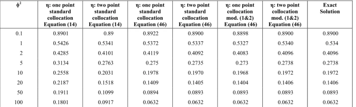
sphere. The results for the case of a slab are given in Table 2 for the effectiveness factor for different φ2. Here Equations (46) and (51) are the same, and only terminal values of u are needed. One point colloca-tion with mod. 1 or 2 and Equacolloca-tion (46) gives rea-sonable results, while exact results are obtained for two-point collocation with mod. 1 or 2.

For the case of a slab, it can be seen from Table 2 that for large Thiele modulus, the results for the stan-dard two-point collocation method using Equation (46) take intermediate values between one and two point collocation with mod. 1 or 2 using Equation (46). The latter is the closest to the exact solution.

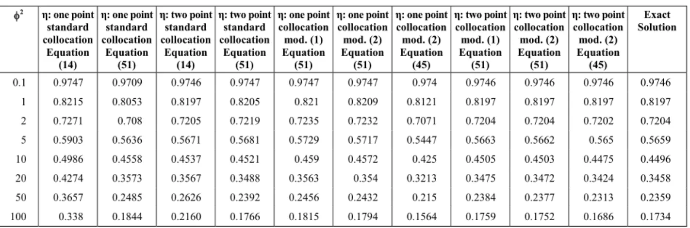
For the case of a cylinder (Table 3), the effective-ness factor calculations require an accurate concen-tration profile. The collocation with mod. 2 using Equation (51) gives the best results. The results for two-point collocation give, on the other hand, a rea-sonable accuracy. It can also be noted that substantial improvement is obtained with standard two-point collocation using Equation (14) over the one-point standard collocation. The same observations are noted for the case of a sphere in Table 4.

Table 2: Effectiveness factor for a 4th order reaction in a slab using different methods.

φ2 _η

: one point standard collocation Equation (14)

η: one point standard collocation Equation (46)

η: one point collocation mod. (1&2) Equation (46)

η: two point collocation mod. (1&2) Equation (46)

0.1 0.8901 0.89 0.8922 0.8900 0.8898 0.8900 0.8900 1 0.5426 0.5341 0.5372 0.5337 0.5327 0.5340 0.534 2 0.4285 0.4101 0.4119 0.4092 0.4083 0.4096 0.4096 5 0.3134 0.2763 0.275 0.2735 0.273 0.2738 0.2738 10 0.2558 0.2031 0.1978 0.1970 0.1968 0.1972 0.1972 20 0.2187 0.1518 0.1409 0.1405 0.1404 0.1406 0.1406 50 0.1911 0.1099 0.0894 0.0893 0.0893 0.0893 0.0893 100 0.1801 0.0917 0.0632 0.0632 0.0632 0.0632 0.0632

Table 3: Effectiveness factor for a 4th order reaction in an infinite cylinder using different methods.

φ2 _η

: one point standard collocation

Equation (14)

η: one point standard collocation

Equation (51)

η: two point standard collocation

Equation (14)

Equation (51)

η: one point collocation mod. (1) Equation

(51)

(45)

η: two point collocation mod. (1) Equation

(51)

(45)

(9)

Table 4: Effectiveness factor for a 4th order reaction in a sphere using different methods.

φ2 _η

: one point standard collocation

Equation (14)

η: one point standard collocation

Equation (51)

Equation (14)

Equation (51)

(51)

(45)

(51)

(45)

0.1 0.9747 0.9709 0.9746 0.9747 0.9747 0.9747 0.974 0.9746 0.9746 0.9746 0.9746 1 0.8215 0.8053 0.8197 0.8205 0.821 0.8209 0.8121 0.8197 0.8197 0.8197 0.8197 2 0.7271 0.708 0.7205 0.7219 0.7235 0.7232 0.7071 0.7204 0.7204 0.7202 0.7204 5 0.5903 0.5636 0.5671 0.5681 0.5729 0.5717 0.5447 0.5663 0.5662 0.565 0.5659 10 0.4986 0.4558 0.4537 0.4521 0.459 0.4572 0.425 0.4505 0.4503 0.4475 0.4496 20 0.4274 0.3573 0.3567 0.3488 0.3563 0.354 0.3213 0.3475 0.3472 0.3424 0.3458 50 0.3657 0.2485 0.2626 0.2392 0.2456 0.2432 0.215 0.2384 0.2377 0.2313 0.2359 100 0.338 0.1844 0.2160 0.1766 0.1815 0.1794 0.1564 0.1759 0.1752 0.1686 0.1734

It can also be seen that, for both the cases of cyl-inder and sphere and for large Thiele modulus, the results for the two-point standard collocation method using Equation (51) give intermediate results be-tween one and two point collocation with mod. 2 and using Equation (51). The latter is the closest to the exact solution.

The use of four-point collocation (not shown) gave exact results. Less accurate results are obtained when using Equation (45) for the evaluation of the effectiveness factor.

CONCLUSIONS

Two modifications are presented to improve the performance of the standard collocation method. In the first modification, we add an extra collocation point to the zeros of Jacobi polynomials at the center of the catalyst particle. The solution is in the form of a higher order polynomial. In the second modifica-tion this polynomial is transformed into a ramodifica-tional function with better accuracy of the solution. When this rational function is used with the proper formula for the effectiveness factor, excellent results are ob-tained. The results are of particular importance to the case of large Thiele modulus where the concentration profile is very steep. Such a case used to be treated by the dead-zone method (Soliman, 1989).

ACKNOWLEDGEMENT

The authors extend their appreciation to the Deanship of Scientific Research at King Saud Uni-versity for funding the work through the research group project No RGP-VPP-188.

REFERENCES

Berrut, J. P., Baltensperger, R. and Mittelmann, H. D., Recent development in barycentric rational interpolation. In: Trends and Applications in Con-structive Approximation. International Series of Numerical Mathematics, 15 27-51 (2005).

Biscaia Junior, E. C., Mansur, M. B., Salum, A. and Castro, R. M. Z., A moving boundary problem and orthogonal collocation in solving a dynamic liquid surfactant membrane model including os-mosis and breakage. Braz. J. Chem. Eng., 18, 163 (2001).

Finlayson, B. A., The Method of Weighted Residuals and Variational Principles. Academic Press, New York (1972).

Finlayson, B. A., Nonlinear Analysis in Chemical Engineering. McGraw-Hill, New York (1980). Soliman, M. A., A modified one point collocation

method for diffusion reaction problems. Chemical Engineering Science 43, 1198 (1988).

Soliman, M. A., Collocation with low order polyno-mials for fast reactions in catalyst particles. Chemical Engineering Science, 44, 1459 (1989). Torres, L. G., Martins, F. J. D. and Bogle, I. D. L.,

Comparison of a reduced order model for packed separation processes and a rigorous nonequilib-rium stage model. Braz. J. Chem. Eng., 17, 915 (2000).

Villadsen, J. V. and Stewart, W. E., Solution of boundary-value problems by orthogonal colloca-tion. Chemical Engineering Science, 22, 1483 (1967).