REM WORKING PAPER SERIES
Self-defeating austerity in Portugal during the Troika’s
economic and financial adjustment programme
José Carlos Coelho
REM Working Paper 0124-2020
April 2020
REM – Research in Economics and Mathematics
Rua Miguel Lúpi 20,1249-078 Lisboa, Portugal
ISSN 2184-108X
Any opinions expressed are those of the authors and not those of REM. Short, up to two paragraphs can be cited provided that full credit is given to the authors.
REM – Research in Economics and Mathematics
Rua Miguel Lupi, 20 1249-078 LISBOA Portugal
Telephone: +351 - 213 925 912 E-mail: rem@iseg.ulisboa.pt https://rem.rc.iseg.ulisboa.pt/
1
Self-defeating austerity in Portugal during the Troika's economic and
financial adjustment programme
April 2020
José Carlos Coelho
ISEG, Lisbon School of Economics & Management – Universidade de Lisboa
jcarlosmcoelho@phd.iseg.ulisboa.pt
Abstract: In 2011, Portugal agreed with the Troika (European Commission, European Central
Bank and International Monetary Fund) to implement an economic and financial assistance programme during the period 2011-2014. One of the objectives of the programme was to guarantee the sustainability of public accounts, by setting targets for reducing the weight of the budget balance on GDP. Between 2010 and 2013, the weight of the budget deficit on GDP decreased by six percentage points. However, in that period, there was a colossal destruction of jobs and the unemployment rate grew by five percentage points. In an Input-Output framework, we show the existence of a negative relationship between the unemployment rate and the budget deficit and we revisit the concept of neutral budget balance proposed by Lopes and Amaral (2017), and also we consider the use of alternative fiscal policies and a mix of fiscal policies. In an empirical application to the Portuguese case, in 2013, we concluded that: (i) the balance of public accounts in that year would imply a very high unemployment rate; (ii) the larger the budget balance in that year, the greater the negative impact on the budget balance in 2014; and (iii) the budget balance actually verified in 2013 had a detrimental effect on the reduction of the budget deficit in 2014.
Keywords: unemployment, budget deficit, self-defeating austerity, Troika, Portugal JEL codes: C67, D57, E24, E62
2 1. Introduction
The Portuguese economy between 1999, with start of euro as single currency in the context of EMU (Economic and Monetary Union) participation, and 2011, with the signature of Economic and Financial Assistance Programme with European Commission, European Central Bank and International Monetary Fund (the Troika), exhibited low economic growth and generated significant internal and external imbalances. In 2007, Olivier Blanchard stated that the Portuguese economy, showing low growth in productivity and GDP per capita, a high budget deficit and a very high external account deficit, faced serious problems (Blanchard, 2007). In the context of EMU, Greece had a similar dynamic, although with budget deficits and external deficits morepronounced. Simultaneously with the occurrence of public accounts deficits and significant external imbalances, the accumulation of high public debts and external debts also happened in these countries.
Between 1999 and 2010, in Portugal, real GDP per capita grew at an average annual rate of 0.7%, gross fixed capital formation as a percentage of GDP decreased from 27.6% to 20.6% and the unemployment rate rose from 4.4% to 10.8%. The average budget balance as percentage of GDP was – 5.4% and the weight of public debt on GDP almost doubled, growing from 54.8% to 100.2%. The chronic and persistent external deficits were particularly high. More specifically, the average weights of external balance of goods and services and current external balance on GDP achieved – 8.4% and – 9.6%, respectively.In effect, the weight of net external debt on GDP has increased fivefold, from 16.3% to 83.3%. The net international investment position as a percentage of GDP, in turn, deteriorated by more than seventy percentage points, from – 35.7% to – 107.2%.
The global financial crisis of 2008 contributed, on the one hand, to the deterioration of the Portuguese economy, which is vulnerable and with structural weaknesses, and, on the other hand, it exposed the internal and external imbalances accumulated until then and precipitated the correction of external deficits. The contagion of the Greek crisis in 2010 was transmitted to Portugal and the country faced liquidity difficulties (with rationed credit and at higher interest rates) in the international sovereign debt markets, and culminated with the signature of the adjustment programme with the Troika.1
On its turn, the adjustment programme negotiated with the Troika in May 2011 was based on a contractionary and pro-cyclical fiscal policy associated with a strongly restrictive income
3 policy, and resulted in a significant fall in domestic demand, in addition to the situation of reversal of external financing occurred in the Portuguese economy, only partially outdated as a result of the aforementioned economic and financial assistance programme. In 2013, and compared to 2010, the programme resulted in a severe recession (GDP at constant 2011 prices decreased by 6.8%), in a colossal destruction of jobs (less 469000 employees), in a high growth of the unemployment rate (with an increase of 5.4 percentage points, having reached 17.5% in the first quarter of 2013), and, in particular, an increase of the youth unemployment rate, which reached the maximum value in 2013, 38.1%, and which are values much higher than those foreseen in the programme adjustment, and in massive emigration (350504 people, 149742 permanent emigrants). The weight of public debt on GDP increased, between 2010 and 2013, more than thirty percentage points, from 100.2% to 131.4%.
Greece, Ireland and Cyprus also negotiated economic and financial adjustment programmes, and in these countries, as well as in Portugal, the effects of fiscal consolidation were recessive, there was an increase of unemployment rates, tax revenues decreased, transfers increased and there was a deterioration of the budget balance and an increase in public debt. The Greek case was the most serious, as the fiscal policy implemented was strongly contractionary and pro-cyclical and generated a vicious cycle of recession and job destruction that had an adverse impact on public finances and, consequently, the weight of public debt on GDP increased significantly. The budgetary consolidation observed was disappointing and the social costs of the measures applied were very large. In this context, it is consensual to say that Greece had an economic depression amplified by the strongly recessive effects of the budgetary austerity measures carried out. These effects undoubtedly demonstrate the self-defeating nature of these same measures, which justifies the fact that some authors have proposed and accepted the expression self-defeating austerity as valid (Chowdhury and Islam, 2012; Skidelsky, 2015). From a macroeconomic perspective, one of the philosophies underlying the economic and financial adjustment programmes applied by the Troika was based on the idea of expansionary austerity, with the expectation of verifying the non-Keynesian effects of fiscal policy (Alesina and Ardagna, 2010). In this case, the multiplier effects associated with fiscal policy instruments are negative. There was also a more moderate view that considered that these multiplier effects were low. However, the experience of the countries where these programmes were implemented, especially in Greece and Portugal, does not corroborate these perspectives. Expansionary austerity did not produce the expected effects and the multiplier effects of fiscal policy proved to be higher than the values that had been initially estimated (Zezza, 2012;
4 Blanchard and Leigh, 2013).2 Thus, the negative effects of the fiscal consolidation policies followed in these countries on employment and the budget balance itself were clearly underestimated, and, with regard to the objective of guaranteeing the sustainability of public accounts, this was strongly threatened and questioned. Nevertheless, in Portugal, the weight of budget deficit on GDP fell 6.3 percentage points, between 2010 and 2013, and the expressive contraction in imports and the increase in exports in this period resulted in a surplus in external accounts.
The multiplier effects of fiscal policy are highest when an economy is in a recession and thus below its level of full employment (De Long and Summers, 2012). Consequently, a fiscal stimulus may be compatible with the reduction of the weight of public debt on GDP (Leão, 2013). Likewise, the adoption of budgetary austerity measures can result in the opposite effect, that is, in the increase of this ratio, as happened with Greece and, to a lesser extent, with Portugal. However, the application of budgetary expansionary measures has adverse effects on the external accounts, with the deterioration of the trade balance and current external balance. The analysis presented in this article is developed in the context of formalizing the structure of the economy through the Leontief model (Input-Output system). The perspective of analysis considered is Keynesian, in which the values of external demand (exports) and the labour force are fixed, the unemployment rate is determined by (endogenous) levels of domestic demand, which is dependent on budgetary options, either through the fixing of a target for the budget balance either by fixing the values of the fiscal policy instrument variables, and imports are the result of the values that these variables assume and, in turn, determine the value of the external deficit (trade deficit, stricto sensu).
The main asset of the IO methodology is the fact that the structural relations established between the productive sectors of economic activity are relatively independent of changes in the economic context and economic policy measures. Therefore, the relations derived from the Leontief model are relatively stable in the short term and the IO methodology is an appropriate tool to determine impacts resulting from shocks, in a framework of comparative static analysis, to compare alternative economic policy options and to proceed the evaluation of macroeconomic projections and policies. In a context of severe economic shocks, technological
2 There is an extensive theoretical and empirical literature, although contradictory, about the multiplier effects of fiscal policy, which discusses and evaluates the dimension of these effects, their pro-cyclical/counter-cyclical character, the possibility of changing their values during periods of consolidation, and its explanatory factors. See, for example, Briotti (2005), Fontana (2009), Spilimbergo et al. (2009), Hebous (2011), Ramey (2011), Batini et al. (2012), Gechert and Will (2012) and Silva et al. (2013).
5 relations are relatively robust. Nevertheless, the IO analysis is not an adequate instrument for making macroeconomic forecasts, and, consequently, the use of this methodology is not recommended for this purpose.
This article makes an empirical application to Portugal, referring to the year 2013, of the macroeconomic and fiscal policy analysis developed in an Input-Output framework. The year 2013 is a relevant year of study, since it is the third year of application of the Troika's Economic and Financial Assistance Programme and for which an analysis based on the intersectoral relations derived from the Leontief model was not carried out. Amaral and Lopes (2017) and Lopes and Amaral (2017), for your side, present empirical results for Portugal relating to 2011 and 2012. Additionally, in 2013, the unemployment rate registered the highest value during the external assistance programme, 16.2%. Therefore, it is considered relevant to ascertain the impact of the increase (reduction) of the budget balance in that year on the employment/unemployment rate and on the budget balance in 2014, through the concept of neutral budget balance proposed by Lopes and Amaral (2017), and the analysis of the possibility of obtaining it using alternative fiscal policies and a mix of fiscal policies.
The structure of the paper is as follows. Section 2 develops the trade-off relationship between the unemployment rate and the budget deficit. Section 3 revisits the concept of neutral budget balance advanced by Lopes and Amaral (2017). Section 4 examines the possibility that the neutral budget balance can be obtained using alternative fiscal policies. Section 5, on its turn, considers the possibility of using a mix of fiscal policies. Section 6 is an empirical application to the Portuguese case in 2013 of the sector-based macroeconomic and fiscal policy relations proposed in the previous sections. Finally, Section 7 presents the conclusions of the paper.
2. The trade-off relation of unemployment rate and budget deficit
Lopes and Amaral (2017) propose the existence of a trade-off relationship between employment and budget balance. In this section, we advance the existence of the trade-off relation of unemployment rate and budget deficit.
The level of total employment, L, is:
L = lC C + lG G + lI I + lE E (1)
Assuming lC, lG, lI, lE as the employment coefficients of private consumption, public consumption, investment and exports, respectively, the previous expression and the expression (A15), C(B) = [n / (1 – nvaC)] (vaG G + vaI I + vaE E + O*) – [n / (1 – nvaC)] B (see in Appendix), the level of total employment, comes:
6
L = lC C(B) + lG G + lI I + lE E L = lC {[n / (1 – nvaC)] (vaG G + vaI I + vaE E + O*) + lG G +
lI I + lE E} – [nlC / (1 – nvaC)] B (2)
Since N is the labour force and u = 1 – L / N is the unemployment rate, then we can write the unemployment rate as a function of the budget balance:
u = 1 – {[(nlC vaG) / (1 – nvaC) + lG] (G / N) + [(nlC vaI) / (1 – nvaC) + lI] (I / N) +
[(nlCvaE) / (1 – nvaC) + lE] (E / N) + [nlC / (1 – nvaC)] (O* / N)} + [nlC / N (1 – nvaC)] B (3)
This equation, after setting the values of exogenous variables, represents the analytical expression of a straight line with a positive slope, where the explanatory variable is B. The positive slope, [nlC / N (1 – nvaC)], which corresponds to the relative value of u in terms of B, shows the existence of a trade-off relationship between the unemployment rate and the budget deficit. The relative value of the budget deficit in terms of the unemployment rate is, in turn, higher when N is higher.
The trade-off equation can be written not only in terms of the absolute value of the budget balance, but also in terms of the relative weight of the budget balance on GDP, Y. Therefore, considering the relative value of the budget balance vis-à-vis GDP, b, and combining the expressions (A15), C(B) = [n / (1 – nvaC)] (vaG G + vaI I + vaE E + O*) – [n / (1 – nvaC)] B, and (A7), Y = vaC C + vaG G + vaI I + vaE E (see in Appendix), and eliminating Y, we obtain:
C(b) = {n [(vaG G + vaI I + vaE E) (1 – b) + O*]} / [1 – nvaC (1 – b)] (4)
The expression analogous to (2) is given by:
L = lC C(b) + lG G + lI I + lE E L = lG G + lI I + lE E + lC{n [(vaG G + vaI I + vaE E) (1 – b) +
O*]} / [1 – nvaC (1 – b)] (5)
Considering N e u, the trade-off equation is:
u = 1 – (lG G + lI I + lE E) / N – (nlC / N) {[(vaG G + vaI I + vaE E) (1 – b) + O*] / [1 – nvaC (1 – b)]} (6)
From the analytical expression of this trade-off equation, we conclude that the relative value of the budget deficit in terms of the unemployment rate is not constant.
Since it is assumed that G, I, E, N, lC, lG, lI, lE are exogenous variables, the trade-off relationship between the unemployment rate and the budget deficit can be studied by analyzing the term:
7 This term corresponds to the relationship between private consumption and the weight of the budget balance on GDP (see expression (4)) and expresses a negative relationship between both variables. As there is a negative relationship between the unemployment rate and private consumption and a negative relationship between private consumption and the weight of the budget balance on GDP, we can conclude that there is a negative relationship between the unemployment rate and the weight of the budget deficit on GDP.
This result expresses, therefore, the existence of a trade-off relationship between the unemployment rate and the weight of the budget deficit on GDP, as evidenced in the expression
(3), u = 1 – {[(nlC vaG) / (1 – nvaC) + lG] (G / N) + [(nlC vaI) / (1 – nvaC) + lI] (I / N) +
[(nlCvaE) / (1 – nvaC) + lE] (E / N) + [nlC / (1 – nvaC)] (O* / N)} + [nlC / N (1 – nvaC)] B.
Additionally, as the term 1 – nvaC (1 – b) is positive, the weight of the budget balance on GDP is less than (1 – nvaC) / nvaC.
3. The neutral budget balance
Lopes and Amaral (2017) propose the concept of neutral budget balance, that is, the budget balance that has no repercussions in the following year. The repercussion occurs in two ways, namely: (i) the change in the total amount of social contributions collected and transfers made by the Government to households, in the form of unemployment benefits, resulting from the variation in the level of unemployment; and (ii) the change in the level of total amount paid for public debt service.
The authors express unemployment as a function of the budget balance:
U = AB + D, (7)
where: A = [nlC / (1 – nvaC)] and D = N – {[(nlC vaG) / (1 – nvaC) + lG] G + [(nlC vaI) / (1 – nvaC) + lI] I + [(nlCvaE) / (1 – nvaC) + lE] E + [nlC / (1 – nvaC)] O*}.
The variation of unemployment come as:
ΔU = AB + D – U-1, (8) where U-1 corresponds to the level of unemployment in the year preceding the reference year. Let be θ the weight per worker on public finances imposed by the existence of unemployed workers, by reducing the amount of social contributions collected and increasing the amount of unemployment benefits paid.
8 The budgetary policy for the following year will be conditioned by the existing level of unemployment, as a result of the budget balance reached in the previous year. This effect, which we can call the unemployment effect, is given by:
– θΔU = – θ (AB + D – U-1) (9) Given i, the expected nominal interest rate, the change in the level of payment of interest on public debt is iB. This effect can be called the interest effect.
The total impact on the budget balance of the following year resulting from the fiscal policy chosen in the reference year is the sum of the unemployment and interest effects. Therefore, the impact value, or total effect, ΔB1, is:
ΔB1 = – θ (AB + D – U-1) + iB (10) The value of the neutral budget balance, BN, is obtained solving the expression ΔB1 = 0 in order to B:
BN = θ (D – U-1) / (i – θA) (11)
Considering the term θ (D – U-1) positive, the neutral budget balance is positive, if i > θA, and negative for i < θA. If i = θA, there is no solution.
Let be U0 and B0 the level of unemployment and the budget balance of the reference year, respectively. As mentioned above, N corresponds to the labour force. The unemployment level can also be written as follows:
U = U0 + N Əu / ƏB ΔB (12)
Based on the expression (3), u = 1 – {[(nlC vaG) / (1 – nvaC) + lG] (G / N) + [(nlC vaI) / (1 – nvaC) + lI] (I / N) + [(nlC vaE) / (1 – nvaC) + lE] (E / N) + [nlC / (1 – nvaC)] (O* / N)} + [nlC / N (1 – nvaC)] B, we see that: Əu / ƏB = [nlC / N (1 – nvaC)].
Then, the previous expression come as:
U = U0 + [nlC / (1 – nvaC)] ΔB (13)
This expression is analogous to (7), U = AB + D.
The expression equivalent to (10), ΔB1 = – θ (AB + D – U-1) + iB, is:
ΔB1 = – θ {U0 + [nlC / (1 – nvaC)] ΔB – U-1} + i (B0 + ΔB) (14) The variation in the budget balance compatible with obtaining the neutral budget balance, ΔBN, is given by:
9 ΔBN = [θ (U0 – U-1) – iB0] / {i – θ [nlC / (1 – nvaC)]} (15) Consequently, the neutral budget balance, BN, is:
BN = B0 + ΔBN = B0 + [θ (U0 – U-1) – iB0] / {i – θ [nlC / (1 – nvaC)]} = θ {(U0 – U-1) – [nlC / (1 – nvaC)] B0} / {i – θ [nlC / (1 – nvaC)]} (16)
The previous expression is analogous to (11), BN = θ (D – U-1) / (i – θA).
The variation of transfers that guarantees the achievement of the neutral budget balance is:
ΔTRN = ƏTR / ƏB ΔBN (17) Based on expression (A20), TR = t (vaG G + vaI I + vaE E) / (1 – nvaC) + [ntvaC / (1 – nvaC) + 1] O* – [ntvaC / (1 – nvaC) + 1] B (see in Appendix), we see that:
ƏTR / ƏB = – [ntvaC / (1 – nvaC) + 1]. Therefore, the previous expression can be written as:
ΔTRN = – [ntvaC / (1 – nvaC) + 1] [θ (U0 – U-1) – iB0] / {i – θ [nlC / (1 – nvaC)]} (18) Finally, the amount of transfers corresponding to the neutral budget balance, TRN, is given by:
TRN = TR0 – [ntvaC / (1 – nvaC) + 1] [θ (U0 – U-1) – iB0] / {i – θ [nlC / (1 – nvaC)]}, (19)
with TR0 corresponding to the amount of transfers in the reference year.
4. The neutral budget balance and the use of alternative fiscal policies
Let be ΔK the variation of one of the available fiscal policy instruments (transfers, public consumption and public investment) in the reference year (in which the fiscal policy is implemented). ϒu,K e αB,K are the multiplier effects of the unemployment rate and the budget balance in relation to the available fiscal policy instrument. As defined above, θ is the weight per worker on public finances imposed by the existence of unemployed workers; i is the expected nominal interest rate; U-1 corresponds to the unemployment level of the previous year to the reference year; U0 e B0 correspond to the unemployment level and the budget balance of the reference year, respectively; and N is the labour force.
Let be the expression below, similar to (14), ΔB1 = – θ {U0 + [nlC / (1 – nvaC)] ΔB – U-1} +
i (B0 + ΔB):
ΔB1 = – θ (U0 + N ϒu,K ΔK – U-1) + i (B0 + αB,K ΔK) (20) This expression allows to determine the variation of one of the available fiscal policy instruments that individually guarantees the neutrality of the fiscal policy, through the adoption
10 of a fiscal policy that has no repercussions in the following year. That is, it allows us obtaining the neutral budget balance:
ΔB1 = – θ (U0 + N ϒu,K ΔKN – U-1) + i (B0 + αB,K ΔKN) = 0 ΔKN = – [iB0 + θ (U-1 – U0)] / (iαB,K – θ N ϒu,K ), (21) where ΔKN refers to the variation of one of the available fiscal policy instruments that, in the reference year, guarantees the achievement of the neutral budget balance.
The neutral budget balance for the reference year, BN, is given by:
BN = B0 + ΔBN = B0 + αB,K ΔKN = B0 – αB,K [iB0 + θ (U-1 – U0)] / (iαB,K – θ N ϒu,K) =
B0 [1 – iαB,K / (iαB,K – θ N ϒu,K)] – [αB,K θ (U-1 – U0)] / (iαB,K – θ N ϒu,K) (22) A crucial aspect of this result lies in the fact that the neutral budget balance is dependent on the fiscal policy instrument used and its different value depending on the instrument used.
The total effect, or impact value, on the budget balance of the following year resulting from the fiscal policy chosen in the reference year, using the available fiscal policy instruments (transfers, public consumption and public investment), is the sum of the unemployment and interest effects. Therefore, the total effect, ΔB1, is, respectively:
ΔB1,TR = – θ (U0 + N ϒu,TR ΔTR – U-1) + i (B0 + αB,TR ΔTR) (23) ΔB1,G = – θ (U0 + N ϒu,G ΔG – U-1) + i (B0 + αB,G ΔG) (24) ΔB1,IPub = – θ (U0 + N ϒu,IPub ΔIPub – U-1) + i (B0 + αB,IPub ΔIPub) (25)
5. The neutral budget balance and the use of a mix of fiscal policies
Unlike the previous section in which we consider the possibility of obtaining the neutral budget balance using alternative fiscal policies (exclusive variation of one of the available fiscal policy instruments, namely, transfers, public consumption and public investment), in this section we consider the possibility to use a mix of fiscal policies, with the simultaneous combination of the three available fiscal policy instruments.
Then, let be the expression below, similar to (20), ΔB1 = – θ (U0 + N ϒu,K ΔK – U-1) +
i (B0 + αB,K ΔK):
ΔB1 = – θ [U0 + N (ϒu,TR ΔTR + ϒu,G ΔG + ϒu,IPub ΔIPub) – U-1] + i (B0 + αB,TR ΔTR + αB,G ΔG +
αB,IPub ΔIPub) (26) As we can see, this expression is an augmented version of the expression (20).
11
Obtaining the neutral budget balance requires the previous expression to be cancelled: ΔB1 = 0.
The neutral budget balance for the reference year, BN, is given by:
BN = B0 + αB,TR ΔTRN + αB,G ΔGN + αB,IPub ΔIPubN (27) Since θ, ϒu,TR, ϒu,G, ϒu,IPub, αB,TR, αB,G and αB,IPub assume fixed values and U0, N, U-1, i and B0 are exogenous (constant) variables, it is necessary to find the values of ΔTR, ΔG and ΔIPub that verify the expression (26), and, consequently, guarantee the neutral budget balance.
The values of ΔTRN, ΔGN and ΔIPubN that guarantee the achievement of the neutral budget balance in the reference year can be determined through an optimization problem of a loss function or economic policy losses, in which the achievement of the neutral budget balance is assumed as a constraint. This optimization problem consists of a problem of minimizing a loss function or losses of economic policy, because, in this context, the economic policy maker intends to minimize deviations from the values of the fiscal policy instrument variables that guarantee the achievement of neutral budget balance vis-à-vis the values they effectively assume in the reference year.
Let be the loss function or economic policy losses thus defined:
FN(.) = (TRN – TR0)2 + (GN – G0)2 + (IPubN – IPub0)2, (28) where: TRN, GN e IPubN respect to the values of transfers, public consumption and public investment that guarantee the achievement of the neutral budget balance in the reference year, respectively; and TR0, G0 e IPub0 are the values of transfers, public consumption and public investment actually verified in the reference year, respectively.
Defining ΔTRN = TRN – TR0, ΔGN = GN – G0 and ΔIPubN = IPubN – IPub0, the loss function or economic policy losses can be written then:
FN(.) = (ΔTRN)2 + (ΔGN)2 + (ΔIPubN)2 (29) The optimization problem described above is as follows:
min FN(.) s.t. ΔB1 = 0
The analytical resolution of this optimization problem can be carried out using the Lagrange Multiplier Method, whose Lagrangean function, LN, is as follows:
LN = (ΔTRN)2 + (ΔGN)2 + (ΔIPubN)2 – λ {– θ [U0 + N (ϒu,TR ΔTRN + ϒu,G ΔGN + ϒu,IPub ΔIPubN) –
12 The first order partial derivatives of LN are:
ƏLN / Ə(ΔTRN)2 = 2 ΔTRN + λ θ N ϒu,TR – λ iαB,TR (31)
ƏLN / Ə(ΔGN)2 = 2 ΔGN + λ θ N ϒu,G – λ iαB,G (32)
ƏLN / Ə(ΔIPubN)2 = 2 ΔIPubN + λ θ N ϒu, IPub – λ iαB,IPub (33)
ƏLN / Əλ = – θ [U0 + N (ϒu,TR ΔTRN + ϒu,G ΔGN + ϒu,IPub ΔIPubN) – U-1] + i (B0 + αB,TR ΔTRN + αB,G ΔGN + αB,IPub ΔIPubN) (34) Solving the first order conditions, we obtain:
ΔTRN = λ (iαB,TR – θ N ϒu,TR) / 2 (35) ΔGN = λ (iαB,G – θ N ϒu,G) / 2 (36) ΔIPubN = λ (iαB,IPub – θ N ϒu,IPub) / 2 (37) Equating the expression (34) to 0 and introducing the previous expressions, it comes that:
λ = 2 [θ (U0 – U-1) – iB0] / [(θ N ϒu,TR)2 + (θ N ϒu,G)2 + (θ N ϒu,IPub)2 + (iαB,TR)2 + (iαB,G)2 + (iαB,IPub)2 – 2 θ N ϒu,TR iαB,TR – 2 θ N ϒu,G iαB,G – 2 θ N ϒu,IPub iαB,IPub] (38) Finally, the optimal values of ΔTRN, ΔGN and ΔIPubN are:
ΔTRN = {(iαB,TR – θ N ϒu,TR) [θ (U0 – U-1) – iB0]} / [(θ N ϒu,TR)2 + (θ N ϒu,G)2 +
(θ N ϒu,IPub)2 + (iαB,TR)2 + (iαB,G)2 + (iαB,IPub)2 – 2 θ N ϒu,TR iαB,TR – 2 θ N ϒu,G iαB,G – 2 θ N ϒu,IPub iαB,IPub] (39)
ΔGN = {(i αB,G – θ N ϒu,G) [θ (U0 – U-1) – i B0]} / [(θ N ϒu,TR)2 + (θ N ϒu,G)2 + (θ N ϒu,IPub)2 + (iαB,TR)2 + (iαB,G)2 + (iαB,IPub)2 – 2 θ N ϒu,TR iαB,TR – 2 θ N ϒu,G iαB,G –
2 θ N ϒu,IPub iαB,IPub] (40)
ΔIPubN = {(iαB,IPub – θ N ϒu,IPub) [θ (U0 – U-1) – iB0]} / [(θ N ϒu,TR)2 + (θ N ϒu,G)2 + (θ N ϒu,IPub)2 + (iαB,TR)2 + (iαB,G)2 + (iαB,IPub)2 – 2 θ N ϒu,TR iαB,TR – 2 θ N ϒu,G iαB,G – 2 θ N ϒu,IPub iαB,IPub] (41)
Given the nature of the fiscal policy instrument variables, it is imperative that: TRN, GN and IPubN ≥ 0.
Considering the previous condition, the maximum values, in module, of ΔTRN, ΔGN and ΔIPubN are TR0, G0 and IPub0.
Based on expression (27), BN = B0 + αB,TR ΔTRN + αB,G ΔGN + αB,IPub ΔIPubN, and in the previous expressions, the neutral budget balance for the reference year, BN, come as:
13
BN = B0 + {[αB,TR (iαB,TR – θ N ϒu,TR) + αB,G (iαB,G – θ N ϒu,G) + αB,IPub (iαB,IPub – θ N ϒu,IPub)] [θ (U0 – U-1) – iB0]} / [(θ N ϒu,TR)2 + (θ N ϒu,G)2 + (θ N ϒu,IPub)2 + (iαB,TR)2 + (iαB,G)2 + (i αB,IPub)2 – 2 θ N ϒu,TR iαB,TR – 2 θ N ϒu,G iαB,G – 2 θ N ϒu,IPub iαB,IPub] (42)
6. Empirical application to Portuguese case in 2013 6.1. Data and basic assumptions
The values of the macroeconomic variables related to the level of economic activity (GDP and its components according to the expenditure approach), the variables related to public finances (budget balance and main revenues and expenses of the Government) and the variables associated with the labour market (labour force, employed population and unemployed population) relatively to Portugal, in 2013, are shown in Tables 1, 2 and 3, respectively, and were taken from INE (the Portuguese Statistical Institute).
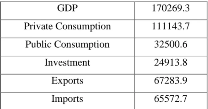
Table 1: Values of GDP and its components according to the expenditure approach
GDP 170269.3 Private Consumption 111143.7 Public Consumption 32500.6 Investment 24913.8 Exports 67283.9 Imports 65572.7
Note: The variables are expressed in millions of euros. Source: INE (2018).
Table 2: Variables related to public finances
Budget Balance – 8245.2
Taxes and Social Contributions 63180.0 Other net Government revenues – 291.6
Public Consumption 32500.6
Public Investment 3848.0
Transfers 34784.9
Note: The variables are expressed in millions of euros. Source: INE (2018).
14 Table 3: Variables associated with the labour market
Labour Force 5284.6
Employed Population 4429.4
Unemployed Population 855.2
Note: The variables are expressed in millions of euros. Source: INE (2018).
From the analysis of Tables 1, 2 and 3, we can see that, in Portugal, in 2013, the external balance was 1711.2 millions of euros; the weight of the external balance on GDP, 1%; the weight of the budget balance on GDP, – 4.8%; and the unemployment rate reached 16.2%.
Based on the values of the relevant macroeconomic variables above, we can also calculate the following values: the available income of private (Yd =141874.2), the average propensity to consume (n = 0.7834), and the average tax rate (t = 0.3711).
Starting from the Input-Output Matrix of National Production for the year 2013 (MPN 2013) made available by INE, and adjusted by the national accounts data, it was possible to calculate the necessary elements to carry out the calibration of the sector-based macroeconomic and fiscal policy relations developed in the previous sections to Portugal, namely the calculation of value added coefficients of the components of final demand. Table 4 present these values.
Table 4: Value added coefficients of the components of final demand
vaC vaG vaI vaE
0.760169 0,760168927
0.905186 0.689701 0.582296
Source: Author´s calculations.
Analyzing Table 4, and as expected, public consumption exhibits the highest value added coefficient, followed by private consumption. This result reflects the fact that public consumption is the component of final demand with less imported content compared to the others. On the contrary, investment and exports are the components of final demand that have the lowest coefficients of added value, which reflects, comparatively, their greater imported content. In particular, the value added coefficient for exports is 0.582296, which means that an additional euro of exports results in an increase on GDP of around 0.58 euros and an increase in imports by 0.42 euros, which constitutes a high value and reflects the external dependence of the productive system of the Portuguese economy.
Based on the employment structure provided by INE (total individuals by industry) and applying it to the total employment in 2013 and to the gross values of sectoral production given
15 by MPN (2013), we determine the employment coefficients of the components of final demand. Table 5 shows these values.
Table 5: Employment coefficients of the components of final demand
lC lG lI lE
0.017754 0.025584 0.017720 0.017585
Source: Author´s calculations.
From the analysis of Table 5, we can see that the highest employment coefficient is that of public consumption and the lowest employment coefficient is that of exports. One aspect to highlight is the fact that the employment coefficients of private consumption, investment and exports are very close.
As exports are expressed in millions of euros and employment in thousands of individuals, the value found for the export employment coefficient (lE = 0.017585) means that the variation of these in one millions of euros can potentially translate into the creation of 17.6 new jobs in the economy.
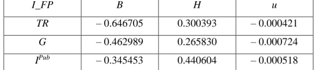
Tables 6 and 7, next, present the multiplier effects of transfers (TR), public consumption (G) and public investment (IPub), fiscal policy instrument variables (I_FP), on budget balance (B), external deficit (H) and unemployment rate (u), and private consumption (C) and GDP (Y), respectively, calculated for Portugal and referring to 2013.
Table 6: Multiplier effects of TR, G and IPub on B, H and u
I_FP B H u
TR – 0.646705 0.300393 – 0.000421
G – 0.462989 0.265830 – 0.000724
IPub – 0.345453 0.440604 – 0.000518
Note: The multiplier effects of u are expressed in percentage points. Source: Author´s calculations.
Table 7: Multiplier effects of TR, G and IPub on C and Y
I_FP C Y
TR 1.252517 0.952125
G 0.713068 1.447238
IPub 0.543318 1.102715
16 6.2. The trade-off relation unemployment rate/budget deficit
The budget deficit/unemployment rate trade-off equations, with the budget deficit expressed in level (B corresponds, by definition, to the symmetrical of the budget deficit) and the budget deficit as a percentage of GDP (b corresponds, by definition, to the symmetrical of the budget deficit as a percentage of GDP), calibrated for Portugal, in 2013, are as follows, respectively:
u(B) = 0.215477+ 0.000007B
u(b) = (0.087157 + 0.544490b) / (0.404487 + 0.595513b)
Since du(B)/dB > 0 and du(b)/db > 0, we conclude, as expected, that the greater the budget deficit and budget deficit as a percentage of GDP, the lower the unemployment rate in the economy, for everything else constant.
Given the values of B and b for Portugal, in 2013, – 8245.2 and – 4.8%, respectively, we obtain the value of the unemployment rate verified in 2013, u = 16.2%.
These equations also allow us to determine, for that year, the unemployment rate corresponding to the budget balance equilibrium scenario, B = 0 (or b = 0). In this case, u would reach 21.5%, 5.3 percentage points above the unemployment rate effectively verified in 2013, and the number of unemployed workers would be 1138707, 36.3% higher than in 2012. The amount of transfers necessary to achieve this scenario would be 22035.4 millions of euros, 33.2% lower than in 2012.
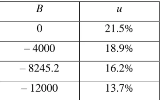
Tables 8 and 9 present combinations of B and u and b and u that verify the trade-off equations
u = f(B) and u = f(b), respectively. These results clearly show the existence of a negative
relationship between unemployment rate and budget deficit and unemployment rate and budget deficit as a percentage of GDP.
Table 8: B and u pairs that verify the trade-off equation u = f(B)
B u
0 21.5%
– 4000 18.9%
– 8245.2 16.2%
– 12000 13.7%
Note: B is expressed in millions of euros. Source: Author´s calculations.
17 Table 9: b and u pairs that verify the trade-off equation u = f(b)
b u
0% 21.5%
– 3% 18.3%
– 4.8% 16.2%
– 6% 14.8%
Source: Author´s calculations.
6.3. The neutral budget balance
The value of the neutral budget balance for Portugal, in 2013, is calculated using the expression (11), presented in section “3. The neutral budget balance”: BN = θ (D – U-1) / (i – θA), or
alternatively, using the expression (16) from the same section: BN = θ {(U0 – U-1) – [nlC / (1 – nvaC)] B0} / {i – θ [nlC / (1 – nvaC)]}.
In 2013, social contributions amounted to 13413.9 millions of euros, corresponding to an employment level of 4429.4 thousand of workers. The amount spent on unemployment benefits was 2725.8 millions of euros for an unemployment level of 855.2 thousand of workers.3 Thus, the average social contributions per worker are 3028.38 euros and the average unemployment benefit is 3187.33 euros. Adding these two amounts, and expressing it in thousands of euros, we obtain the value of θ = 6.215703.
The stock of public debt in 2013 amounted to 219714.8 millions of euros and interest expense was 8258.3 millions of euros. Then, the implicit interest rate of the public debt stock, in that year, was i = 3.8%.
The values A and D of the equation U = AB + D are thus quantified: A = 0.034385 and
D = 1138.707166.
Finally, based on these data, the neutral budget balance for Portugal in 2013 would be – 10692.7 millions of euros, which is higher than the budget balances verified in 2012 and in 2013, – 9529.1 and – 8245.2 millions of euros, respectively. If the budget balance had risen to that amount, we quantify that the external deficit would be – 574.3 and the unemployment rate, 14.6%, with 771016 unemployed workers. GDP would have reached 173872.8 millions of euros, registering a growth of 3.3% compared to 2012 (the nominal GDP growth actually verified in 2013 was 1.1%). Private consumption, on the other hand, would reach 115884.1
3 These values were taken from the Síntese de Execução Orçamental of December 2013, on the website of the Direcção-Geral do Orçamento from Portugal: http://www.dgo.pt.
18 millions of euros. The weights of the budget balance and the external deficit on GDP would be – 6.1% and – 0.3%, respectively. Assuming that this budgetary expansion policy would be implemented using an increase in transfers made by the Government to households, we determine that the value of these would be 38569.6 millions of euros, 16.8% higher than in 2012.
6.4. Effects on the budgetary balance in next year resulting from different budgetary targets in previous year
It is also possible to determine the effect on unemployment as a result of a given fiscal policy implemented in one year and its effects on the budget balance in the following period.
Let be BT the target of the budget balance defined for year 0. The level of unemployment calibrated for that year in function of BT is given by: UT = ABT + D.
It is recalled that the total effect on the budget balance in the following period comes as: ΔB1 = – θ (AB0 + D – U-1) + iB0, where – θ (AB0 + D – U-1) corresponds to unemployment effect
and iB0 corresponds to interest effect.
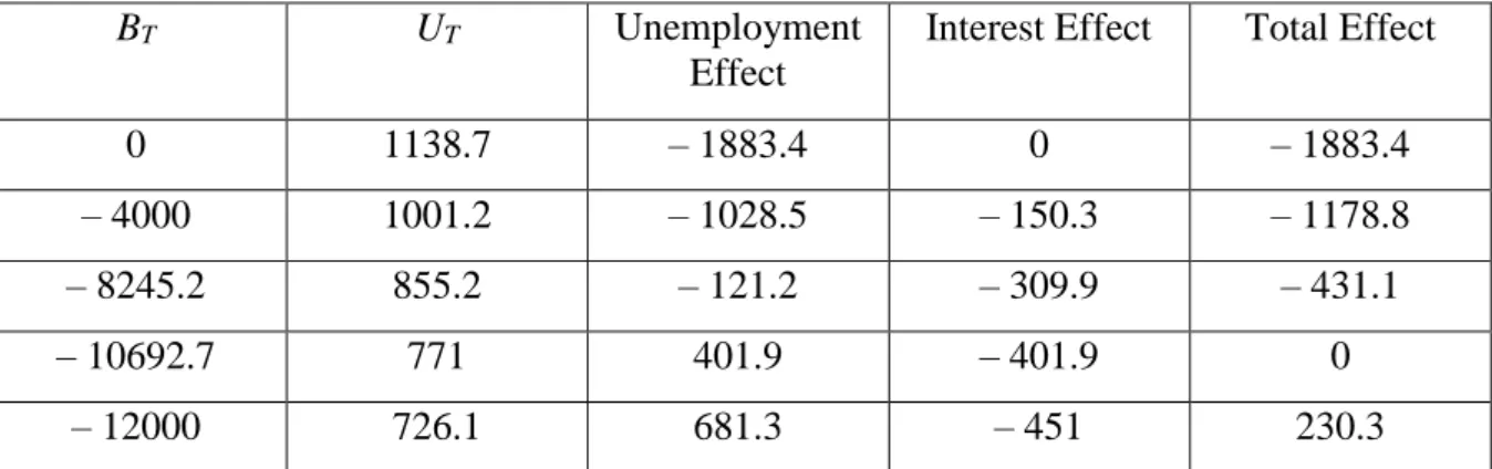
Table 10, below, shows for each alternative BT value, which corresponds to a budget target set in 2013 (year 0) for Portugal, the corresponding unemployment level in that year and the effects on the budget balance (unemployment effect, interest effect and total effect) in 2014.
Table 10: Level of unemployment in 2013 and effects on the budget balance in 2014, resulting from different budget targets in 2013
BT UT Unemployment
Effect
Interest Effect Total Effect
0 1138.7 – 1883.4 0 – 1883.4
– 4000 1001.2 – 1028.5 – 150.3 – 1178.8
– 8245.2 855.2 – 121.2 – 309.9 – 431.1
– 10692.7 771 401.9 – 401.9 0
– 12000 726.1 681.3 – 451 230.3
Notes: (a) UT is expressed in thousands of workers.
(b) BT, Unemployment Effect, Interest Effect and Total Effectare expressed in millions of euros.
Source: Author´s calculations.
As calculated in the previous subsection, the neutral budget balance, in 2013, reaches – 10692.7 millions of euros. To this value corresponds to an unemployment level of 771 thousands of workers, lower than the levels that occurred in 2012 and in 2013, 835.7 and 855.2 thousands of workers, respectively. This value is explained given the expansionary nature of this fiscal policy
19 compared to the fiscal policies followed in 2012 and 2013, which resulted in budget balances of – 9529.1 and – 8245.2 millions of euros, respectively. The effect of this policy on the budget balance in 2014 would be null, by definition.
The budget balance verified in 2013, BT = – 8245.2 millions of euros, corresponds to an unemployment level of 855.2 thousand of workers and a deterioration of the budget balance in 2014 of 431.1 millions of euros.
The fixing of a policy to achieve balance in public accounts, in 2013, would correspond to around 1138.7 thousand of unemployed workers and the deterioration in the balance of public finances, in 2014, of – 1883.4 millions of euros.
For the intermediate values, BT = 0, BT = – 4000 and BT = – 12000, we find that the level of unemployment increases to higher values of B and decreases to lower values of B, which confirms the existence of a trade-off relationship between the level of employment and the budget balance, as shown by Lopes and Amaral (2017). The unemployment effect and the total effect on the budget balance in 2014 are greater for higher values of the budget deficit. The interest effect, in turn, although decreasing to higher values of the budget deficit, is offset by higher values of the unemployment effect.
In sum, more reduced budget deficits translate into higher unemployment levels and result in higher burdens for the Government in the form of unemployment benefit payments and lower collection of taxes and social contributions. This contributes to the deterioration of public finances in the year in which the fiscal policy is implemented and makes the reduction of the budget balance of the following year more difficult. In a scenario of economic recession, as in Portugal, in 2013, this highlights the self-defeating nature of budgetary austerity policies, the so-called self-defeating austerity.
6.5. The neutral budget balance and the use of alternative fiscal policies
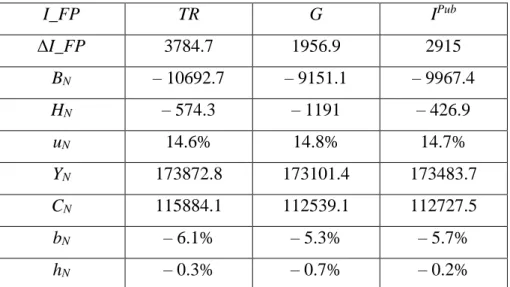
The neutral budget balance can also be obtained using alternative fiscal policies. In this subsection, its value is calibrated for Portugal, in 2013, using this fiscal policy approach. In addition, the values of the remaining relevant macroeconomic variables are determined. Table 11, next, shows, for transfers (TR), public consumption (G) and public investment (IPub), the individual variation of each one of these fiscal policy instrument variables (ΔI_FP) that would guarantee the neutral budget balance in Portugal, in 2013, the neutral budget balance (BN) and the corresponding values of external deficit (HN), unemployment rate (uN), GDP (YN),
20 private consumption (CN), weight of the budget balance on GDP (bN) and weight of the external deficit on GDP (hN).
Table 11: BN related to alternative fiscal policies and corresponding values of HN, uN, YN, CN,
bN and hN I_FP TR G IPub ΔI_FP 3784.7 1956.9 2915 BN – 10692.7 – 9151.1 – 9967.4 HN – 574.3 – 1191 – 426.9 uN 14.6% 14.8% 14.7% YN 173872.8 173101.4 173483.7 CN 115884.1 112539.1 112727.5 bN – 6.1% – 5.3% – 5.7% hN – 0.3% – 0.7% – 0.2%
Note: ΔI_FP, BN, HN, YN and CN are expressed in millions of euros.
Source: Author´s calculations.
From the analysis of Table 11, we observe, as expected, that the value of the neutral budget balance obtained using alternative fiscal policies is different depending on the fiscal policy instrument used for this purpose. The lower neutral budget balance corresponds to a transfers variation of 3784.7 millions of euros compared to its value actually verified in 2013. Also as expected, this value corresponds to the neutral budget balance calculated for Portugal in 2013,
BN = – 10692.7 millions of euros. The lower value of the unemployment rate and the higher values of GDP and private consumption also correspond to this change in transfers. The neutral budget balance corresponding to public consumption takes on the highest value as well as the respective unemployment rate. The lowest values of GDP and private consumption and the highest values of external surplus, weight of the budget balance on GDP and weight of external surplus on GDP refer to public consumption. It should be noted that this is the instrument variable of fiscal policy whose necessary variation that would guarantee the achievement of the neutral budget balance is the smallest, namely, 1956.9 millions of euros. Finally, the lower external surplus and the weight of the external surplus on GDP occur for a change in public investment in 2915 millions of euros.
6.6. The neutral budget balance and the use of a mix of fiscal policies
In this subsection, we determine the neutral budget balance for Portugal, in 2013, using a mix of fiscal policies, with the simultaneous combination of the three available fiscal policy
21 instruments, namely, transfers, public consumption and public investment. The values of the remaining relevant macroeconomic variables are also quantified.
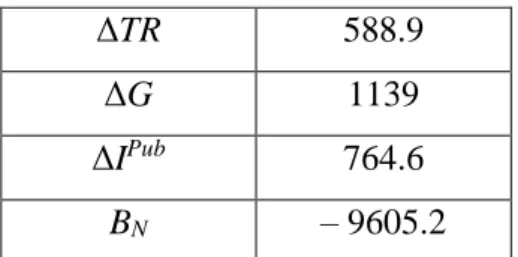
Table 12 presents the variations of transfers, public consumption and public investment would allow reaching neutral budget balance for Portugal, in 2013, using a mix of fiscal policies. Table 12: Values of ΔTR, ΔG and ΔIPub that would allow to reach BN
ΔTR 588.9
ΔG 1139
ΔIPub 764.6
BN – 9605.2
Note: ΔTR, ΔG, ΔIPub and B
N are expressed in millions of euros.
Source: Author´s calculations.
The neutral budget balance in 2013 obtained using a mix of fiscal policies would reach – 9605.2 millions of euros, which represents a deterioration of 16.5% compared to the budget balance actually verified that year, – 8245.2 millions of euros. This value is higher than the neutral budget balance calculated in subsection “6.3. The neutral budget balance”, BN = – 10692.7, but intermediate in relation to the values of the neutral budget balance obtained using alternative fiscal policies (see the information of Table 11).
The neutral budget balance using this fiscal policy approach would be achieved using a simultaneous variation in transfers, public consumption and public investment of 588.9, 1139 and 764.6 millions of euros, respectively.
Table 13 shows the values of external deficit, unemployment rate, GDP, private consumption, weight of the budget balance on GDP and weight of the external deficit on GDP corresponding to the neutral budget balance using a mix of fiscal policies.
From the analysis of Table 13 and comparing their values with the values presented in Table 11, we conclude that the respective values of the remaining relevant macroeconomic variables, assume intermediate values in relation to the determined values in scenarios where recourse to alternative fiscal policies is admitted.
22 Table 13: Values of HN, uN, YN, CN, bN and hN corresponding to BN, obtained using a mix of fiscal policies HN – 894.6 uN 14.7% YN 173321.7 CN 113109 bN – 5.5% hN – 0.5%
Note: HN, YN and CN are expressed in millions of euros.
Source: Author´s calculations. 7. Conclusions
One of the contributions of the paper to the literature consists in establishing the trade-off relationship between the unemployment rate and the budget deficit, following Lopes and Amaral (2017), who advance the existence of a trade-off relationship between employment and budget balance. Considering private consumption endogenous to the functioning of economic activity and dependent on budgetary options, this is, in turn, an employment-inducing variable. More specifically, the variation in transfers made by the Government to households results in a variation in the same direction of private consumption and employment and in a variation in the opposite direction of unemployment rate. Thus, the increase (decrease) in the budget deficit, motivated by the increase (decrease) in transfers made by the Government to households, translates into an increase (decrease) in private consumption and contributes to a decrease (increase) in the unemployment rate.
The trade-off linkage between the unemployment rate and the budget deficit is derived in the context of the formalization of the economy based on the model proposed by Leontief, which considers the technological relations between the productive sectors of economic activity and the relations of final demand. This trade-off linkage is useful, as it allows a relatively expeditious examination of the impact of fiscal reduction (stimulus) measures on the unemployment rate, in the scenario of the exclusive use of transfers.
Through an empirical application to Portugal, in 2013, we concluded, for everything else constant, that obtaining the balance of public accounts in that year would result in an unemployment rate of 21.5%, 5.3 percentage points above the unemployment rate actually verified in 2013. Considering that the budgetary effort would be exclusively based on the
23 reduction of the amount of transfers made by the Government to households, its value would be 33.2% lower than the value of 2012, and the unemployment level would be 36.3% higher. The concept proposed by Lopes and Amaral (2017), and which we have adopted, is the concept of neutral budget balance, which allows us to assess the effects of the reduction of the budget deficit carried out in just one year on the budget balance in the following year. Applying this concept to Portugal, in 2013, we found that the budget balance verified in that year, – 8245.2 millions of euros, had a negative impact of 431.1 millions of euros on the budget balance in 2014. In 2013, the neutral budget balance would be – 10692.7 millions of euros. By setting different fiscal targets for 2013, we concluded that the greater the reduction in the budget balance in one year, the greater the negative impact on the budget balance of the following year, making budgetary consolidation in this year more difficult. Lopes and Amaral (2017) find an identical result for Portugal, which corroborates the self-defeating nature of the budgetary austerity policies applied during the period of external assistance.
Another of the contributions of the paper to the literature is the possibility of obtaining the neutral budget balance using alternative fiscal policies, which considers the exclusive use of each of the available fiscal policy instrument variables, namely, transfers, public consumption and public investment, and also using a mix of fiscal policies. In this approach, the joint use of the available fiscal policy instrument variables is allowed.
Based on the empirical analysis applied to Portugal, in 2013, and using both approaches of fiscal policy, we find that: (i) the value of the neutral budget balance obtained using alternative fiscal policies is different depending on the fiscal policy instrument; (ii) the value of the neutral budget balance obtained with the exclusive use of transfers is identical to the value of the neutral budget balance determined according to the proposal by Lopes and Amaral (2017); and (iii) the value of the neutral budget balance obtained using a mix of fiscal policies is an intermediate value compared to the values of the neutral budget balance obtained using alternative fiscal policies and higher than the value of the neutral budget balance determined according to the proposal by Lopes and Amaral (2017). With regard to the values of the other relevant macroeconomic variables, namely, external deficit, unemployment rate, GDP and private consumption, the values that would occur in the scenario of using a mix of budgetary policies would be intermediate values in relation to the values obtained in scenarios in which alternative fiscal policies are used.
24 Finally, the sector-based macroeconomic and fiscal policy analysis developed can be used to evaluate the Troika's economic and financial adjustment programmes in the cases of Greece, Ireland and Cyprus and to examine the impact of the measures to reduce the budget balance on employment/unemployment rate and on the budget balance of the following year.
Appendix
Basic assumptions and Input-Output relations
In an economy formalized by the Leontief system (see Miller and Blair, 2009, and Amaral and Lopes, 2018, for a more detailed exposition of the model), the basic system is as follows:
X = A X + Y, (A1)
where: X is the (column) vector of the gross production values of n sectors of the economy; Y corresponds to the (column) vector of the final demand; and A is the matrix of technical coefficients.
The system solution is:
X = (I – A)-1 Y, (A2)
where (I – A)-1 is the Leontief inverse matrix of production multipliers, which can be
represented by B, whose generic element, bij, represents the increase in production in sector i resulting from an additional unit of final demand directed to sector j.
The final demand vector can be decomposed into four vectors, corresponding to each of the components of this variable, namely: private consumption (C); public consumption (G); investment (I); and exports (E). Then, it comes:
Y = C+ G + I + E (A3) In this case, the solution of the Leontief system is given by:
X = B (C+ G + I + E) (A4) In this context, the Gross Domestic Product at market prices (GDPmp) results from the sum of gross added value with indirect taxes less subsidies on products and it is calculated as follows:
GDPmp = av B aC C + av B aG G + av BaI I + av BaE E + at B aC C + at B aG G + at BaI I +
at B aE E + at
C C + atG G + atI I + atE E = av B ∑ (aC C + aG G + aI I + aE E) +
at B∑ (aC C + aG G + aI I + aE E) + at
25 where: av is the vector (line) of the value added coefficients of the n sectors (avj = VAj / Xj); aC,
aG, aI, aE are the vertical structures of the components of final demand directed to the productive
sectors; at is the vector (line) of the coefficients of indirect taxes less subsidies on products of
intermediate consumption; atC, atG, atI e atE are the vertical coefficients of indirect taxes less subsidies on products directly attributed to the components of final demand; and C, G, I, E are the values of the components of the final demand. The term av B∑ (aC C + aG G + aI I + aE E)
corresponds to gross value added and the term at B∑ (aC C + aG G + aI I + aE E) + at
C C +
atG G + atI I + atE E corresponds to indirect taxes less subsidies on products.
The value added coefficients of the components of final demand are expressed as:
vaFD = av B aPF + at B aPF + atFD, with FD = C, G, I, E (A6) Therefore, in an economy modellized by IO relations, GDPpm, Y, is given by:
Y = vaC C + vaG G + vaI I + vaE E (A7)
I corresponds to total investment, resulting from the sum of private investment and public
investment (IPriv + IPub).
When the economy is modellized in an IO system (according to the Leontief model) and considering the assumptions previously explained, imports, M, are thus obtained:
M = am B aC C + am B aG G + am BaI I + am B aE E + am
C C + amG G + amI I + amE E =
am B∑ (aC C + aG G + aI I + aE E) + am
C C + amG G + amI I + amE E, (A8) where: am is the vector (line) of the coefficients of the imported inputs; and amC, amG, amI e amE
are the vertical coefficients of imports directly attributed to the components of final demand. From this result, we can express the import coefficients of the components of final demand as well:
mPF = am B aPF + amFD, with FD = C, G, I, E (A9)
Given the equilibrium condition of the IO matrices, PIBpm + M = C + G + I + E, we can conclude that:
mPF = 1 – vaPF (A10)
Consequently, the value of imports made in the economy can be determined as:
26 The relationship between budget balance and external deficit
Following Lopes and Amaral (2017), the budget balance, B, comes as:
B = tY + O – G – IPub – TR, (A12)
where: t corresponds to the average tax rate (t = T / Y), with T meaning the total amount of tax revenues (taxes and social contributions); O are other net Government revenues (including public debt interest); and TR are transfers made by the Government to households.
For simplification, the available income of private, Yd, is equal to Y – tY + TR. Private consumption is a function of Yd: C = nYd, with n representing the average propensity to consume.
With these assumptions, and considering O* = O – G – IPub, C is given by:
C = n (Y + O* – B) (A13)
Using the expression (A7), Y = vaC C + vaG G + vaI I + vaE E, and after some algebraic manipulations, it comes that:
Y(B) = (vaG G + vaI I + vaE E + nvaC O*) / (1 – nvaC) – [nvaC / (1 – nvaC)] B (A14)
From this result, we obtain private consumption as a function of the budget balance:
C(B) = [n / (1 – nvaC)] (vaG G + vaI I + vaE E + O*) – [n / (1 – nvaC)] B (A15)
It should be noted that, in this expression, we consider that the other net revenues of the Government, public consumption and public investment are constant. Therefore, the change in the budget balance results from the change in transfers and their impact on tax revenues. We also consider that private investment and exports are exogenous variables, that is, their values, in the short term, are not dependent on budgetary options by the Government nor do they affect the budget balance.
Considering the expression (A11), M = (1 – vaC) C + (1 – vaG) G + (1 – vaI) I + (1 – vaE) E, and
assuming that private consumption is dependent on budgetary options, the value of imports made in the economy, depending on the budget balance, M(B), can be written as:
M(B) = (1 – vaC) C(B) + (1 – vaG) G + (1 – vaI) I + (1 – vaE) E (A16)
The external deficit can be written as a function of the budget balance, H(B). Then, using the previous expression, it comes:
27
Combining the previous expression with the expression (A15),
C(B) = [n / (1 – nvaC)] (vaG G + vaI I + vaE E + O*) – [n / (1 – nvaC)] B, and after some algebraic manipulations, we have:
H(B) = [n (1 – vaC) / (1 – nvaC)] O* + [(n – 1) vaG / (1 – nvaC) + 1] G + [(n – 1) vaI / (1 – nvaC) + 1] I + vaE [(n – 1) / (1 – nvaC)] E – [n (1 – vaC) / (1 – nvaC)] B (A18)
Assuming the implementation of a fiscal policy that aims to obtain a certain level of the budget balance using transfers, we can determine the amount of transfers compatible with the target set for the budget balance.
As defined above, the budget balance is: B = tY + O*– TR, with O* = O – G – IPub, considered endogenous.
For a given B, comes TR = tY + O* – B. (A19)
Using the previous expression and replacing the expression found for Y in (A14),
Y(B) = (vaG G + vaI I + vaE E + nvaC O*) / (1 – nvaC) – [nvaC / (1 – nvaC)] B, we get TR as a function of B:
TR(B) = t (vaG G + vaI I + vaE E) / (1 – nvaC) + [ntvaC / (1 – nvaC) + 1] O* –
[ntvaC / (1 – nvaC) + 1] B (A20) This expression allows the target of the budget balance to be determined, the amount of transfers
necessary to achieve it, considering that G, I, E and O* are exogenous (constant) variables.
The employment contents of the components of final demand
Let be al the vector (line) of the sectoral employment coefficients, in which each element is the
employment coefficient of sector i, given by: ali = Li / Xi, where Li corresponds to the employment level of sector i; and Xi, to the gross value of production in sector i.
The level of total employment, L, is given by:
L = al X, (A21)
where X is the (column) vector of the gross production values of n sectors of the economy. Given the expression (A4), X = B (C + G + I + E), and since C = aCC,G = aGG, I = aII and
E = aEE, the previous expression can be written as:
L = al B aCC + al B aGG + al B aII + al B aEE (A22)
28
lFD = al B aPF, with FD = C, G, I, E (A23)
The neutral budget balance
The external deficit, the unemployment rate, GDP and private consumption corresponding to the neutral budget balance, HN, uN, YN e CN, respectively, come as:
HN = H0 + ΔHN = H0 + ƏH / ƏB ΔBN (A24)
uN = u0 + ΔuN = u0 + Əu / ƏB ΔBN (A25)
YN = Y0 + ΔYN = Y0 + ƏY / ƏB ΔBN (A26)
CN = C0 + ΔCN = C0 + ƏC / ƏB ΔBN (A27)
H0, u0, Y0 and C0 corresponds to the external deficit, unemployment rate, GDP and private
consumption in the reference year. Considering the expressions (A18), (3), (A14) and (A15), H(B) = [n (1 – vaC) / (1 – nvaC)] O*
+ [(n – 1) vaG / (1 – nvaC) + 1] G + [(n – 1) vaI / (1 – nvaC) + 1] I + vaE [(n – 1) / (1 – nvaC)] E
– [n (1 – vaC) / (1 – nvaC)] B, u(B) = 1 – {[(nlC vaG) / (1 – nvaC) + lG] (G / N) + [(nlC vaI) / (1 – nvaC) + lI] (I / N) + [(nlCvaE) / (1 – nvaC) + lE] (E / N) + [nlC / (1 – nvaC)] (O* / N)} + [nlC / N (1 – nvaC)] B, Y(B) = (vaG G + vaI I + vaE E + nvaC O*) /
(1 – nvaC) – [nvaC / (1 – nvaC)] B, and C(B) = [n / (1 – nvaC)] (vaG G + vaI I + vaE E + O*) – [n / (1 – nvaC)] B, respectively, we have: ƏH / ƏB = – [n (1 – vaC) / (1 – nvaC)],
Əu / ƏB = [nlC / N (1 – nvaC)], ƏY / ƏB = – [nvaC / (1 – nvaC)] and ƏC / ƏB = – [n / (1 – nvaC)]. The values of the external deficit, unemployment rate, GDP and private consumption corresponding to the neutral budget balance, HN, uN, YN e CN, respectively, are given by:
HN = H0 – [n (1 – vaC) / (1 – nvaC)] [θ (U0 – U-1) – iB0] / {i – θ [nlC / (1 – nvaC)] (A28) uN = u0 + [nlC / N (1 – nvaC)] [θ (U0 – U-1) – iB0] / {i – θ [nlC / (1 – nvaC)]} (A29)
YN = Y0 – [nvaC / (1 – nvaC)] [θ (U0 – U-1) – iB0] / {i – θ [nlC / (1 – nvaC)]} (A30) CN = C0 – [n / (1 – nvaC)] [θ (U0 – U-1) – iB0] / {i – θ [nlC / (1 – nvaC)]} (A31)
The neutral budget balance and the use of alternative fiscal policies
In this context, the values of the external deficit, unemployment rate, GDP and private consumption corresponding to the neutral budget balance, HN, uN, YN e CN, respectively, are:
HN = H0 + ΔHN = H0 + ßH,K ΔKN = H0 – ßH,K [iB0 + θ (U-1 – U0)] / (iαB,K – θ N ϒu,K) (A32) uN = u0 + ΔuN = u0 + ϒu,K ΔKN = u0 – ϒu,K [iB0 + θ (U-1 – U0)] / (iαB,K – θ N ϒu,K ) (A33)