The Lisbon stock market from 1903 to 1913 : relationship between returns and macroeconomic variables

(1)

M

ASTER IN

F

INANCE

M

ASTER

’

S

F

INAL

W

ORK

DISSERTATION

The Lisbon stock market from 1903 to 1913: Relationship

between stock return and macroeconomic variables

M

IGUEL

F

RANCISCO

F

ERMOSELLE

S

ILVA

P

EREIRA

(2)

2

The Lisbon stock market from 1903 to 1913:

Relationship between stock return and

macroeconomic variables

M

IGUEL

F

RANCISCO

F

ERMOSELLE

S

ILVA

P

EREIRA

SUPERVISORS:

R

ITA

M

ARTINS DE

S

OUSA

A

MÉLIA

B

RANCO

(3)

3

Abbreviations

GDP Gross Domestic Product

WW I First World War

GNP Gross National Product

T-Bills Treasury Bills

BVL Lisbon Stock Exchange

GHES Gabinete de História Económica e Social

PTE ISEG

Escudo currency

(4)

4

Abstract

The stock markets reactions have been much connected to the political and economic instabilities, leading to changes in the macroeconomic variables. The period of analysis in this research, 1903-1913, is no exception. The situation of political instability in the beginning of 20th century all over Europe was also no exception in Portugal, which during the period of 1903-1913 faced changes in the political governance as a consequence of the assassination of the King.

In what concerns the Lisbon Stock market during this period, the number of companies quoted were not so high and the capitalization (15% of GDP) can be compared with other peripheral stock markets, such as Norway, Italy, Argentina, Chile or Russia. The companies quoted were banks, insurance companies, some industrial companies and, after the end of the 19th century, also colonial companies.

The research question of this master final work is the following: What is the relationship between some macroeconomic variables and the stock returns in the Lisbon Stock Market during the period between 1903 and 1913?

This research question intends to clarify the following aspects:

1. The relation between macroeconomic variables (inflation, GDP, interest rates) and the behaviour of the stock market.

2. The performance of Lisbon Stock market in a period of political and economic instability. The conclusion was that during the period of analysis the rentability was low. In Portugal, between 1903 and 1913, real GDP and inflation had a negative correlation, but inflation and rentability had a positive correlation. This last result – inflation and rentability – was not according theory, but we had during the period low inflation and low rentability. Concerning GDP (nominal and real) this variable had a positive correlation with rentability. The same cannot be conclude when the variable is the industrial GDP. The low number of industrial companies quoted in the Lisbon Stock Exchange can be an explanation for this result. If we consider interest rate, a variable very important for the choice between money and other assets, the conclusion was that real interest rate had a positive effect in the rentability. The opposite with nominal interest rate that had a negative correlation with rentability, as predicted by theory.

(5)

5

Acknowledgments

I would like to thank all the investigators and teachers for their direct and indirect support to my project, recognizing their dedication and work as a great and meaningful help for the consecution of the present investigation project.

I would like also to thank my family and friends for their continuous support, incentives and understanding along the period of time this project took place.

(6)

6 Table of Contents

List of Tables and Figures

Pages

Tables:

Table 1: Description of the different hypothesis 22

Table 2: Monthly index Rentability 27

Table 3: Annual index Rentability 28

Table 4: Relation between inflation and rentability 30

Table 5: Relation between nominal GDP and rentability 31

Table 6: Relation between nominal interest rate and rentability 32

Table 7: Relation between industrial growth (industrial GDP) and rentability 33

Table 8: Relation between real industrial GDP and rentability 34

Table 9: Relation between real industrial GDP and rentability 35

Table 10: Relation between real interest rate and rentability 36

Table 11: Relation between Real GDP and inflation 37

Table I: Economic development indicators 42

Table II: Nominal GDP growth in Percentage (1890-1913) 43

Table III: Nominal public debts in Europe in millions of national currency (1890-1913) 44

Table IV: Short-term nominal interest rates (%) (1890-1913) 45

Table V: The exchange rate (unit: Escudo) 46

Table VI: Inflation rate between (1891-1913) 47

Table VII: Real interest rate (1892-1913) 48

Table VIII: Growth rate of industrial production (1890-1913) 49

Table IX: Real GDP growth (1892-1913) 50

Table X: Lisbon stock market (1880-1910) 50

Table XI: BVL sectorial distribution (number of companies) 51

Table XII: BVL listed companies 51

Table XIII: Lisbon Stock Exchange 52

Figures: Figure 1: Monthly Lisbon Stock Index returns 27

(8)

8

Chapter 1 – Introduction

The stock markets reactions have been much connected to the political and economic instabilities, leading to changes in the macroeconomic variables. The period of analysis in this research, 1903-1913, is no exception. The situation of political instability in the beginning of 20th_{century all over}

Europe was also no exception in Portugal, which during the period of 1903-1913 faced changes in the political governance as a consequence of the assassination of the King.

From the economical point of view, Portugal could be considered a country with economic backwardness compared to the major economies in Europe, like France, Germany, United Kingdom or even the Austro-Hungarian Empire. This is somehow explained by the fact that a great percentage of the population was still living in small villages dedicated to agriculture production. Besides that, the communication between cities in Portugal was underdeveloped making it difficult even between the two major cities like Porto or Lisbon, not to mention other cities.

In what concerns the Lisbon Stock market during this period, the number of companies quoted were not so high and the capitalization (15% of GDP) can be compared with other peripheral stock markets, such as Norway, Italy, Argentina, Chile or Russia (Rajan, Zingales, 2003). The companies quoted were banks, insurance companies, some industrial companies and, after the end of the 19th century, also colonial companies.

In this master final work will be done an analysis to some macroeconomic variables, like inflation and interest rates, and perceive how they interact with each other as well as the impact of these macroeconomic variables in the rentability of the Lisbon Stock market. The literature review will be done by builds on insights from some international literature like Eugene Fama, Robert Mundell, and Robert Roll, who explain the stock reactions to changes in some macroeconomic variables.

The research question of this master final work is the following: What is the relationship between some macroeconomic variables and the stock returns in the Lisbon Stock Market during the period between 1903 and 1913?

(9)

9

This research question intends to clarify the following aspects:

1. The relation between macroeconomic variables (inflation, GDP, interest rates) and the behavior of the stock market.

2. The performance of Lisbon Stock market in a period of political and economic instability.

To have a clear-cut general assessment of macroeconomic variables in stock markets, it was assumed that the correlation between macroeconomic variables and stock return is similar in minor and major stock markets like the stock markets of United States of America, United Kingdom or Germany.

In this master final work it is assumed that the correlation between macroeconomic variables and stock returns can be explained by changes on the macroeconomic factors but there are other factors, such as arbitrage opportunities, that were not taken into consideration in this master final work due to lack of information about this topic for the period between 1903 and 1913.

This research is based in the stock market quotations that were provided by the GHES-ISEG/CSG with the research project Capital Markets, 1837-1913.The time span of our analysis is between 1903 and 1913. The choice of this period is related to the great political instability that the World and specially Europe was facing during this period just before the beginning of World War I. Although there is data from a period before the decade 1903-1913 the choice of narrowing the time span of this master final work can be related with all the aspects referred previously that make this decade the most appealing decade for studying the Lisbon Stock Market. The methodology that will be used to test the different hypothesis is a two-paired sample t-test and the analysis will be done on the Pearson correlation.

This master final work has seven different chapters which will be summary described in the following paragraphs. After this chapter one, in chapter two will do a literature review about the behaviour of stock returns and macroeconomic variables. In chapter three there is a description of

the Portuguese social and economic situation in the beginning of the 20th century. In the following

chapter we will develop a description of the Lisbon stock market showing its relevance in the Portuguese economy. In the fifth chapter there is a description of the methodology used in this master final work as well as the hypothesis to be tested. In chapter six we will present the results

(10)

10

of the hypothesis with an analysis and comparison with the major theories described in chapter two. In the seventh chapter we present the conclusions of this master final work as well as some recommendations for future analysis.

(11)

11

Chapter 2 – Literature Review

The purpose of this master’s final work is to better understand the impact of some macroeconomic variables in the Lisbon Stock Exchange during the period between 1903 and 1913.There are some points from the literature referred that should be taken into consideration when we analyze the Portuguese stock market. The first point is that the great majority of these studies were done in the period after the WW I. The second one is that the evidences obtained from the main markets such as UK, USA or Germany may not be applicable on the peripheral economies.

In this chapter we present some literature review considering the relationship between some economic variables, such as, inflation, real activity, interest rates, and stock returns.

2.1 Impact of inflation in stock returns

In this point there are two variables to consider which are the expected inflation and the unexpected inflation.

As it is referred on the Farlex financial dictionary (2015) the expected inflation is the expectation of all stakeholders about the current and also future inflation, but this expectation may not be rational. As a consequence this may affect how the market reacts to changes in the target interest rate. According Farlex financial dictionary (2015) unexpected inflation happens every time the inflation rate is higher than the inflation predicted by the specialists.

As Fama (1977) stated and supported by Kessel (1956) there is a positive correlation between unexpected inflation and stock returns in companies that can be considered as net debtors. Theoretically a company with more long-term paying fixed agreements than the amount of fixed receiving agreements tend to have a positive correlation. Although, it is also stated that in the real world it is difficult to analyze this correlation, because other factors have to be considered, such as, the relation between the purchase of labour, raw materials, and capital with the borrowing/selling of contracts. For companies that can be considered as net creditors, the unexpected inflation shows to have a negative correlation with stock returns.

Considering expected inflation, the correlation with stock returns is negative as it is stated by Fama (1977) and supported by a set of different authors, such as, Nelson (1976), Linter (1975) or Jaffe

(12)

12

and Mandelker (1976). Fama was unable to identify the economic origins of this phenomena and only considered some hypothetical explanations. The first explanation is that an unidentified macroeconomics phenomenon might cause equilibrium expected on real returns to stocks to be negatively related to expected inflation rates. The second explanation pointed out is that markets can be inefficient in impounding available information about future inflation into stock prices. In what concerns stock returns it is also important to consider Lee (1992). According to this author, the correlation between nominal stock returns and inflation is defined as weakly negative and the correlation between inflation and real stock returns can be defined as mildly negative. These conclusions are the opposite of the correlation defined by Fisher (1930) where the correlation between nominal stock returns and inflation is defined as weakly positive and the correlation between inflation and real stock returns can be defined mildly positive.

According to Lee (1992) these different conclusions can be justified by the period under analysis. The negative correlation between stocks returns and inflation, observed during the postwar period, may not be a reliable relation for future analysis and for the purpose of prediction.

2.2 Relation among real activity and stock returns

In Fama (1981), the focus of analysis is to explain the negative relationship between stock returns and inflation as a consequence of proxy effects, such as the real activity. Also in his study Fama (1981) reaches the conclusion that there is a consistent evidence of negative relations between inflation and real activity which is only possible to understand considering always the context of

Money Demand Theory and the Quantity Theory of Money1_.

In the proxy effect scenario the measures of real activity have more weight and should be more considered than measures of inflation when these two variables are used as explanatory variables in stock returns regressions. When analyzing data collected in a monthly, quarterly and annual base the growth rate of money and real activity eliminate the negative correlation between real

1_{The Money Demand Theory can be explained by the total quantity of money and the total amount of spending on final goods and}

services produced in an economy (Fisher, 1930). The Quantity Theory of Money sets a direct relation between the quantity of money in an economy and the level of prices of goods and services. So, if the amount of money doubles will have as a consequence that prices will double causing inflation (Thornton, 1802).

(13)

13

stock and expected inflation rate. Analyzing also annual stock returns regressions and comparing the unexpected inflation rate with future real activity, it is possible to conclude that the unexpected inflation loses its explanatory power.

Fama (1981) stated, that this theory leaves the author without any logical economic background to explain what happened for the decline of stocks returns during the post-1953 period.

Lee (1992) also analyzes the correlation between the real activity and the stock return and concludes that there is a positive correlation between stock returns and the growth in industrial production. According to the author this gives support to the point that stock returns anticipates upward movements in the growth of industrial production. The author determines that the correlation between inflation and the subsequent growth in industrial production is negative. Considering the relation between nominal interest rate and industrial production growth, the correlation is also negative. When there is a raise in the nominal interest rate as a consequence of inflationary expectations this will be associated with a lower growth in industrial production. When the analysis is with the real interest rate and the growth in industrial production with real stock returns, the conclusion is that they are positively associated, which, according to the author, is a totally different result from the one obtained by Mundell (1963) who stated that real returns on financial assets were negatively related to real activity.

2.3 Relation among interest rates and stock returns

As stated by Geske and Roll (1983) the negative relation between the short term interest rate, the changes in short-term interest rate, unexpected inflation and stock returns are a consequence of fiscal and monetary policies. Although for the authors the relation between changes in short-term interest rate and stock returns and the relation between unexpected inflation and stock returns are two methods that at the end measure the same thing.

According to Geske and Roll (1983) theory, if there is a positive or negative random event that has an impact on stock returns, it will affect positively or negatively employment as well as the corporate earnings of a set of companies. As a consequence of lower (or higher) corporate earnings there is a reduction (or rise) on corporate and personal tax revenues, but governments take their time to accommodate their expenditures to the changes in the revenue and during this period it is

(14)

14

possible to observe an increase (or decrease) in the treasury’s deficit. Since there is an increase (or decrease) in the treasury’s deficit and as a response to that deficit the treasury starts increasing (or decreasing), the borrowing from the public. The Central Bank starts purchasing part of the change in treasury debt at the same time and eventually it is paid for that by expanding (or contracting) the growth rate of base money.

As a consequence of the expansion (contraction), Geske and Roll (1983) consider that, there is induced inflation since there is a change in growth rate of money base. As expected, the rational investors will realize that any random event that is signaled by the stock market have, as trigger, this monetary and fiscal response. The rational investor will change the prices of short-term securities. At the same time the stock returns change their behaviour having as a consequence an increase (or decrease) deficit triggered by any random event. This event is expected to be monitorized by the Central Bank and so the treasury will increase (or decrease) the supply of debt securities that would also cause an increase (or decrease) in the real interest rate. Investors will understand if a particular stock return will mean a change in real rates, in expected inflation or a mix of both and, regardless the percentage of real growth rate and expected inflation, have as a consequence a change in the nominal interest rate.

As stated by Geske and Roll (1983) there are other studies which state the short-term interest rate has a negative correlation with stock returns. But the conclusions of those studies can be influenced by the methodology used.

Considering the correlation between nominal interest rates and inflation, as it is stated by Lee (1992), it is strongly positive in all data observed and analyzed, being this result equal to the results reached by Fisher (1930) in his paper. In what concerns real interest rate and inflation, the author reaches the conclusion that in this point there is a negative correlation, which again, is in accordance with the findings of Fama and Gibbons (1984).

2.4 Relations among monetary sector and stock returns

As it is stated by Kaul, (1987) as initial hypothesis, the cause for the negative correlation between stock returns and inflation, during the period after the Second World War, had as explanation a set of factors as, a combination of money demand and counter-cycle money supply effects. If money

(15)

15

demand had a pro-cyclical monetary response the correlation between stock returns and inflation would be insignificant or even positive.

In a study for different industrialized countries, USA, UK, Canada and Germany, there was a correlation in three of them which indicates that the negative correlation between inflation and real activity was reinforced by counter-cyclical monetary responses implemented by the monetary authorities.

(16)

16

Chapter 3 – Portugal at the beginning of 20

th

_century

3.1 Political framework

The political environment in Portugal at the end of the 19th century and beginning of the 20th century was one of the most controversial in its history, as Portugal went through three different political regimes during this period.

The first political regime was a representative monarchy with a Parliament that lasted until April 1907. Between April 1907 and February 1908 the political regime can be described as a dictatorship under the aegis of king D. Carlos I, led by João Franco. This dictatorship policy lead

to a dramatic event for the Portuguese Monarchy on February, 1st_{1908, after several months of}

planning, as king D.Carlos I and his older son Prince D. Luís Filipe were killed being his younger son D.Manuel II named king after that event. Between February 1908 and October 1910, D.

Manuel II ruled Portugal. Although all the changing efforts carried out by the king, Portuguese

Monarchy was no longer supported by the people and on October 10th 1910 after a political revolution Portugal became a republic.

The first Republic period in Portugal was a political turmoil period due to internal instability and also due to the political instability across Europe, which would culminate in the First World War. During this period Portugal had a great financial and economic instability which somehow was affected by the European instability. But the main reason for this instability is created inside, as between 1910 and 1913 Portugal had four different governments and the maximum period of a continuous governance lasted one year.

3.2 Economic framework

As it is stated by Reis (1992) the beginning of the 20th century shows some points of industrialization although this industrialization, when compared with other countries in Europe, like UK and Germany, can only be considered as insufficient and inefficient. At the beginning of the 20th century the Portuguese agriculture had more weight in the Portuguese gross domestic product (GDP) than industry. Several explanations can be advanced for this economic structure (Reis, 1992). First of all, a small internal market based on a backward agrarian sector. Second was

(17)

17

a social environment with a weak bourgeoisie. Third a shortage of capital and credit was difficult to get and expensive, particularly for industrial purposes. Fourth the lack of education at elementary and technical level. Finally, compared to most industrialized countries in Europe, Portuguese industrialization was also inefficient due to the large proportion of raw materials used in the industry in this period which needed to be imported, turning the production of these goods in Portugal expensive. The only positive Portuguese industry feature in this period was the low cost of the labour, but surprisingly, according to Reis (1992), this point had a relative low importance although it represented one of the major costs for the industry in that period.

One of the points referred by Reis (1992) is that the growth of the Portuguese GDP between 1891 and 1914 was really small due to all political and economic instability. The growth in the industrial sector observed during this period was higher than the average growth of GDP and especially on the canned food industry, cork industry, chemical industry and modern heavy industry. The service sector also grew at a higher pace than GDP growth, being the transportation service, health service, communication service and education service the ones that grew more during this period.

To get a better idea of the previous two paragraphs in appendix (table I) there is a comparison of

consumption and the development of the terrestrial infrastructures at the beginning of 20th century

(1906) between Portugal and Europe.

Considering Costa et al (2012) during this period the Portuguese government was constantly in deficit, which meant that a proportion of the available capital for investment was spent in interest and so a reduction of capital available for public spending and investment.

As a consequence, during this period it is possible to observe that the Portuguese government, besides having consecutive deficits, tried to guide the Portuguese society towards capitalism. Several measures were taken during this period by the Portuguese government, like increasing the investment spending, implementation of some taxation benefits, making contracted transfers with private agents for the pursuit of public interest projects or even the role of the state helping private companies to reach international capital markets, as it is referred by Gerchenkron (1962).

To get a better picture of the Public debt of Portugal the appendix reveals that Portugal had consecutive deficits, although during the period between 1900 and 1913 there is a reduction in deficit and debt. In table III there is a comparison between the Portuguese situation and the most

(18)

18

developed countries in Europe for this period and it is possible to observe that Portugal is one of the countries with higher debt burden.

According to O´Rourke and Williamson (1999) although all efforts done by the Portuguese government to increase the living standards, this period is also characterized by a constant flow of migration to colonies and other countries in Europe and America. According to those authors the cause of the economic backwardness of Portugal and Spain, compared to other European countries, is a consequence of their weak industrial production to face the open market, being prisoners of very strong customs policies, creating a special protectionism to domestic industry.

3.3. The Portuguese financial crisis of 1891

During the second half of the 19th_{century, Portugal faced the big boost of construction of}

infrastructure financed by public debt. As the economic growth was weak the government expenses were higher than the revenue obtained by collecting taxes and as consequence the debt increased. The second problem was the lack of markets’ confidence on the Portuguese capacity to pay the debt and so the demand for Portuguese T-bill or bonds was really small. At last the political instability did not allow to increase taxes in order to try to balance the unbalanced public expenditure. As a consequence, at the end of 1880 the public debt was near 80% of GDP and the interests paid in T-bills and bonds represented 50% of the tax revenues.

In 1892 Portugal faced a partial bankruptcy as a consequence of the financial instability created by an overspending during several years and also because of two different episodes. The first episode was that Brazil faced some instability, which meant that the Portuguese emigrants living there stopped sending remittances to Portugal, which was an important financial source to the Portuguese government in order to balance somehow the unbalanced current expenses. The second event was the problem with the Baring Brother bank, which financially supported the Portuguese government, via buying T-bills, every year.

In table IV there is a comparison between Portugal and the most developed countries in what concerns interest rates for short-term loans and it is possible to observe that Portugal was one of the countries with higher interest rates.

(19)

19

3.4 Exchange rate and inflation rate

During 1891 crisis the Portuguese government used the Bank of Portugal to finance itself, since the Baring Brother bank could no longer finance the Portuguese government. It was during this crisis that the Banco de Portugal became the only bank authorised to printout currency and so the supply of money suffered a total change.

Portugal run out the gold standard and the currency unit depreciate in the exchange market. At the

beginning of the 20th _{century the parity between Portuguese currency and Pounds was less than a}

fifth of the initial defined and between 1905 and 1911 the parity was between 4$582 and 5$199. After 1910 there was an important change the introduction of a new curreny, the escudo, which was equivalent to 1000 reís. The escudo currency was defined according to gold standard being the value of escudo equal to 1,625g of gold. After 1911 there was a currency devaluation until the WW I, being its value 5$235 as it is possible to observe in appendix table V.

The inflation rate during the period between 1891 and the WW I was not too high and using a price index of 1914 as standard the price variation goes from 0.83 in 1891 to 1.01 in 1913 as it is possible to observe in appendix table VI.

(20)

20

Chapter 4 – The Lisbon Stock Exchange

The analysis of the Lisbon Stock Exchange (BVL) is going to be done via a set of indicators which include the size, composition, dynamics and liquidity of the market.

The role of the stock market, as a way for companies to finance themselves, increases during this period and an example of this is the presence of new sectors such as mining, railways and utilities.

4.1. Size, composition and dynamics

According to Branco, Neves and Sousa (2015) the size of the stock market can be measure by the number of listed companies together with the amount of their paid-up capital.

In table X it is possible to observe an increase of 31% in the number of listed companies in BVL during the period between 1880 and 1910. Considering the share capital, it is possible to observe an increase of 40.6% and the ratio between the share capital of listed companies and the Portuguese GDP increased 1.7%. The results show that before the WWI the BVL number of companies was higher than in 1880 and the market registered more activity with higher values of total paid-up capital. As Branco, Neves and Sousa (2015) this evolution was not a linear one as the market faced moments of greater dynamism and a period of slump, being 1890 the year of the turning point as it was the year that had the highest number of listed companies and the highest weight share capital to GDP (15%).

In table XI it is possible to observe that the sectorial distribution has not suffered big changes in terms of paid-up capital. In a deeper analysis it is possible to observe that the number of companies varied and transports and banking sectors have higher weight, for almost the entire period. At the beginning of the 20th century the colonial companies increased their importance in the Lisbon Stock Market, while the banking sector decreased as a consequence of the financial problems they were facing. At the beginning of the 20th century the banking, transportation and colonial companies represented 80% of share capital and listed companies in BVL.

(21)

21

4.2 Liquidity

The last indicator of this analysis is liquidity. According Branco, Neves and Sousa (2015) this variable is analyzed via a proxy of the number of days with transaction by company, since there is no information about the volume of transactions, only about prices.

The study of liquidity allows a certain understanding of how savings were or not diverted to productive ventures. Analyzing table XII and stating Branco, Neves and Sousa (2015) the number of companies with transactions increased between 1870 and 1910 in general. This evolution followed trends that were observed. In this case the number of listed companies registered an increase until 1890, followed by a decrease during the first half of the 1890, recovering from then until the end of the period.

However, if we consider the percentage of companies with transactions, the disparities in proportion with listed companies holding shares is very unstable, being the range between 38% and 74% and if we restrict the sample for companies with transactions in more than ten per cent of days the range changes to a level between 13% and 36%. These figures point out that the Lisbon Stock Exchange was a low liquidity market.

(22)

22

Chapter 5 – Hypothesis and Methodology

5.1 Hypothesis and Methodology

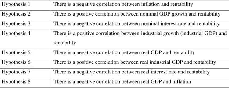
In this research we developed an analysis to the behaviour of stock returns and the relationship with some macroeconomic variables, taking into account the period between 1903 and 1913. Considering the objectives of this research and the literature review, we can regard eight different sets of hypothesis.

Table 1: Description of the different hypothesis

Hypothesis 1 There is a negative correlation between inflation and rentability

Hypothesis 2 There is a positive correlation between nominal GDP growth and rentability

Hypothesis 3 There is a negative correlation between nominal interest rate and rentability

Hypothesis 4 There is a positive correlation between industrial growth (industrial GDP) and

rentability

Hypothesis 5 There is a negative correlation between real GDP and rentability

Hypothesis 6 There is a positive correlation between real industrial GDP and rentability

Hypothesis 7 There is a negative correlation between real interest rate and rentability

Hypothesis 8 There is a negative correlation between real GDP and inflation

Source: Own elaboration

The stock market quotations and the General Index were provided by the GHES-ISEG/CSG with the research project Capital Markets, 1837-1913. The stock quotations were done in a daily basis between 1903 and 1913 and in a quarterly base before that. The time span of our analysis is between 1903 and 1913.

Some assumptions were taken into consideration to construct the General Index (table XIII). First of all, the consideration of only the last quotation of each month for each company. The second assumption was for the composition of BVL, considering only companies which, in each year, had at least transactions/quotation in one fifth of the stock market trading days. The third assumption was that for every quotation there is a transaction price and this was the value for the

(23)

23

quotation of a share. If there was no transaction price an average between the ask price and the bid price was assumed, following this way the recommendation of Ulrich (1905) applying a bid-ask spread.

The next procedure was the calculation of rentability of the Lisbon Stock Exchange as well as volatility.

According to Hull (2008), in order to calculate the rentability of a stock index it is necessary, in the first place, to define the number of observations n+1 and in the second place the quotations Li,

with i = 1, 2,…,n being i days, months or years, to get the rentability via the following formula:

R = 𝑙𝑛( 𝐿𝑖

𝐿 𝑖−1) for i = 1; 2; 3;…; n

To determine if the stock market had a regular stock return during the period between 1903 and 1913 we use the standard deviation and the formula is:

𝜎 = √1

𝑛∑ (𝑥𝑖 − 𝜇) 2 𝑛

𝑖=1 where, 𝜇 is the mean and n is the size of the sample

For testing the hypothesis it is considered a T-test paired two sample for means. The concept behind the T-test consists of a sample of matched pairs of similar units or one group of units that has been tested twice. According to McDonald (2014) the T-test two sample for means has its basis on a matched-pair sample, since it is the result of an unpaired sample that is subsequently used to form a paired sample, obtained by using additional variables that are measured along with the variable of interest. The matching happens by the identification pairs of values consisting of one observation from each two samples, where the pair is similar in terms of other measured variable. Normally this approach is used to reduce or eliminate the impact of confounding factors.

(24)

24

The formula of the t-test is:

𝑋̅ − 𝜇 ( 𝜎 √𝑛) ( 𝑠 √𝑛) Where,

𝑋̅ = is the sample mean 𝑛 = is the sample size

s = ratio of sample standard deviation over population 𝜎 = is the population standard deviation of data 𝜇 = is the population mean

As stated by McDonald (2014), the Pearson coefficient ranges from -1 to 1. A value of 1 implies that a linear equation describes the relation between X and Y perfectly, with all data points lying on a line for which Y increases as X increases. A value of -1 implies that all data points lie for which Y decreases as X increases. A value 0 implies that there is no linear correlation.

More generally note that (Yi-𝑌̅) (Xi-𝑋̅) is positive if Xi and Yi lie on the same side of their

respective means. Thus the correlation coefficient is positive if Xi and Yi tend to be simultaneously

less than their respective means, the correlation coefficient is negative if Xi and Yi tend to lie on

opposite side of their respective means. Moreover, the stronger either tendency is the larger is the absolute value of the correlation coefficient.

For testing these hypothesis there is some data to consider:

1. To test the first hypothesis there is a need to consider the inflation rate (table VI) which was provided by Valério (2001) what concerns price index and own elaboration for inflation rate and general index return (table XIII) which was provided by GHES-ISEG and own elaboration.

(25)

25

2. To test the second hypothesis there is a need to consider the nominal GDP (table II) which was provided by Flandreau, Zumer (). As well as the table general index return (table XIII) which was provided by GHES-ISEG and own elaboration.

3. To test the third hypothesis there is a need to consider the short-term nominal interest rate (table IV) which was provided by Flandreau, Zummer (2004). As well as the table general index return (table XIII) which was provided by GHES-ISEG and own elaboration.

4. To test the forth hypothesis there is as need to consider the growth rate of industrial production (table VIII) which was provided by Lains (1990). As well as the table general index return (table XIII) which was provided by GHES-ISEG and own elaboration.

5. For testing the fifth hypothesis there is a need to consider the real GDP growth (table IX) which was provided by Lains (1990). As well as the table general index return (table XIII) which was provided by GHES-ISEG and own elaboration.

6. For testing the sixth hypothesis there is a need to consider the growth rate of industrial production GDP (table VIII) which was provided by Lains (1990). As well as the table general index return (table XIII) which was provided by GHES-ISEG and own elaboration

7. For testing the seventh hypothesis there is a need to consider the real interest rate (table VII) which was provided by own elaboration. As well as the table general index return (table XIII) which was provided by GHES-ISEG and own elaboration.

8. To test the eighth hypothesis there is a need to consider the inflation rate (table VI) which was provided by Valério (2001) in what concerns price index and own elaboration for inflation rate. As well as the table of real GDP growth (table IX) which was provided by Lains (1990).

(26)

26

The companies selected in the sample had intention or transactions in eight or more months in each year of the study and so the sample is composed by five banks; one agriculture company; five industry companies, one transportation company; one energy company and six colonial companies summing up a total of 19 companies.

The method to find out the quotations in this sample was collecting via trade price or paper and currency (bid and ask). For the monthly stock index was considered the price of the month and any gap of price was estimated by linear interpolation.

The formulas used for the calculus of index returns and market capitalization were the following:

Market capitalization = 𝑃𝑖𝑡 ∗𝑛𝑢𝑚𝑏𝑒𝑟 𝑜𝑓 𝑠ℎ𝑎𝑟𝑒𝑠𝑖𝑡

∑𝑛_𝑗=1𝑃_{𝑗𝑡 ∗𝑛𝑢𝑚𝑏𝑒𝑟 𝑜𝑓 𝑠ℎ𝑎𝑟𝑒𝑠 𝑗𝑡}

Where,

Pit = Price of share i at time t

Pjt = Price of share j at time t

Index returns =

∑

ln(

𝑃𝑖𝑡

𝑃_𝑖𝑡−1

)

𝑛

𝑖=1

Where,

Pit = Price of share i at time t

(27)

27

5.2 The Portuguese Stock Market Analysis

Analyzing the monthly index rentability it is possible to see a sharp drop in the index between October and November 1910, coincident period with the implementation of a Republic. In terms of positive rentability there are two different periods, the first period is in 1900 and the second period is in 1901. The monthly behaviour of the stock market can be explained by the dividend policy and the end of each year.

The mean stock return during this period was -0.099% (table 2). The standard deviation shows us that the results during this period had a small monthly variation with a standard deviation 0.019

Table 2: Monthly Index Rentability

Monthly Rentabilily

Mean -0.09885%

Standard Deviation 0.018949867

Source: Own elaboration based in information given the GHES

Figure 1: Monthly Lisbon Stock Index returns

-8,0000% -6,0000% -4,0000% -2,0000% 0,0000% 2,0000% 4,0000% 6,0000% 8,0000% 10,0000% 190001 190006 190011 190104 190109 190202 190207 190212 190305 190310 190403 190408 190501 190506 190511 190604 190609 190702 190707 190712 190805 190810 190903 190908 191001 191006 191011 191104 191109 191202 191207 191212 191305 191310

(28)

28

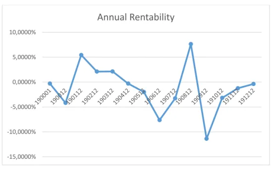
Analysing the annual index rentability it is possible to see two decline trends in the Lisbon exchange market. The first decline trend is between 1901 and 1907, where the total drop was of 13.2%. The second decline trend is between 1908 and 1910, where the total drop was of 16.2%.

The mean stock return during this period was approximately 1.18% (table 3) and the standard deviation shows us that the results during this period had a small annual variation with a standard deviation 0.049.

Table 3: Annual index Rentability

Annual Rentability

Mean 1.17919%

Standard Deviation 0.048768

Source: Own source based in information given the GHES

Figure 2: Annual Lisbon Stock Index returns

-15,0000% -10,0000% -5,0000% 0,0000% 5,0000% 10,0000%

Annual Rentability

(29)

29

Comparing the monthly with the annual rentability the conclusion is that the monthly rentability was negative and had a standard deviation less than the annual rentability. This behaviour is according theory because high rentability implies higher volatility. What concerns the monthly rentability of stock returns between 1903 and 1913 it can be explain by the number of months with negative rentability – 87 in a total of 167 observations (52%), and a number of months with a low positive rentability.

(30)

30

Chapter 6 – Results

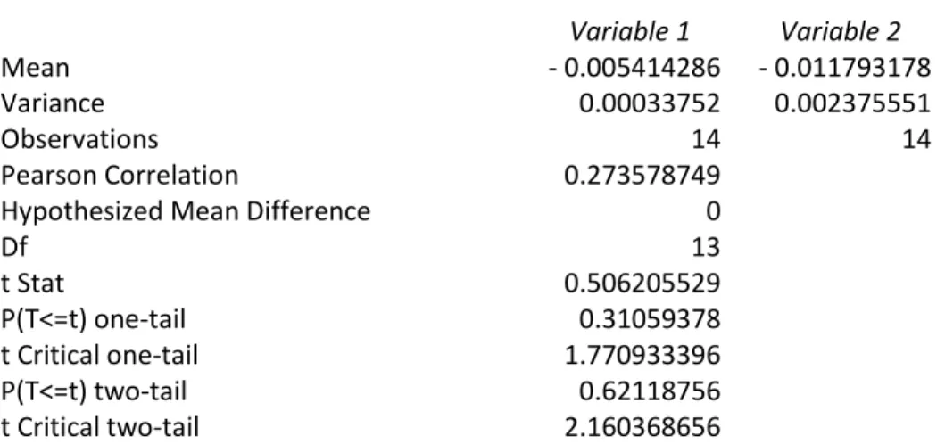
Taking into account the hypothesis described in the previous chapter and aiming to test the correlation between the different variables, in this chapter an analysis via T-test and a description of the results will be made, comparing the results obtained with the theoretical framework. The first hypothesis is rejected for the Portuguese case since there is a positive correlation between inflation and rentability of 0.2736. A possible explanation for this result is related to inflation in Portugal during this period, which the majority of the time was negative inflation. Another explanation for the Portuguese stock market to have a different correlation from the exposed in literature review is that the theory has as base the major stock markets like USA, Germany or UK and there are others specificities in these stock markets. Portugal was an emergent market with low dimension and low level of transactions (see chapter 4).

The Pearson result shows the importance of the test as there is a positive correlation between inflation and rentability of 0.2736.

Table 4: Relation between inflation and rentability

T-Test: Paired Two Sample for Means

Variable 1 Variable 2

Mean - 0.005414286 - 0.011793178

Variance 0.00033752 0.002375551

Observations 14 14

Pearson Correlation 0.273578749

Hypothesized Mean Difference 0

Df 13 t Stat 0.506205529 P(T<=t) one-tail 0.31059378 t Critical one-tail 1.770933396 P(T<=t) two-tail 0.62118756 t Critical two-tail 2.160368656

(31)

31

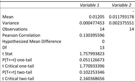
The results of the second hypothesis tested in the Portuguese stock market were aligned with the theory which stated that there was a positive correlation between nominal GDP growth and rentability of 0.1304, which shows to be a not so strong correlation. Therefore, in a period of broad increase of nominal GDP, even if 1911 had a negative performance, there is a positive correlation with stock performance.

Table 5: Relation between nominal GDP and rentability

Variable 1 Variable 2 Mean 0.01205 -0.011793178 Variance 0.000477453 0.002375551 Observations 14 14 Pearson Correlation 0.130395596

Source: Own elaboration based on information given the GHES

The results of the third hypothesis tested in the Portuguese stock market were aligned with the theory which stated that there was a negative correlation between nominal interest rate and rentability of -0.1668, which, according to these results, shows to be a not so strong correlation

(32)

32

Table 6: Relation between nominal interest rate and rentability

Mean 0.05695 - 0.011793178

Variance 0.00001 0.002375551

Observations 14 14

Pearson Correlation - 0.166781633

Testing the fourth hypothesis in the Portuguese Stock market, the results were the opposite of the ones stated in the theory, having a correlation of -0.4063. The theory stated that the relation between industrial growth (industrial GDP) and rentability was a positive relation although when analysing the Portuguese performance it is possible to see a negative relation. This result is explainable by the number of industrial companies in the General Index considered (5 out of 19).

In the beginning of the 20th century, Portugal was a peripheral country and so, it was not at the

(33)

33

Table 7: Relation between industrial growth (industrial GDP) and rentability

Mean 0.029935714 - 0.01179

Variance 0.011958646 0.002376

Observations 14 14

Pearson Correlation - 0.406265751

The results of the fifth hypothesis in the Portuguese stock market show that there is a negative correlation between real GDP variable and rentability, since the Pearson correlation has a negative result of -0.3424. This result is explainable by the impact of inflation that reduced the growth rate of GDP

(34)

34

Table 8: Relation between real industrial GDP and rentability

T-test: Paired Two Sample for Means

Mean 0.026664286 - 0.011793178

Variance 0.000370258 0.002375551

Observations 14 14

Pearson Correlation -0.342401564

Testing the sixth hypothesis, in Portuguese Stock market the results were aligned with the theory which states that there is a positive correlation between real industrial GDP variable and rentability (0.01993).This results are aligned with the theory in spite of this correlation is almost inexistent as the result is approximately zero. Probably, this result can have the same explanation of the fourth hypothesis.

(35)

35

Table 9: Relation between real industrial GDP and rentability

Mean 0.008612857 - 0.011793178

Variance 0.002361569 0.002375551

Observations 14 14

Pearson Correlation 0.019924349 Hypothesized Mean Difference 0

df 13 t Stat 1.12056136 P(T<=t) one-tail 0.141374604 t Critical one-tail 1.770933396 P(T<=t) two-tail 0.282749208 t Critical two-tail 2.160368656

The results of the seventh hypothesis imply its rejection. In the Portuguese stock market there is a positive correlation between real interest rate and rentability, since the Pearson correlation has a positive result of 0.4711. This result is the opposite of what the authors have defined as the theory states that there is a negative correlation between real interest rate and rentability.

An explanation for these results can be related with the lack of financial alternatives of investment in the Portuguese financial market. Since 1891 Portugal was in a financial crisis that strangles financial investment alternatives. Another explanation can be the lack of knowledge about the positive behavior of real interest rate.

(36)

36

Table 10: Relation between real interest rate and rentability

Mean 0.055858571 - 0.011793178

Variance 0.000381151 0.002375551

Observations 14 14

Pearson Correlation 0.47103098

The results of the eighth hypothesis, in the Portuguese economy were aligned with the theory which states that there is a negative correlation between real GDP variable and inflation variable. This correlation between real GDP and inflation in the Portuguese economy is negatively associated by 0.6402. This negative result can be explained by the simple factor that inflation is known to be a monetary effect and there is a general consensus around the policymakers as well as central banks that inflation is harmful for the real GDP growth. The same path had occurred in Portugal during the first decade of the 20th_century.

(37)

37

Table 11: Relation between Real GDP and Inflation

t-Test: Paired Two Sample for Means

Variable 1 Variable 2 Mean 1.745 - 0.541428571 Variance 8.080073077 3.375197802 Observations 14 14 Pearson Correlation - 0.64025954

df 13 t Stat 2.008508265 P(T<=t) one-tail 0.032914556 t Critical one-tail 1.770933396 P(T<=t) two-tail 0.065829112 t Critical two-tail 2.160368656

(38)

38

Chapter 7 – Conclusions

The study of Lisbon Stock Exchange as well as the macroeconomic variables, which underlies the correlation between stock return, has been an international recurring topic in order to get some clues to future trends in stock markets. In what concerns Lisbon Stock Market there are not too many studies about the correlation between stock market and macroeconomic variables and there are no studies for the period of 1903-1913.

The analysis of the macroeconomic situation in Portugal at the beginning of 20th_{century shows us}

a country with some industrialization, but when this industrialization is compared with countries like the United Kingdom or Germany there is only one possible conclusion which is that Portugal was a peripheral economy.

Comparing the Lisbon Stock Exchange with other international stock exchange, it is possible also to conclude that the weight of Lisbon Stock Exchange in the Portuguese economy was comparable to other peripheral countries. The number of securities that were transacted was very low indeed and the higher number of shares traded were from banks and large companies. The rentability between 1903 and 1913 was not also very high and during a lot of months the Lisbon Stock Exchange had a negative rentability.

Analysing the results of the different hypothesis considered some conclusions about the Lisbon Stock Market can be reached. The Lisbon Stock Market follows a peculiar trend, since from the eight hypothesis tested, only five of them had the same behaviour as expected by the authors. The hypothesis rejected were: the hypothesis of having a negative correlation between inflation and rentability; having a positive correlation between industrial growth, GDP and rentability; and having a negative correlation between real interest rate and rentability.

We can conclude that in Portugal between 1903 and 1913, real GDP and inflation had a negative correlation, but inflation and rentability had a positive correlation. This last result – inflation and rentability – was not according theory, but we had between 1903 and 1913 low inflation and low rentability. Concerning GDP (nominal and real) this variable had a positive correlation with rentability. The same cannot be conclude when the variable is the industrial GDP. The low number of industrial companies quoted in the Lisbon Stock Exchange can be an explanation for this result. If we consider interest rate, a variable very important for the choice between money and other

(39)

39

assets, the conclusion was that real interest rate had a positive effect in the rentability. The opposite with nominal interest rate that had a negative correlation with rentability, as predicted by theory. As during this period Europe was facing social and political instability, for a further academic work it would be interesting to propose a study comparing the Lisbon Stock Market performance during the period of 1903-1913 with other European stock markets in the same period, showing the differences and similarities, or a study concerning the performance of Lisbon Stock Exchange

(40)

40

References

Branco, A., Neves, P. and Sousa, R. (2015), “The dynamics of Lisbon Stock Exchange during the first era of financial globalization, 1870-1913”, paper presented in the International Workshop

Cores and Peripheries in National Capital Markets: Exploring the Role of Regional Stock Exchanges, 19th – 20th, Universidad Carlos III, Madrid.

Costa, L., Lains, P. and Munch, S. (2011), História económica de Portugal: 1143-2010, A Esfera

dos Livros.

Fama, E. (1977), Assets returns and inflation. Journal of Economics Vol. V (2), 115-146.

Fama, E. (1981), Stock returns, real activity, inflation and money. American Economic

Association, Vol. CIII (1) and CIV (8), 545-565.

Fisher, I. (1930), The theory of interest, 1st_{ed. New York: Macmillan Company.}

Flandreau, M. and Zumer, F. (2004), Les origines de la mondialisation financière 1880-1913, 1st

ed. New York: OCDE.

Gerschenkron, A. (1962), Economic backwardness in Historical Perspective, 1st ed. Cambridge:

Havard University Press.

Geske, R. and Roll, R.(1983), The fiscal and monetary linkage between stock returns and inflation,

Journal of Finance, Vol. XXXVIII (1), 1-33.

Hull, J. (2008), Options, futures and other derivates, 7th ed. New York: Prentice-Hall.

Jaffe, J. and Mandelker, G (1976). The “Fisher effect” for risky assets: An empirical investigation,

Journal of finance, Vol. XXXI (2), 447-458.

Kaul, G. (1987), Stock returns and inflation: The role of the monetary sector, Journal of Financial

Economics, Vol. XVIII (2), 253-276.

Kessel, R. (1956), Inflation caused wealth redistribution: a test of a hypothesis, American

Economic Review, Vol. XLVI (1), 128-141.

Lains, P. (1990), A evolução da agricultura e da indústria em Portugal (1850-1913): uma

interpretação quantitativa, Banco de Portugal.

Lee, B. (1992), Causal relations among stock returns, interest rates, real activity and inflation,

(41)

41

Linter, J. (1975), Inflation and security returns, Journal of Finance, Vol. XXX (2), 259-280.

Mandelker G. (1976), The “fisher effect” for risky assets: An empirical investigation, Journal of

finance, Vol XXXI (2), 447-458.

Mata, E., Valério, N. (2011), The Concise Economic History of Portugal: A Comprehensive Guide, Almedina.

McDonald, J. (2014), Handbook of biological Statistics, 1st_ed. _Baltimore: _{Sparky House}

Publishing.

Mundell, R. (1963), Inflation and real interest, Journal of Political Economy, Vol. LXXI (3), 280-283.

Nelson, C. (1976), Inflation and rates of return on common stocks, Journal of Finance, Vol. XXI

(2), 471-483.

O´Rourke, K. and Williamson, J. (1999), globalization and history, the evolution of a

nineteenthcentury Altantic Economy, 1st ed. Cambridge, Massachusetts: MIT University Press.

Rajan, R. G. e Zingales, L. (2003), «The Great reversals: the politics of financial development in the twentieth century», Journal of Financial Economics, 69, pp. 5-50.

Reis, J. (1992), O atraso Económico português 1850-1930, 1st _{ed. Lisboa: Imprensa Nacional Casa}

da Moeda.

Ulrich, E. (1906), Da Bolsa e Suas Operações, 3rd ed. Coimbra: Coimbra Impresa da Universidade.

Trebilcock, C. (1982). The industrialization of the Continental Powers 1780-1914, 1st ed.

Longman: Routledge.

Valério (coord.) (2001), Estatísticas Históricas Portugal, 1st ed. Lisboa: Gabinete de História Económica e Social

Lains, P. (1990), A evolução da agricultura e da indústria em Portugal (1850-1913): uma

interpretação quantitativa, Banco de Portugal.

Websites:

■ Guide for referencing unexpected inflation and expected inflation. Available in http://www.farlex.com [online access on: 2015/3/12]

(42)

42

Appendix

Table I: Economic development indicators

Portugal Europe

GNP per capita (dollars)

Cities with more than 5000 inhabitants Railways (kilometres by square Kilometer) Cotton consumption (kilograms per capita) Cotton spindles/1000 inhabitants

Iron consumption (kilograms per capita) Coal consumption (kilograms per capita)

290 17% 0.033 2.97 80.6 11.1 200 499 36% 0.104 5.81 237.0 80.0 1,509 Source: Reis (1992)

(43)

43

Table II: Nominal GDP growth in Percentage (1890-1913)

Year Germany Spain France Italy Norway Portugal United Kingdom 1890 2.40 - 0.56 2.45 3.93 0.56 0.97 1891 - 4.44 3.48 1.40 9.38 1.30 0.30 1.89 1892 4.06 3.18 - 2.16 4.91 2.82 2.64 - 0.50 1893 1.73 2.05 - 1.90 - 10.31 - 0.37 0.57 - 2.51 1894 0.46 - 3.68 0.92 1.53 1.25 1.99 5.67 1895 1.23 - 0.03 - 4.37 - 3.33 0.87 6.42 0.35 1896 0.02 - 4.73 5.86 4.06 1.96 3.15 5.63 1897 3.67 10.23 5.78 - 2.36 5.17 - 0.64 - 0.92 1898 6.83 11.86 4.87 12.75 5.02 1.28 7.30 1899 6.43 - 2.78 2.10 0.33 8.60 1.77 8.29 1900 0 6.65 0.72 6.72 6.71 2.85 2.51 1901 10.11 5.70 - 5.69 3.21 4.69 - 2.17 6.63 1902 0.98 - 4.00 3.04 - 4.40 - 1.26 0.62 - 3.08 1903 7.75 8.05 6.30 9.00 - 1.81 3.31 - 0.65 1904 5.47 0.10 - 2.42 - 1.34 0 1.90 1.85 1905 7.15 - 0.96 0.44 5.28 2.22 0.58 3.20 1906 4.54 0.42 7.22 6.47 7.42 1.16 1.08 1907 5.74 8.83 8.78 12.41 6.57 3.32 2.04 1908 - 1.24 - 4.75 - 3.65 - 4.50 2.69 2.77 - 1.00 1909 4.52 2.62 7.43 8.58 1.31 1.40 1.72 1910 3.22 - 3.86 2.03 - 0.81 9.04 0.64 2.04 1911 5.07 6.28 10.20 10.59 6.62 - 4.32 5.41 1912 7.19 0 9.54 4.27 9.80 3.31 1.99 1913 1.70 7.14 0.37 4.10 10.54 1.50 6.71 Source : Flandreau, Zumer (2004), p.129 (adapted)

(44)

44

Table III: Nominal public debts in Europe in millions of national currency (1890-1913) Year Germany Spain France Greece Italy Netherlands Portugal United

Kingdom 1890 9,290 6,887 30,096 738 12,640 1,089 630 684 1891 10,154 6,920 30,481 816 12,945 1,112 720 677 1892 10,748 7,176 30,612 849 13,150 1,106 704 671 1893 11,083 7,228 31,035 969 13,179 1,122 712 667 1894 11,445 7,284 31,065 1,088 13,038 1,116 706 659 1895 11,628 7,400 31,094 1,152 13,275 1,104 719 652 1896 11,808 7,977 30,235 1,190 13,414 1,111 800 645 1897 11,920 8,378 30,100 1,143 13,409 1,095 840 639 1898 11,984 10,596 29,948 1,099 13,676 1,107 794 635 1899 12,260 11,449 30,055 1,140 13,712 1,149 801 639 1900 12,388 12,769 30,097 1,207 13,921 1,145 805 704 1901 12,888 13,363 30,344 1,264 13,911 1,159 771 765 1902 13,542 13,337 30,346 1,266 13,803 1,140 647 798 1903 13,813 12,744 30,375 1,274 13,684 1,152 659 795 1904 14,329 12,638 30,460 1,219 13,919 1,133 631 797 1905 14,532 12,523 30,702 1,099 13,978 1,106 643 789 1906 15,108 12,533 30,348 979 14,361 1,145 642 779 1907 16,066 12,475 30,162 874 14,613 1,140 675 762 1908 16,629 12,390 30,375 849 14,726 1,134 665 754 1909 18,501 12,471 32,864 840 14,946 1,128 661 763 1910 19,416 10,480 32,558 792 15,157 1,122 669 733 1911 19,577 10,420 32,720 759 15,545 1,117 684 718 1912 19,605 10,350 32,881 829 15,467 1,163 687 711 1913 20,189 10,372 32,889 959 16,382 1,156 --- 706 Source : Flandreau, Zumer (2004), p.124 (adapted)

(45)

45

Table IV: Short-term nominal interest rates (%) (1890-1913)

Year Germany Belgium Spain France Greece Italy Netherlands Portugal United Kingdom 1890 4.52 3.18 4.00 3.00 6.75 5.83 2.79 5.80 4.52 1891 3.78 3.00 4.06 3.00 6.50 5.21 3.12 6.03 3.28 1892 3.20 2.69 5.43 2.70 6.50 5.25 2.70 6.00 2.51 1893 4.07 2.82 5.50 2.50 6.50 6.00 3.40 6.00 3.05 1894 3.12 3.00 5.50 2.50 6.50 5.83 2.58 6.00 2.10 1895 3.14 2.61 4.63 2.10 6.50 5.21 2.50 6.00 2.00 1896 3.66 2.84 4.78 2.00 6.50 5.25 3.03 5.71 2.48 1897 3.81 3.00 5.00 2.00 6.50 5.71 3.13 5.50 2.63 1898 4.27 3.03 5.00 2.20 6.50 5.00 2.83 5.50 3.25 1899 5.04 3.91 4.58 3.06 6.50 4.65 3.58 5.50 3.74 1900 5.33 4.09 3.69 3.21 6.50 4.62 3.61 5.50 3.94 1901 4.10 3.28 3.68 3.00 6.00 4.44 3.23 5.50 3.72 1902 3.32 3.00 4.00 3.00 6.50 4.37 3.00 5.50 3.33 1903 3.84 3.17 4.16 3.00 6.50 4.56 3.40 5.50 3.75 1904 4.22 3.00 4.50 3.00 6.50 4.75 3.23 5.50 3.30 1905 3.82 3.17 4.50 3.00 6.50 4.81 2.68 5.50 3.01 1906 5.15 3.84 4.50 3.00 6.50 4.54 4.11 5.50 4.27 1907 6.03 4.94 4.50 3.46 6.50 4.60 5.10 5.50 4.88 1908 4.76 3.57 4.50 3.04 6.00 4.62 3.38 5.99 3.00 1909 3.93 3.11 4.50 3.00 6.00 4.40 2.88 6.00 3.10 1910 4.35 4.12 4.50 3.00 6.00 4.66 4.23 6.00 3.72 1911 4.40 4.16 4.50 3.12 6.25 4.96 3.45 6.00 3.47 1912 4.95 4.41 4.50 3.38 6.50 5.48 4.00 6.00 3.78 1913 5.88 5.00 4.50 4.00 6.50 5.62 4.50 5.74 4.77 Source : Flandreau, Zumer (2004), p.134 (adapted)

(46)

46

Table V: The exchange rate (unit: Escudo) Exchange rate (1891-1913) 1 Pound

1891 4$832 1892 5$735 1893 5$600 1894 5$790 1895 5$698 1896 5$853 1897 6$575 1898 7$108 1899 6$416 1900 6$320 1901 6$382 1902 5$722 1903 5$581 1904 5$413 1905 4$793 1906 4$582 1907 4$642 1908 5$199 1909 5$185 1910 4$895 1911 4$889 1912 4$974 1913 5$235

(47)

47

Table VI: Inflation rate (1891-1913)

Year Price índex (base 1914 = 100) Inflation rate

1891 83 --- 1892 85 1.02 1893 87 1.02 1894 89 1.02 1895 84 - 5.62 1896 85 1.01 1897 92 1.08 1898 96 1.04 1899 94 - 2.08 1900 91 - 3.19 1901 90 - 1.10 1902 87 - 3.33 1903 90 1.03 1904 96 1.07 1905 95 - 1.04 1906 95 0 1907 95 0 1908 96 1.01 1909 97 1.01 1910 93 - 4.12 1911 99 1.06 1912 98 - 1.01 1913 101 1.03

(48)

48

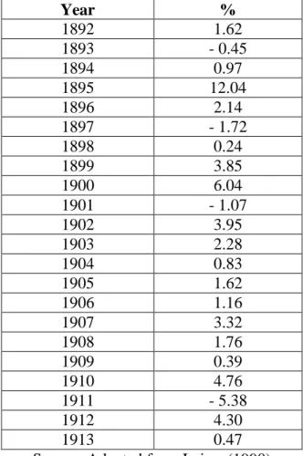
Table VII: Real interest rate (1892-1913)

Year (%) 1892 4.98 1893 4.98 1894 4.98 1895 11.62 1896 4.70 1897 4.42 1898 4.46 1899 7.58 1900 8.69 1901 6.60 1902 8.83 1903 4.47 1904 4.43 1905 6.54 1906 5.50 1907 5.50 1908 4.98 1909 4.99 1910 10.12 1911 4.94 1912 7.01 1913 4.71

(49)

49

Table VIII: Growth rate of industrial production (1890-1913)

Year % 1890 22.45 1891 - 16.27 1892 5.13 1893 11.72 1894 -13.60 1895 7.34 1896 - 12.32 1897 11.19 1898 4.76 1899 7.28 1900 11.34 1901 - 9.41 1902 5.50 1903 3.68 1904 5.40 1905 - 12.82 1906 - 4.69 1907 21.83 1908 - 7.82 1909 - 1.97 1910 21.23 1911 12.50 1912 - 6.48 1913 3.62 Source: Lains (1990)