INTRODUCTION
Bentonites are sedimentary clays formed by devitriication and subsequent chemical alteration of volcanic tuffs or ash, consisting essentially of the clay mineral montmorillonite belonging to the group of smectite. These clays are constituted by lamella formed by an octahedral sheet of alumina (Al2O3) between two tetrahedral silica sheets (SiO2). Bentonite have wide industrial applications, being used as sand binders in foundry/casting molds, in drilling luids, etc. [1-4]. Smectite clays, in addition to presenting montmorillonite clay minerals in their constitution, also
present high amounts of accessory minerals such as quartz, carbonate, mica, feldspar and kaolinite. These high levels of contaminants severely restrict their industrial applications, with the use of hydrocyclone as a likely solution for their reduction.
The hydrocyclone is important equipment for the separation of metallic and non-metallic minerals. The principle of separation is centrifugal sedimentation, in which the suspended particles are subjected to a centrifugal ield that causes their separation from the luid [5, 6]. It consists of a conical section/base connected to a cylindrical part in which there is a tangential inlet for the feed slurry.
Factorial design and statistical analysis of smectite
clay treatment by hydrocyclone
(Planejamento fatorial e análise estatística do tratamento de argilas
esmectitícas por hidrociclone)
A. J. A. Gama1, J. M. R. Figueirêdo1, A. L. F. Brito2, M. A. Gama2, G. A. Neves2, H. C. Ferreira2
1Programa de Pós-Graduação em Ciência e Engenharia de Materiais; 2CCT, UFCG,
Av. Aprígio Veloso 882, Campina Grande, PB 58429-900
[email protected], [email protected], [email protected],
[email protected], [email protected], [email protected]
Abstract
Bentonite clays are materials composed by one or more smectite clay minerals and some accessory minerals, mainly quartz, cristobalite, mica, feldspars and other clay minerals such as kaolinite. These contaminants present in clays have a large distribution of particle sizes which severely restrict their industrial applications, with the use of hydrocyclone as a likely solution for their reduction. This study aims to analyze the treatment of smectite clays from the state of Paraíba using modeling, simulation and optimization of the variable average particle diameter in relation to various process variables related to the hydrocyclone. In this study, the average diameter of smectite clays was evaluated as a function of the factors: pressure, apex diameter and vortex diameter of the hydrocyclone. Complete factorial design and addition in the central points were used to model the hydrocycloning process. The results evidenced reduction in equivalent average particle size of approximately 19.2%. Regarding the simulations, the optimum point with the lowest value was found for the average diameter of 4.033 µm, with a pressure of 4.3 bar, apex opening
of 5.3 mm, and vortex opening of 6.3 mm, all at a 95% conidence level.
Keywords: modeling, simulation, hydrocyclone, smectite.
Resumo
As argilas bentoníticas são materiais constituídos por um ou mais argilominerais esmectíticos e alguns minerais acessórios, principalmente quartzo, cristobalita, micas, feldspatos e outros argilominerais, como a caulinita. Esses contaminantes presentes nas argilas apresentam larga distribuição de tamanhos de partículas que restringem em muito suas aplicações industriais, o que aponta como provável solução para sua redução o uso do hidrociclone. Este trabalho tem como objetivo estudar o tratamento de argilas esmectitícas do estado da Paraíba utilizando modelagem, otimização e simulação da variável diâmetro médio de partículas em relação a diversas variáveis de processo relativas ao hidrociclone. Neste estudo, o diâmetro médio das argilas esmectíticas foi avaliado em função dos fatores pressão, diâmetro do apex e diâmetro do vortex do hidrociclone. Foi utilizado o planejamento fatorial completo e adição nos pontos centrais para modelar o processo de hidrociclonagem. Os resultados evidenciaram redução do tamanho médio equivalente das partículas de aproximadamente 19,2%. Em relação às simulações, o ponto ótimo de menor valor foi para o diâmetro médio de 4,033 µm para pressão de 4,3 bar, abertura do apex de 5,3 mm, abertura do vortex de 6,3 mm
para nível de coniança de 95%.
The inlet low is divided into two lows: an upper low, which leads to the overlow of the classiier and carries the lighter particles; and a lower low, which leads to the underlow of the classiier, and carries heavier particles [7, 8]. As they do not have moving parts, hydrocyclones require low investment in installation and maintenance and are simple to operate, being widely used in the chemical, mineral, textile and petrochemical industries. Some studies using hydrocyclone for the treatment of minerals have been highlighted in recent years, among them the works [9-21]. These studies concluded that this type of equipment has high eficiency in the separation of ine and coarse particles, with easy operation requiring low investment for installation and maintenance, and having relevant importance in the treatment of non-metallic minerals.
An important tool in the treatment of clays by hydrocycloning is modeling and simulation, which enables optimization of products and processes, thus minimizing duration and treatment costs, and maximizing performance, productivity and the quality of products. Modeling is able to determine and even to quantify the inluence of independent variables on treatment and on dependent variables, making it possible to obtain reliable results that can be statistically analyzed [22]. Few studies on modeling, simulation and optimization of response variables in relation to the average diameter of clay particles are found in the literature. Villasana et al. [23] studied the planning and modeling of hydrocyclone in relation to the pressure parameters and low rate of an integrated hydrocyclone system. Schneider and Neege [24] examined the hydrocyclone simulation for the treatment of non-metallic minerals. Özgenet al. [25] performed modeling and simulation with bentonite in relation to the response variables: cation exchange capacity, free swelling volume and apparent viscosity. Menezes et al. [26] evaluated the inluence of CMC (carboxymethyl cellulose) in rheological properties of smectites using simulation for use in oil well drilling luids. Boylu [12] conducted studies with sodic bentonite for optimization of hydrocyclone, and concluded that the best results were obtained with 4 bars of pressure, vortex opening of 14.3 mm, and apex of 8.0 mm.
In this study, the average diameter of smectite clays was evaluated in terms of hydrocyclone pressure factors, apex diameter and vortex diameter. A complete factorial design with addition at the central points was used to model the hydrocycloning process, as optimizing factorial design with contour surface can be successfully applied in processing clays in order to evaluate the optimum factor points, simulate the best responses, and evaluate the effects of the main factors, in addition to evaluating the interactions between the adopted factors. This study aimed to investigate the treatment of smectite clays from the state of Paraíba using modeling, simulation and optimization of the variable average particle diameter in relation to different variables related to the hydrocyclone process.
MATERIALS AND METHODS
A sample of bentonite clay from the new deposits of
the state of Paraíba, located on Campos Novos farm in the municipality of Cubati-PB, and designated as AM1 was used. The sample was enriched through disaggregation in a ball mill, then classiied through a ABNT n° 200 sieve (0.074
mm). According to [21], the chemical composition of clay was composed of: 50.77% SiO2, 21.78% Al2O3, 7.43% Fe2O3, 3.07% MgO, 2.47% CaO, 0.89% K2O, 1.30% other oxides, and 12.29% (LOI).
A RWK 42L hydrocyclone manufactured by Netzsch AWK, Germany, was used for treating this clay. It was dimensioned for particle separation with an average diameter of 2 to 5 µm. A schematic of this equipment can be found
elsewhere [27]. The process variables used in this study were: pressure (3.0 to 4.0 bar), opening of the vortex (5.0, 5.5 and 6.0 mm) and opening of the apex (3.0, 4.0 and 5.0 mm). The dispersions were prepared in the following manner: 1200 g of clay (dried in an oven at 60 °C for moisture removal)
was mixed in a volume of 30 L of distilled water with sodium hexametaphosphate at a ratio of 45.7 g/L, obtaining a dispersion of clay in water at a concentration of 4% by mass kept under agitation at a speed of 2000 rpm for a period of 24 h at room temperature. After this period, the dispersion was pumped into the hydrocyclone for centrifugation with pressures ranging from 3.0 to 4.0 bar for each coniguration of the apex and vortex.
Physical, chemical and mineralogical characterization of the sample in natura and after hydrocycloning were performed using: granulometric analysis by laser diffraction (Cilas, mod. 1064); X-ray diffraction (XRD, Shimadzu, XRD-6000), with
Kα radiation of Cu (40 kV/30 mA) and goniometer speed of
2 º/min, step width of 0.02º and scan range from 5º to 40º. Experimental planning: a bk factorial design was adopted with the addition of 3 replicates at the center point, considering the center point as the arithmetic average of the levels in the factors. In the 2k planning, k represents the number of factors and b represents the number of levels. A 23 design was used with addition of three central points, considering the factors: apex diameter, vortex diameter and pressure. Table I shows the corresponding levels of the factors. A concern in using 2k planning is the linearity assumption on the effects of factors. 2k planning works well when the linearity assumption remains approximate. Therefore, the addition of CtPt is used to increase the number of levels in 2k, meaning, from 2 to 3 levels. The central points were added in triplicate, since they do not have repercussions on estimates of the effects on planning [28, 29].
Statistical analysis of data: analysis of variance (ANOVA) was carried out in order to verify whether there are signiicant
Factor level (-1)Low point (0)Center High level (+1)
Apex diameter (mm) 3.0 4.0 5.0
Vortex diameter (mm) 5.0 5.5 6.0
Pressure (bar) 3.0 3.5 4.0
effects between the mean responses of the treatments. The procedure was used to infer whether such effects really exist, to determine the level of conidence [10]. In this case, the idea was to perform a breakdown of the variation into the variation attributed to differences between the experimental units (mean square of the residue - MSR) and the variation attributed to differences between the experimental units and attributed to the differences caused by treatments or factors (mean square of treatments - MS treat). The test is based on two hypotheses: H0: there is no main effect of factors, interaction or curvature (means are equal); Ha: there is at least one major effect of factors, interaction or curvature (means are different). The F-test was used to compare means. If the value of FCal was >FTab, the mean of the factors or interaction are different, meaning that there was effect of the factor and/or interaction. In this case, the controllable variables inluenced the response variable. If the value of FCal is ≤FTab, the means of factors or interaction are equal. This means that there is no effect of the factor and/or interaction, and that the controllable variables do not inluence the response variable. Table II shows the coniguration for Anova (analysis of variance). The coeficient of determination (R2) was calculated using Eq. A. It represents the explained variation of the model.
R2 = SQ Main -effect SQ Total
(A)
The correlation coeficient (R) was calculated using Eq. B which represents the correlation between the variables. R values range between -1 and 1, and the closer to 1 means better results. Value -1 indicates a negative linear correlation, and value 1 indicates a positive linear correlation.
R = R2 (B)
The maximum percentage of explainable variation was calculated using the Eq. C, which represents the maximum variation that the model explains. This value was compared with the value explained by the model (R2max).
R2 max = SQ Total SQ Pure_error
SQ Total (C)
In the factorial design 23 with addition of 3 CtPt (central points), the adopted model is presented in Eqs. D and E, assuming that the response surfaces are linear and/or quadratic function of factors:
y = ß0+ß1A+ß2B+ß3C+ß4AB+ß5BC+ß6ABC+ε (D)
(E)
where ß0, ß1, ß2, ß3, ß4, ß5, ß6, ß7, ß8 and ß9 are the parameter
estimates of the model, while A, B and C represent the factors adopted for apex, vortex and pressure, respectively.
RESULTS AND DISCUSSION
Fig. 1 shows the XRD patterns of the AM1sample in natura, with and without ethylene glycol. It was observed that the sample presented the following mineralogical compositions: smectite (JCPDS 29-1497), characterized by basal interplanar distances of 15.66, 3.59, 4.43 and 2.55 Å, which was conirmed by the use of ethylene glycol which increased the interlayer distance of 15.66 for 16.66 Å; presence of the kaolinite clay mineral (JCPDS 14-0164), characterized by a basal interplanar distance of 7.13 Å; presence of accessory minerals such as quartz (JCPDS 46-1045), characterized by basal interplanar distances of 4.22, 3.34, 1.82 and 1.66 Å; feldspar (JCPDS 13-0294), characterized by a basal interplanar distance of 3.22Å; and calcite (JCPDS 05-0586), characterized by a basal interplanar distance of 3.01Å. These results showed that the clay used in this study had elevated levels of accessory minerals such as kaolinite, mica, quartz, feldspar and calcite. These results are similar to preliminary results found in [19].
Fig. 2 illustrates the particle size distribution of the sample in natura. It was observed that the clay in natura presented bimodal behavior with wide distribution range varying from 0.1 to 11 µm. The clay fraction corresponded to 20.89%
(D<2 µm), D50 of 4.45µm and an average particle diameter of 5.21µm . These values were similar to those found in the
literature on bentonite clays originating in the state of Paraíba [30].
Notes: 1 - signiicant effect (F
Cal was >FTab); non-signiicant effect (FCal was ≤FTab); D.F. - degrees of freedom; R 2 -
coeficient of determination; R2max - maximum explainable variation.
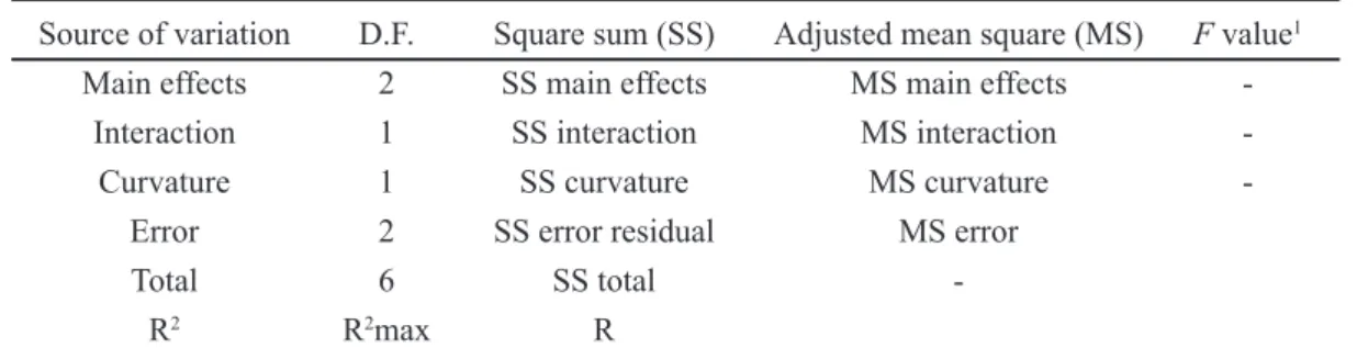
Source of variation D.F. Square sum (SS) Adjusted mean square (MS) F value1
Main effects 2 SS main effects MS main effects
-Interaction 1 SS interaction MS interaction
-Curvature 1 SS curvature MS curvature
-Error 2 SS error residual MS error
Total 6 SS total
-R2 R2max R
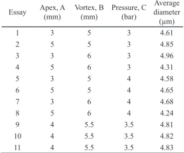
Table III contains the results of the average diameter of particle sizes. Regarding the hydrocyclone process variables, from in natura clay particle size distribution (Fig. 2), a reduction in the average equivalent diameter of the particles was found to be approximately 19.2% for the coniguration apex 5 mm, vortex 6 mm and pressure 4 bar. In general, it can be concluded that the increased pressure and apex/ vortex openings have very important inluence on the hydrocycloning process in relation to the reduction in particle size, a fact that can greatly contribute to the use of these clays for new industrial applications. In studies [21, 30] on the use of hydrocycloning for low pressures below 3 bar, it was found that the clay fraction concentrate values were lower than those 40
25 45
0 5 10 15 20 25 30 35 40 45
0 100 200 300 400 500 600 700 800 E (d=3.59A)
E (d=2.55 A) X(d=3.01 A) F(d=3.22 A) Q(d=3.34 A) Q(d=4.22 A)
E (d=4.43 A)
M(d=5.11 A) M(d=10.59 A)
C(d=7.13 A) E (d=16.66 A) E (d=15.66 A)
Whithout ethylene glycol With ethylene glycol
E - smectite M - mica C - kaolinite Q - quartz F - feldspar X - calcite
Figure 1: X-ray diffraction patterns for the AM1 sample in natura,
with and without ethylene glycol.
[Figura 1: Difratogramas de raios X para a amostra AM1 in natura com e sem etilenoglicol.]
800 400 600 200 700 300 500 100 0 0
2q (degree)
In te n s ity (a .u .)
5 10 15 20 25 30
Figure 2: Particle size distribution of the sample in natura. [Figura 2: Distribuição do tamanho de partículas da amostra in natura.]
1 10 100
0.0 0.5 1.0 1.5 2.0 2.5 3.0 3.5 4.0 4.5 0 20 40 60 80 100 D50= 4.45m
D90=10.55m DM= 5.21m <2m= 20.89m 4.5 2.5 3.5 1.5 0.5 4.0 2.0 3.0 1.0 0.0 1
Particle size (µm)
C u m u la ti v e v o lu m e (% ) In c re m e n ta l v o lu m e (% ) 100 80 60 40 20 0 100 D50=4.45 µm D90=10.55 µm DM=5.21 µm <2 µm =20.89 µm
Table III - Average diameter of particle sizes after hydrocycloning.
[Tabela III - Diâmetro médio do tamanho de partícula após hidrociclonagem.]
Essay Apex, A (mm) Vortex, B (mm) Pressure, C (bar) diameter Average (µm)
1 3 5 3 4.61
2 5 5 3 4.85
3 3 6 3 4.96
4 5 6 3 4.31
5 3 5 4 4.58
6 5 5 4 4.65
7 3 6 4 4.68
8 5 6 4 4.24
9 4 5.5 3.5 4.81
10 4 5.5 3.5 4.82
11 4 5.5 3.5 4.83
Source of variation D.F. Square sum (SS) Adjusted mean square (MS) F value
Apex 1 0.076050 0.076050 760.501
Vortex 1 0.076050 0.031250 312.501
Pressure 1 0.042050 0.042050 420.501
Apex*Vortex 1 0.245000 0.245000 2450.001
Apex*Pressure 1 0.000200 0.000200 2.002
Vortex*Pressure 1 0.001800 0.001800 18.001
Apex*Vortex*Pressure 1 0.018050 0.018050 180.501
Curvature 1 0.000200 0.096218 962.181
Error 2 0.000200 0.000200
Total 10 0.510818
R2=99.96% R2max=99.96% R=0.998
Notes: 1 - signiicant effect (F Cal≥FTab);
2 - non-signiicant effect (F
Cal<FTab); D.F. - degrees of freedom; R 2 -
coeficient of determination; R2max - maximum explainable variation.
Table IV - Analysis of variance (ANOVA) for three factors of average diameter (µm).
obtained in this study.
Table IV shows the ANOVA (analysis of variance) results of the average diameter. It was observed that all the factors were signiicant at a 95% conidence level, except for the interaction between the apex factor and pressure. By evaluating only the apex factor and the factor pressure, we can assert with a probability of 5% error that these two factors interact without inluencing the response. On the other hand, the apex, vortex and pressure factors inluenced the response when analyzed individually. Fig. 3 shows the values of the main factor effects for the average diameter. The higher response values for the average diameters of the apex, vortex and pressure occurred when the level was at the lowest value: 3 mm for apex, 5 mm for vortex, and 3.0 bar for pressure.
In Table IV, the analysis of variance showed that a second-order model can possibly be adopted, as there is curvature in the evaluated region. However, since the obtained model (Eq. A) can explain 99.96% of the data and main effects were signiicant, Eq. F can be adopted as being predictive at a 95% conidence level. In Eq. F the principal factors apex, vortex and pressure were signiicant and appear in the equation with high coeficients, being respectively: +5.450, +4.145 and +4.325. The positive sign that precedes the factors indicates the importance of the factor in hydrocyclone. Regarding the interaction, the signiicant factors inluencing the response were: -1,015 for the apex and vortex interaction, -0.820 for the vortex and pressure interaction, and +0.190 for the apex, vortex and pressure. The model explains 99.96% of the data (R2), indicating that the experimental error presented a small contribution. Fig. 4 conirms the explanation of the model in which the adjusted values as a function of the residues were in the range between +0.001 and -0.010, indicating a small margin of error.
(F)
Regarding optimization, it was possible to obtain the optimal or stationary point of the adopted factors. In this case,
the optimum point was equal to 4.24 µm (average diameter)
which was obtained when the apex factor was equal to 5 µm,
the vortex factor was equal to 6 µm, and pressure factor to
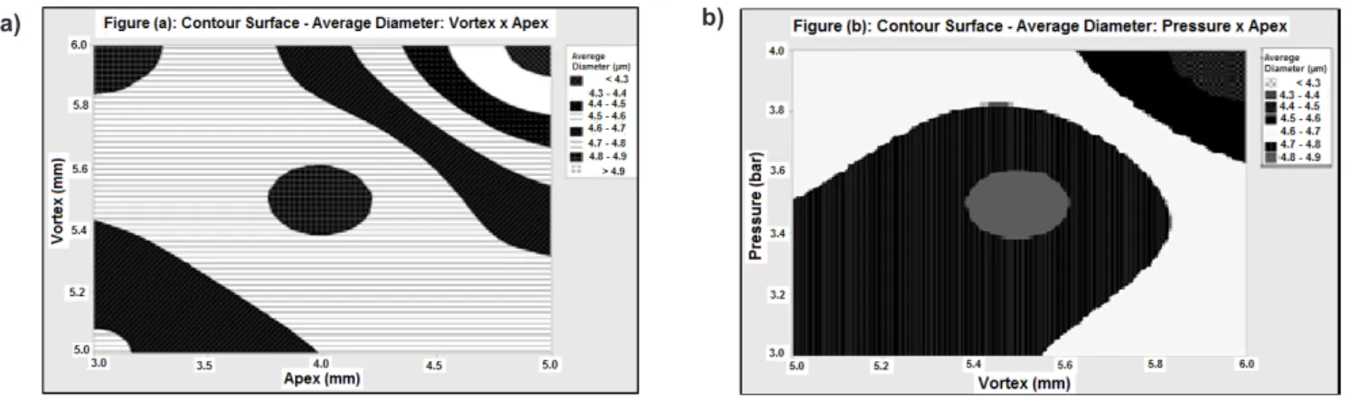
4 bar (Fig. 5). This value represents the optimal response of initially adopted factors in the experimental design. Fig. 6 illustrates the surface contour and optimized response. The interactions of the vortex and apex factors shown in Fig. 6a and the pressure and vortex interactions shown in Fig. 6b show that the best responses for the mean particle diameter are at the top of the graphs and indicate the region of the best response.From the result obtained for the optimum point (4.24 µm) which is the optimized response, several simulations in the optimum region can be performed.
Table V contains the simulated values in the optimum point region of the signiicant factors. 20 simulations were performed to test the best response of the average diameter. First, by varying the pressure and by ixing the apex and vortex (simulations 1 to 10); then, by varying all factors in the region near the optimum point (simulations 11 to 20). The lowest values for the average diameter was achieved when pressure increased. This value was obtained in the simulations 1 to 10, wherein the diameter of the apex was set at 4 mm, the vortex at 5 mm (optimal points), and the pressure in the optimum region varied (between 8 to 10.5 bar). The best result was obtained with a pressure equal to 10.5 bar, obtaining average size equal to 3.867 µm. Next, simulations Figure 3: Values of main effects for the average particle diameter.
[Figura 3: Valores dos efeitos principais para o diâmetro médio de partícula.]
Figure 4: Adjusted values x residues: average diameter.
[Figura 4: Valores ajustados x resíduos: diâmetro médio.]
Figure 5: Optimized response of apex, vortex and pressure factors.
11 to 20 were performed by varying all the factors in the regions close to the optimum point; the lowest value for the average diameter was obtained in simulation 16, wherein the value for the average diameter was equal to 4.033 µm and pressure, apex and vortex values were higher at 4.3 bar, 5.3 mm and 6.3 mm, respectively.
CONCLUSIONS
After studying hydrocyclone process variables for treating
smectite clays using modeling, simulation and optimization, it can be concluded that: i) there was a reduction in the average equivalent particle size of approximately 19.2% for the hydrocyclone coniguration of apex (5 mm), vortex (6 mm) and pressure (3.5 bar); ii) all factors were signiicant at a 95% conidence level, meaning that apex, vortex and pressure factors inluence the average diameter of the clay when analyzed individually; iii) the optimum point or minimized response was equal to 4.24 µm (average diameter) which was
obtained when the apex factor was equal to 5 mm, vortex factor was equal to 6 mm and pressure factor was 4 bar; however, by performing simulations at the optimum point, the lowest value for the average diameter equal to 4.033 µm was
found with far superior pressure, apex and vortex of 4.3 bar, 5.3 mm and 6.3 mm, respectively; iv) the process variables have a signiicant inluence in the hydrocycloning process in relation to each type of accessory minerals present in clay; a fact that can greatly contribute to the use of these clays in industrial applications.
REFERENCES
[1] P. Souza Santos, Ciência e tecnologia de argilas, 2a Ed., Edgar Blücher, S. Paulo (1992).
[2] I.A. Silva, J.M.R. Costa, R.R. Menezes, H.S. Ferreira, G.A. Neves, H.C. Ferreira, Rev. Escola Minas 66 (2013) 485.
[3] I.D.S. Pereira, V.N.F. Lisboa, I.A. Silva, J.M.R. Figueirêdo, G.A. Neves, R.R. Menezes, Mater. Sci. Forum 798-799, (2014) 50.
[4] Z. Gong, L. Liao, L. Guocheng, X. Wang, Appl. Clay Sci. 119 (2016) 294.
[5] E.A. Barbosa, L.G.M. Vieira, C.A.K. Almeida, J.J.R. Damasceno, M.A.S. Barrozo, Mater. Sci. Forum 416 (2003) 317.
[6] J.A. Sampaio, G.P. Oliveira, A.O. Silva, Rio de Janeiro, CETEM/MCT (2007) 139.
[7] O.J. Soccol, L.N. Rodrigues, T.A. Botrel, M.N. Ullmann, Braz. Arch. Biol. Technol. 50, 2 (2007) 193.
[8] D. Azizi, S.Z. Shafaei, M. Noaparast, H. Abdollahi, Trans. Nonferrous Met. Soc. China 22 (2012) 2295.
Table V - Simulated values: optimum point region (average diameter in µm).
[Tabela V - Valores de simulações: região no ponto ótimo (diâmetro médio em µm).]
Simulation factorApex Vortex factor Pressure factor value (yAdjusted s)
1 4 5 8.0 4.155 µm
2 4 5 8.5 4.097 µm
3 4 5 9.0 4.040 µm
4 4 5 9.5 3.982 µm
5 4 5 10.0 3.925 µm
6 4 5 10.1 3.913 µm
7 4 5 10.2 3.902 µm
8 4 5 10.3 3.890 µm
9 4 5 10.4 3.879 µm
10 4 5 10.5 3.867 µm
11 4.9 5.9 3.9 4.309 µm
12 4.8 5.8 3.8 4.377 µm
13 4.7 5.7 3.7 4.443 µm
14 5.1 6.1 4.1 4.169 µm
15 5.2 6.2 4.2 4.100 µm
16 5.3 6.3 4.3 4.033 µm
17 5.0 5.9 3.9 4.289 µm
18 5.0 5.8 3.8 4.341 µm
19 4.9 6.0 3.9 4.270 µm
20 4.8 6.0 3.8 4.302 µm
Figure 6: Surface contour and optimized response of: (a) vortex x apex; (b) pressure x vortex.
[Figura 6: Superfícies de contorno e resposta otimizada de: (a) vortex x apex, (b) pressão x vortex.]
[9] L.Y. Chu, W. Yu, G.J. Wang, X.T. Zhou, W.M. Chen, G.Q. Dai, Chem. Eng. Process. 43, 12 (2004) 1441.
[10] D.C. Montgomery, Design and analysis of experiments,
7th Ed., John Wiley & Sons, New York (2008) 680. [11] S.O. Motsamai, Adv. Mech. Eng. 12 (2012) 14. [12] F. Boylu, Appl. Clay Sci. 83-84 (2013) 300.
[13] M.G. Farghaly, V. Golyk, G.A. Ibrahim, M.M. Ahmed, T. Neesse, Miner. Eng. 23 (2010) 321.
[14] W.J. Oats, O. Ozdemir, A.V. Nguyen, Miner. Eng. 23 (2010) 413.
[15] K. Elsayed, C. Lacor, Chem. Eng. Sci. 65 (2010) 6048. [16] P.L. Oliveira, J.M.R. Figueirêdo, G.A. Cartaxo, G.A. Neves, H.C. Ferreira, Mater. Sci. Forum 798-799 (2014) 55. [17] V. Golyk, S. Huber, M.G. Farghaly, G. Prölss, E. Endres, T. Neesse, M.A. Hararah, Miner. Eng. 24 (2011) 98. [18] A. Davailles, E. Climent, F. Bourgeois, Sep. Purif. Technol. 92 (2012) 152.
[19] J.M.R. Figueirêdo, J.P. Araújo, I.A. Silva, J.M. Cartaxo, G.A. Neves, H.C. Ferreira, Mater. Sci. Forum 798-799 (2014) 21.
[20] F.F. Salvador, N.K. G. Silva, M.A.S. Barrozo, L.G.M. Vieira, Mater. Sci. Forum 802 (2014) 250.
[21] J.M.R. Costa, I.A. Silva, H.S. Ferreira, R.R. Menezes, G.A. Neves, H.C. Ferreira, Cerâmica 58 (2012) 419.
[22] T.S. Kumar, Y.R. Murthy, Powder Technol. 221 (2012) 387.
[23] E.J.R. Villasana, T. Dyakowsji, M.S. Lee, F.J. Dickin, R.R.A Williams, Miner. Eng. 6 (1993) 41.
[24] M. Schneider, T.H. Neege, J, Miner. Process 74 (2004) 339.
[25] S. Özgen, Y. Ahmet, A. Çalişkan, E. Sabah, Appl. Clay Sci. 46 (2009) 305.
[26] R.R. Menezes, L.N. Marques, L.A. Campos, H.C. Ferreira, L.N.L. Santana, G.A. Neves, Appl. Clay Sci. 49 (2010) 13.
[27] A.J.A. Gama, J.M.R. Figueirêdo, J.M. Cartaxo, M.A. Gama, G.A. Neves, H.C. Ferreira, Cerâmica 63, 367 (2017) 336.
[28] D.C. Montgomery, G.C. Runger, Estatística aplicada e probabilidade para engenheiros, 2a Ed., LTC Ed., S. Paulo (2003) 463.
[29] D.C. Montgomery, G.C. Runger, Estatística aplicada e probabilidade para engenheiros, 4a Ed., LTC Ed., S. Paulo (2009).
[30] I.A. Silva, F.K.A. Sousa, R.R. Menezes, G.A. Neves, L.N.L. Santana, H.C. Ferreira, Appl. Clay Sci. 95 (2014) 371.
(Rec. 02/12/2016, Rev. 10/02/2017, 27/04/2017, Ac. 27/04/2017)