DATA ENVELOPMENT ANALYSIS OF RANDOMIZED RANKS
Annibal P. Sant’Anna
Departamento de Engenharia de Produção Universidade Federal Fluminense
Niterói – RJ
E-mail: [email protected]
Received November 2001; accepted September 2002 after one revision.
Abstract
Probabilities and odds, derived from vectors of ranks, are here compared as measures of efficiency of decision-making units (DMUs). These measures are computed with the goal of providing preliminary information before starting a Data Envelopment Analysis (DEA) or the application of any other evaluation or composition of preferences methodology. Preferences, quality and productivity evaluations are usually measured with errors or subject to influence of other random disturbances. Reducing evaluations to ranks and treating the ranks as estimates of location parameters of random variables, we are able to compute the probability of each DMU being classified as the best according to the consumption of each input and the production of each output. Employing the probabilities of being the best as efficiency measures, we stretch distances between the most efficient units. We combine these partial probabilities in a global efficiency score determined in terms of proximity to the efficiency frontier.
Keywords: decision aid, randomized ranks, data envelopment analysis.
Resumo
Probabilidades e chances relativas são aqui comparadas como medidas de eficiência de unidades tomadoras de decisão (DMUs). Avaliações de preferência, qualidade e produtividade costumam ser medidas com erros e estar sujeitas à influência de outras perturbações aleatórias. Reduzir as avaliações iniciais a postos e tratar estes como estimativas de parâmetros de locação de variáveis aleatórias permite calcular as probabilidades e chances relativas de cada opção ser classificada como a de maior preferência. Esta transformação amplia as distâncias entre as DMUs mais eficientes. As probabilidades e as razões de chances relativas delas derivadas podem ser combinadas em termos de proximidade à fronteira de excelência. Aqui se apresenta evidência de que os escores de eficiência derivados das probabilidades e chances relativas são mais correlacionados com as medidas que combinam que os escores derivados dos postos ou das razões de produtividade.
1. Introduction
When we fit an efficiency frontier to observed values, not taking into consideration that random factors affect the observations, we may generate false reference patterns. For this reason, it is customary to perform some analysis of sensitivity of the optimization results to small changes in the measurements. Within the field of DEA, this is considered, for instance, by Thompson et alii (1996), Simar & Wilson (1998) and Cazals, Florens & Simar (2002). We may take into consideration this probabilistic character of the measurements by treating them as estimates for location parameters of probability distributions. This is done here, in a DEA framework, by replacing, before calculating the efficiency frontier, the observed values by the probabilities, or by the odds, of the respective units being the most efficient.
Another source of uncertainty not usually taken into account is implicit in the form of measurement of inputs and outputs. We may avoid that by starting with the simple orderings of the DMUs according to the volumes of outputs generated and the volumes of inputs consumed. The transformation into the probabilities of being the best will then perform a translation from an arithmetic to a geometric scale, reducing the distances between the DMUs ranked in the last positions and increasing the distances between the better ranked. This happens because, in general terms, anytime the rank increases one unit, the probability of being the best involves a product with one less large factor, replaced by a small factor.
The terms output and input are here employed in a wide sense, of benefits that we desire to maximize and of resources employed whose unavailability would bound the growth of those benefits. Productivity ratios, for instance, may be put in the output side and risks to the environmental in the input side. But we can accept all kinds of variables, taking any sort of values. In fact, by measuring in terms of probabilities of being the best, we evaluate all variables in the same direction, so that we are able to consider any performance variable without the need of classifying into sets of inputs or outputs.
In the next two sections, the basic model and the randomized approach are proposed. In Section 4, this approach is applied to a data set of production and costs of 15 fictitious hospitals created by Sherman (1984) and to another data set of inputs and outputs of 16 real Brazilian hydroelectric plants studied by Sant’Anna & Lins (1998). In Section 5, regression models relating the efficiency scores to the variables used in generating them are adjusted. It is verified there that, whether using uniform or normal distributions to randomize the ranks, the probability transformation, as well as the odds transformation, makes each factor to contribute with a significant effect to the aggregate efficiency score, property that does not hold if we derive efficiency directly from the vectors of ranks.
2. A Basic Model
previous measurements, ranking is automatically determined; otherwise, it is possible to derive full ranking from pairwise comparison.
To derive global efficiencies from ranks, the aggregation procedure will consist in solving the linear programming problem of DEA oriented to the minimization of input, assuming a constant arbitrary input applied in all DMUs to generate as outputs the respective ranks. This implies measuring efficiency by the ratio from the best rank attained to the best possible rank, the number of DMUs.
From this starting point, we may advance towards efficiency evaluations paying more importance to the variation of a chosen variable within a given range of values or to frontiers determined by changing the measurements of some variables. Thus, the dependence of the efficiency scores on the form of measurement may be exploited to inform about efficiency gains that production units may derive from a suitable choice of production functions.
The example below leaves clear the dependence of the relative efficiency on the form the different variables involved are measured. We analyze the data provided by Sherman (1984). This data set has the property of measuring inputs in monetary terms, so that only the numerical values relative to the outputs are responsible for the indeterminacy in the implicit production function. Sherman (1984) builds a matrix of data on 15 fictitious hospitals, whose production is measured in terms of teaching units and patients attended, the patients classified into two groups, of regular cases and of severe cases. The input is supposed to be determined by a total cost measurement. Even so, there are different forms of combining the three outputs.
Sherman (1984) data are generated in such a way that for seven of the fifteen hospitals, which will become the most efficient in his analysis, total cost is a linear combination of the number of teaching units, the number of regular patients and the number of severe patients. Thus, there is a most efficient constant contribution to final cost provided by each teaching unit, another most efficient constant contribution provided by each regular patient attended and another most efficient constant contribution provided by each severe case. But it is reasonable to believe, for instance, that there might be gains of scale and gains of iteration between different services that would make total cost grow less than proportionally as the attendance increases.
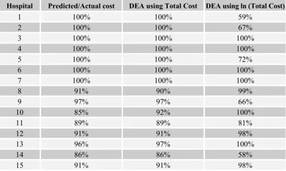
There are DEA strategies to deal with such doubt. We may, for instance, apply a logarithmic transformation to slow down costs increasing and then compare the efficiency results derived from the different approaches. Table 2.1 presents Sherman (1984) data. Table 2.2 presents the efficiencies of the 15 hospitals derived from constant returns to scale analyses assuming the input measured, respectively, by the total cost and by the logarithm of the total cost. Its first column shows the efficiency measured by the ratio between the cost predicted by the equation that fits the seven first hospitals and the observed total cost.
We can see in Table 2.2 that the first hospital, that was one of the best, becomes one of the less efficient as we transform the cost variable. Its efficiency would fall down from 100% to 59%, just 1% above that of the less efficient hospital. On the other side, the tenth hospital in the rank resulting from DEA based on Total Cost, and the less efficient if the linear model used to generate the first seven hospitals would really correspond to full efficiency, becomes one of the fully efficient.
the less preferable. Starting from that, it is easy to determine, step by step, the effects of differentiating more strongly the units with extreme values in variables such as the number of regular patients or severe cases.
Table 2.1 – Hospitals Data
Hospital Cost Teach units Regular patients Severe patients
1 775.5 50 3 2
2 816.6 50 2 3
3 841.6 100 2 3
4 800.5 100 3 2
5 950.3 50 3 3
6 1191.1 100 2 5
7 1711.3 50 10 2
8 884.8 100 3 2
9 841.6 50 2 3
10 2036.3 100 10 2
11 1362.6 50 5 3
12 1070 100 3 3
13 1491.1 50 4 5
14 898.7 50 3 2
15 1070 100 3 3
Table 2.2 – CRS Efficiency of the 15 Hospitals
Hospital Predicted/Actual cost DEA using Total Cost DEA using ln (Total Cost)
1 100% 100% 59%
2 100% 100% 67%
3 100% 100% 100%
4 100% 100% 100%
5 100% 100% 72%
6 100% 100% 100%
7 100% 100% 100%
8 91% 90% 99%
9 97% 97% 66%
10 85% 92% 100%
11 89% 89% 81%
12 91% 91% 98%
13 96% 97% 100%
14 86% 86% 58%
3. Randomized Ranks
After eliminating the uncontrolled disturbances implicit in the form of measurement, we may introduce in the analysis a controlled random component by considering the observations as location parameters of probability distributions and replacing the vectors of ranks by the vectors of probabilities of each DMU presenting the best performance according to each observed variable. The practical advantage of the transformation in probabilities of being the best is to increase the distances between the best-ranked units. This leads to efficiency frontiers simpler, in the sense of being affected by less observation units, and more informative, in the sense of making more variables affect the final result. In fact, different DMUs tend to become the best when we focus on different inputs and outputs, so that a transformation that increases the distances between the best ranked DMUs under each concept will tend to place in the frontier each variable, through a different DMU, and no more than one DMU per variable.
There are also theoretical reasons to pass from ranks to probabilities of being the best. This leads, from the linear scale of ranks, to a scale closer to the exponential scales favored in situations such as those described by Lootsma (1983), where, in the elicitation of preferences, the worst ranked options are less carefully classified. This is a reason to avoid, after replacing probabilities by odds, proceeding in the direction of logodds. Applying logarithms, besides introducing negative values, increases spaces between values near zero, what would bring us back to a more equally spaced vector of values.
The effect of substituting odds for probabilities, if all concepts are measured in the same direction, increasing from the least desirable to the most desirable observed value, is to accentuate the distances between the best-ranked DMUs. If, instead, we wish to adopt the distinction between input and output variables, probabilities may easily be adapted, by using in the position of input variable the probability of not being the unit consuming the maximum amount of resources instead of the probability of being the best. The distances between the most preferred DMUs will still be the largest. After transforming from probabilities to odds, such a natural transformation is no longer available. In fact, if we use the inverse odds to change the increasing direction of variables measuring resources consumption, the largest differences will, instead, separate the DMUs with low probabilities of being the best.
Another choice to be made is that of the probability distribution of the random disturbances supposed to affect the observations. To keep focus on observed frontiers, we should adopt, for each random variable, a probability distribution with heavy concentration around its observed values and with a light tail. On the other side, to maximize the chance of rank inversion, we must raise the probability of the values over a neighborhood wide enough to entirely cover the actually observed set. The range of such distributions should be the same for all DMUs, to mean that the random disturbances may equally affect all measurements. We suit all these principles if the distribution around each measurement is a uniform distribution centered on it and with a range large enough to allow for the possibility of change of position between any DMUs under evaluation. This determines it as the range of the observed set.
influence in the efficiency scores. But, by adding an efficient fictitious unit with the highest rank in every variable, we change substantially the results. This addition of an ideal DMU may be used to provide a pattern for comparison between the fully efficient DMUs.
The value of each input and output of each DMU is replaced by the probability or odd of such unit presenting the best possible rank with respect to the utilization of such input or production of such output. This probability is computed, following the rules above set, under the hypothesis that the measurements are independent and uniformly distributed around the respective observed values, with range equal to the difference between the largest and the smallest among the observed measurements. Formally, what we do is to replace the valuation yik of the i-th DMU under the k-th input or output by the value of P[Xik≥ Xjk, for all j ≠ i], this probability calculated following the assumption of each Xlk independently uniformly distributed on the interval [ylk – (max ymk – min ymk)/2, ylk + (max ymk – min ymk)/2]. Or by the odd, given by Oik = P[Xik≥ Xjk, for all j ≠ i]/ (1 – P[Xik≥ Xjk, for all j ≠ i]). The log-odds are the log(Oik).
To evaluate the effect of the choice of the distribution, comparisons are made in the next section not only between probabilities and odds, but also between the uniform and normal assumptions. The assumption of normality will be, as in the uniform framework above set, combined with the hypotheses of independence and identical dispersion. But, in the normal case, following the usual practice, the dispersion will be derived from the sample standard deviation instead of the sample range. The standard deviation of the Xik will still be the same for all i, but will be assumed equaling the standard deviation of the sample (y1k, …, ynk).
4. Efficiency Evaluation
The transformations above discussed are here applied to two data sets. The first was that generated by Sherman (1984), presented in Section 2. The second, studied by Sant’Anna & Lins (1998), involves, for sixteen Brazilian hydro-electric plants, three input variables, Construction Cost, Representative Fall and Maximum Volume, and one output variable, the Guaranteed Power. The first input variable globally measures the resources spent, while the other two express restrictions to production that are relaxed as their values increase.
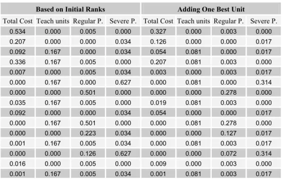
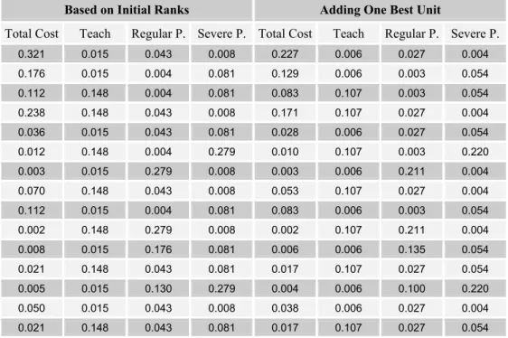
Table 4.1 presents, for the hospitals data set, the odds of being the best derived from the vectors of ranks, assuming independent uniform distributions as described in Section 3. The columns in the left side of the table present odds generated considering only the 15 original hospitals and the columns in the right side present the odds of the same hospitals becoming the best when a hospital with rank 16 is added. Table 4.2 presents the same results for the procedure with the normal assumption. Table 4.6 presents the second data set and the corresponding odds. All odds are exhibited in a 10-3 approximation.
Table 4.3 and Table 4.7 compare the DEA efficiency scores with those derived from probabilities of being the best calculated after randomization of the original values. Table 4.4 and Table 4.8 compare the efficiency scores directly derived from ranks to those obtained through the randomization of ranks.
because the ideal unit presents a best rank with respect to all variables, inputs and outputs. The distance to the frontier in terms of productivity is cumulatively affected by the increase of the distance in the two aspects.
The scores in all analyses, except those corresponding to DEA results, follow the same pattern, although a few changes in the reference units produce some order inversions. While in the hospitals data set, the efficient units are the same whether randomization is applied to ranks or to the initial values, among the hydroelectric plants, some will loose its position of fully efficient if we replace the original values by the ranks.
Examining the original data in Tables 2.1 and 4.6, we notice that ranks will overrate some small differences in the variables. This will result in some strong reductions in the probabilities of being the best and, consequently, in the efficiency scores derived from probabilities or odds. Plant 13, for instance, presents a low cost, in absolute terms that will warrant it efficiency above .9 when randomization is applied to the initial values. But, because there are 6 units with lower costs, its efficiency falls to bellow .4 when observed values are replaced by ranks before randomization. The same happens to Hospital 11 in the first data set.
Differences in the distributions of probabilities of being the best, due to ties in some input or output, will place them at different distances from the efficiency frontier. If we would consider tied, for instance, hospitals differing by only one patient, under the criteria based on the number of regular patients or the number of severe patients, or plants with differences of only 1m, under the criterion of representative fall, or only 1Mw, under the criterion of guaranteed power, we would get considerably different vectors of efficiency scores. In the hospitals data set, which presents a large number of ties, average ranks were used and probabilities equalized, while, in the hydroelectric plants data set, to accentuate this effect, a random order was used in the cases of ties.
Table 4.1 – Hospitals Uniform Odds
Based on Initial Ranks Adding One Best Unit
Total Cost Teach units Regular P. Severe P. Total Cost Teach units Regular P. Severe P.
0.534 0.000 0.005 0.000 0.327 0.000 0.003 0.000
0.207 0.000 0.000 0.034 0.126 0.000 0.000 0.017
0.092 0.167 0.000 0.034 0.054 0.081 0.000 0.017
0.336 0.167 0.005 0.000 0.207 0.081 0.003 0.000
0.007 0.000 0.005 0.034 0.003 0.000 0.003 0.017
0.000 0.167 0.000 0.627 0.000 0.081 0.000 0.314
0.000 0.000 0.501 0.000 0.000 0.000 0.278 0.000
0.035 0.167 0.005 0.000 0.019 0.081 0.003 0.000
0.092 0.000 0.000 0.034 0.054 0.000 0.000 0.017
0.000 0.167 0.501 0.000 0.000 0.081 0.278 0.000
0.000 0.000 0.223 0.034 0.000 0.000 0.127 0.017
0.001 0.167 0.005 0.034 0.000 0.081 0.003 0.017
0.000 0.000 0.126 0.627 0.000 0.000 0.072 0.314
0.016 0.000 0.005 0.000 0.009 0.000 0.003 0.000
Table 4.2 – Hospitals Normal Odds
Based on Initial Ranks Adding One Best Unit
Total Cost Teach Regular P. Severe P. Total Cost Teach Regular P. Severe P.
0.321 0.015 0.043 0.008 0.227 0.006 0.027 0.004
0.176 0.015 0.004 0.081 0.129 0.006 0.003 0.054
0.112 0.148 0.004 0.081 0.083 0.107 0.003 0.054
0.238 0.148 0.043 0.008 0.171 0.107 0.027 0.004
0.036 0.015 0.043 0.081 0.028 0.006 0.027 0.054
0.012 0.148 0.004 0.279 0.010 0.107 0.003 0.220
0.003 0.015 0.279 0.008 0.003 0.006 0.211 0.004
0.070 0.148 0.043 0.008 0.053 0.107 0.027 0.004
0.112 0.015 0.004 0.081 0.083 0.006 0.003 0.054
0.002 0.148 0.279 0.008 0.002 0.107 0.211 0.004
0.008 0.015 0.176 0.081 0.006 0.006 0.135 0.054
0.021 0.148 0.043 0.081 0.017 0.107 0.027 0.054
0.005 0.015 0.130 0.279 0.004 0.006 0.100 0.220
0.050 0.015 0.043 0.008 0.038 0.006 0.027 0.004
0.021 0.148 0.043 0.081 0.017 0.107 0.027 0.054
Table 4.3 – Hospital Scores for Randomization applied to Initial Values
HOSPITAL SCORE
DEA Uniform probability Uniform odd Normal probability Normal odd
1 1 1 1 1 1
2 1 0.81 0.76 0.94 0.9
3 1 1 1 1 1
4 1 1 1 1 1
5 1 0.31 0.26 0.64 0.58
6 1 1 1 1 1
7 1 1 1 1 1
8 0.9 1 1 1 1
9 0.97 0.69 0.64 0.87 0.83
10 0.92 1 1 1 1
11 0.89 0.05 0.03 0.29 0.21
12 0.91 1 1 1 1
13 0.97 1 1 1 1
14 0.86 0.45 0.4 0.69 0.65
Table 4.4 – Hospital Scores for Randomization applied to Ranks
HOSPITAL SCORE
Rank Uniform probability Uniform odd Normal probability Normal odd
1 1 1 1 1 1
2 1 0.58 0.44 0.92 0.81
3 1 1 1 1 1
4 1 1 1 1 1
5 0.94 0.10 0.07 0.48 0.41
6 1 1 1 1 1
7 1 1 1 1 1
8 1 1 1 1 1
9 0.95 0.33 0.22 0.73 0.62
10 1 1 1 1 1
11 1 0.60 0.48 0.86 0.79
12 1 1 1 1 1
13 1 1 1 1 1
14 0.81 0.62 0.41 0.36 0.30
15 1 1 1 1 1
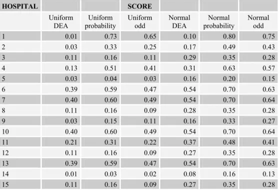
Table 4.5 – Hospital Scores with Ideal DMU Added
HOSPITAL SCORE
Uniform DEA
Uniform probability
Uniform odd
Normal DEA
Normal probability
Normal odd
1 0.01 0.73 0.65 0.10 0.80 0.75
2 0.03 0.33 0.25 0.17 0.49 0.43
3 0.11 0.16 0.11 0.29 0.35 0.28
4 0.13 0.51 0.41 0.31 0.63 0.57
5 0.03 0.04 0.03 0.16 0.20 0.15
6 0.39 0.59 0.47 0.54 0.70 0.63
7 0.40 0.60 0.49 0.54 0.70 0.64
8 0.11 0.16 0.09 0.28 0.35 0.28
9 0.03 0.15 0.11 0.16 0.33 0.27
10 0.40 0.60 0.49 0.54 0.70 0.64
11 0.21 0.31 0.22 0.37 0.48 0.41
12 0.11 0.16 0.09 0.27 0.35 0.28
13 0.39 0.59 0.47 0.54 0.70 0.63
14 0.01 0.03 0.02 0.08 0.16 0.13
Table 4.6 – Hydroelectric Plants Data
Original Values Uniform Odds Normal Odds
Cost Fall Volume Power Cost Fall Volume Power Cost Fall Volume Power 972 44 230000 414 0,000 0,131 0,000 0,458 0,003 0,129 0,002 0,300 91 27 881 16 0,013 0,309 0,080 0,000 0,038 0,227 0,095 0,002 75 35 10800 30 0,131 0,205 0,000 0,000 0,129 0,171 0,009 0,006 68 167 145 110 0,205 0,000 0,205 0,080 0,171 0,004 0,171 0,095 263 116 1150 130 0,000 0,000 0,012 0,131 0,009 0,006 0,038 0,129 1086 79 190200 344 0,000 0,001 0,000 0,309 0,002 0,013 0,003 0,227 46 75 1900 56 0,309 0,006 0,006 0,025 0,227 0,028 0,028 0,053 118 69 385 39 0,002 0,012 0,131 0,000 0,019 0,038 0,129 0,009 107 68 900 39 0,006 0,025 0,046 0,001 0,028 0,053 0,071 0,013 27 197 28 23 0,458 0,000 0,309 0,000 0,300 0,002 0,227 0,004 414 91 26500 138 0,000 0,000 0,000 0,205 0,004 0,009 0,004 0,171 321 50 8904 103 0,000 0,080 0,001 0,046 0,006 0,095 0,013 0,071 87 187 1088 51 0,025 0,000 0,025 0,002 0,053 0,003 0,053 0,019 83 53 14650 55 0,046 0,046 0,000 0,006 0,070 0,070 0,006 0,028 79 23 3642 17 0,080 0,458 0,002 0,000 0,095 0,300 0,019 0,003 135 78 7 55 0,001 0,002 0,458 0,012 0,013 0,019 0,300 0,038
Table 4.7 – Plants Scores for Randomization applied to Ranks
PLANT SCORE
Rank Uniform probability Uniform odd Normal probability Normal odd
1 1 1 1 1 1
2 1 0.98 0.85 1 0.98
3 1 0.78 0.66 0.89 0.81
4 1 0.91 0.76 1 1
5 0.97 0.41 0.31 0.63 0.54
6 0.96 0.75 0.68 0.80 0.76
7 1 0.83 0.73 1 0.93
8 0.91 0.41 0.31 0.60 0.52
9 0.93 0.22 0.16 0.48 0.39
10 1 1 1 1 1
11 0.92 0.54 0.45 0.64 0.58
12 0.97 0.33 0.25 0.54 0.46
13 0.7 0.10 0.08 0.31 0.24
14 0.95 0.26 0.19 0.54 0.43
15 1 1 1 1 1
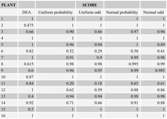
Table 4.8 – Plants Scores for Randomization applied to Initial Values
PLANT SCORE
DEA Uniform probability Uniform odd Normal probability Normal odd
1 1 1 1 1 1
2 0.475 1 1 1 1
3 0.66 0.90 0.86 0.97 0.96
4 1 1 1 1 1
5 1 0.96 0.94 1 0.89
6 0.82 0.52 0.29 0.58 0.41
7 1 0.91 0.9 0.99 0.98
8 0.615 0.98 0.98 0.995 0.99
9 0.6 0.96 0.95 0.99 0.985
10 0.87 1 1 1 1
11 0.84 0.20 0.18 0.65 0.61
12 1 0.62 0.59 0.88 0.86
13 0.4 0.94 0.94 0.98 0.98
14 0.92 0.71 0.66 0.91 0.88
15 0.5 1 1 1 1
16 1 1 1 1 1
Examining the original data in Tables 2.1 and 3.6, we notice that ranks will overrate some small differences in the variables. This will result in some strong reductions in the probabilities of being the best and, consequently, in efficiency scores derived from probabilities or odds.
If we would consider tied, for instance, hospitals differing by only one patient, under the criteria based on the number of regular patients or the number of severe patients, or plants with differences of only 1 m, under the criterion of representative fall, or only 1 Mw, under the criterion guaranteed power, we would get considerably different vectors of efficiency scores. In the hospitals data set, which presents a large number of ties, average ranks were used and probabilities equalized, while, in the hydroelectric plants data set, to accentuate this effect, a random order was used in the cases of ties.
5. Explanatory Power
It is expected that stretching the distances between the preferred DMUs and measuring efficiency in terms of proximity to the excellence frontier will result in scores representing more closely the probabilities of being the best than those derived from enveloping variables that do not emphasize excellence so strongly. An objective evaluation of such relation may be obtained through the regression of the efficiency vector on the variables entering the analysis.
relative to all explanatory variables will be small. Tables 5.1, 5.2 and 5.3 present coefficients of determination R2, F statistics and maximal p-values. Table 5.1 refers to regressions whose dependent variables are scores derived from probabilities and odds based on the ranks for the 15 hospitals data. For the measures based on the original values, the relations are similar, with a consistent reduction in the values of the goodness of fit indices.
Table 5.2 relates scores and probabilities generated by adding to the hospitals data set a fictitious hospital with a best rank of 16 with respect to every variable. The addition of this unit results in a strong improvement in all the models fit. This improvement would occur also with the original data replacing the ranks.
Table 5.3 presents the results of the adjustment of the regression of the efficiency scores of the hydroelectric plants. In this case, the models fit very well, even without the addition of the ideal unit.
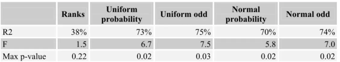
We can notice, in the three tables, that, although the vectors of efficiency scores follow the same pattern, there is a clear improvement in the regression fit as we pass from ranks to probabilities and another gain, not so strong, as we pass from probabilities to odds. After randomization is applied, all variables become significant in the determination of the efficiency scores, what did not happen for the efficiency computation based directly on the ranks.
We can also notice that the procedure based on the uniform distribution with the common range determined by the sample range, also, systematically presents better adjustment than the normal procedure.
Table 5.1 – Hospital Models Fit
Ranks Uniform
probability Uniform odd
Normal
probability Normal odd
R2 38% 73% 75% 70% 74%
F 1.5 6.7 7.5 5.8 7.0
Max p-value 0.22 0.02 0.03 0.02 0.02
Table 5.2 – Fit for Scores Resulting from Addition of Ideal Hospital
Uniform probability Uniform odd Normal probability Normal odd
R2 97% 98% 89% 92%
F 78.8 150.1 21.3 29.2
max p-value 0.02 0.02 0.02 0.02
Table 5.3 – Hydroelectric Plants Models Fit
Ranks Uniform
probability Uniform odd
Normal
probability Normal odd
R2 0.40 0.89 0.92 0.86 0.90
F 1.8 23.3 36.4 17.4 23.9
6. Conclusion
Since the distance to the efficiency frontier depends on the forms of measurement of the concepts involved, it is important to have a reference model. The models based on the ordering of the units and its probabilistic variants offer a baseline from which we may proceed to the identification of differences between DMUs associated to the form of measurement taken for each particular input or output.
Different sources of variation can be identified in the equalization of distances involved in the ranking procedure: reducing distances between effective values and artificially creating distances between effectively tied DMUs. Taking ranks as a starting point and trying to associate eventual posterior changes to the effects of these two sources constitute an effective and easy to follow strategy of searching for better transformations.
Combining the variables in terms of probabilities of being the best, and in terms of odds derived from these probabilities, by detaching more clearly the points in the frontier, helps relating the global efficiency scores to the classifications according to the particular variables. The results here obtained when the global measure of efficiency combines probabilities derived from measured values are only in special units different from those obtained when the probabilities are derived from ranks.
The evidence collected here supports the idea that odds, by stretching even more than probabilities the distances between the preferable DMUs, provide clearer explanation for the results of aggregation in terms of proximity to the excellence boundary. The use of the uniform distribution results in final scores slightly more related to the vectors of probabilities of being the best according to the particular variables isolatedly. The addition of an ideal unit, besides allowing to discriminate inside the set of fully efficient units, seems to increase the relation of the final scores to the partial classifications.
Acknowledgement
I am grateful to the referees for their careful and patient revision. Their comments helped improving the text substantially.
References
(1) Cazals, C.; Florens, J.P. & Simar, L. (2002). Nonparametric Frontier Estimation: a robust approach. Journal of Econometrics, 106, 1-25.
(2) Lootsma, F.A. (1993). Scale sensitivity in the Multiplicative AHP and SMART. Journal of Multicriteria Decision Analysis, 2, 87-110.
(3) Thompson, R.G.; Dharmapala, P.S.; Diaz, J.; Gonzales Lina, M.D. & Thrall, R.M. (1996). DEA multiplier analytic center sensitivity analysis with an illustrative application to independent oil companies. Annals of Operations Research, 66, 163-180.
(4) Sant’Anna, L.A.F.P. & Lins, M.E. (1998). Análise da Eficiência de Hidrelétricas a Fio d’água. Anais do XVIII ENEGEP, Niterói.
(5) Sherman, D. (1984). Data Envelopment Analysis as a new managerial audit methodology – test and evaluation. Auditing: a Journal of Practice and Theory, 4, 35-53.