Measuring market power from plantlevel data

FORTALEZA MARÇO 2007

Measuring Market Power

from Plant-Level Data

Measuring Market Power

from Plant-Level Data

Sérgio Aquino DeSouza

Measuring Market Power from Plant-Level Data

Sergio Aquino DeSouza†

ABSTRACT

Measuring the degree of market power has been the object of many applied studies in the industrial organization field. But, as this paper points out, identification problems arise when we estimate markups from production function regressions using data sets that do not report firm or plant-level physical quantities of output. In a differentiated product industry, the lack of such information introduces an unobserved (price) heterogeneity term. In this paper, I set up an econometric model that controls for this unobserved term and shows that failing to do so leads to spurious markup estimates.

I illustrate this result using data from Colombian plants. The results reveal that, if we do not control for (price) heterogeneity, we will find misleading evidence of firms with little or no market power.

*

I am thankful to James Tybout and Mark Roberts for useful comments and the Brazilian agencies, CAPES and FUNCAP, for financial support.

†

Author’s affiliation: Graduate Program in Economics (CAEN) and Department of Economic Theory, Universi- dade Federal do Ceará.. Address: Av. da Universidade, 2700, segundo andar, Fortaleza, Brazil.

2 I. INTRODUCTION

Measuring the degree of market power has been the object of many applied studies in the industrial organization field. But, as this paper points out, identification problems arise when we estimate markups from production function regressions using data sets that do not report firm or plant-level physical quantities of output. In a differentiated product industry, the lack of such information introduces an unobserved (price) heterogeneity term. In this paper, I set up an econometric model that controls for this unobserved term and show that failing to do so leads to spurious markup estimates. I illustrate this result using data from Colombian plants. The results reveal that, if we do not control for (price) heterogeneity, we will find misleading evidence of firms with little or no market power.

3 expenditure data are observed. Most researchers ignore this problem and uncover quantities by simply deflating revenue using an aggregate price index. For industries characterized by product differentiation this may not be a suitable procedure, since price dispersion is likely to be observed.

This paper is a natural extension to previous studies that discussed production function identification issues but emphasized different objects. Klette and Griliches (1996) argued that estimates of internal returns to scale that ignored the ratio of firm-specific price to the aggregate price index are asymptotically downward biased. Assuming monopolistic competition and a CES demand function they were able to control for price heterogeneity and to identify internal returns scale and the elasticity of substitution. Focusing on the productivity measure but using the same framework, Melitz (2000) found that (measured) productivity is spuriously pro-cyclical and also downward biased.

Building on the methodology developed by these authors, I develop an econometric model to estimate markups that controls for unobserved (price) heterogeneity and identifies a source of spurious markup estimates if price dispersion is ignored. These results, however, come at a cost: the assumption that capital is flexible. For this reason, a separate section is set aside to analyze the robustness of the model once this assumption is relaxed. All regressions are performed with data on Colombian plants drawn from selected manufacturing industries.

4 for the measurement of markups. The data and the construction of variables are described in Section IV. The estimation results are presented and discussed in section V. Further, this paper devotes a separate section (VI) to evaluate the robustness of our conclusions once the assumption of flexible capital is relaxed. Finally, the last section presents some concluding remarks.

II. HALL’S APPROACH

In this economy, gross output Q is generated with capital (X1), labor (X2), and an intermediate input (X3) adjusted by a term W that indexes the productivity levels. That is, firm i in year t has the following production function.

(1) Qit =F(X1it,Xit2,Xit3,W)

where F is homogeneous of degree γ in capital, labor and materials, and of degree one in W. Note that the assumption of linear homogeneity in W is made without loss of generality since W is just an index.

Log differentiating (1), defining the lowercases as the log of the variables defined above and dropping the time index yield

(2) dx F dw Q

X F

dq w

j

j i i

j i j

i =

∑

=

3

1

where Fjis the derivative of F with respect to factor j. It is also assumed that capital,

5 factor markets are competitive. Then, firm’s input choice problem imposes the following equality at each period t

(3) P_iF_j =w_j

µ

1

Pi,wj andµ represent respectively firm i’s output price, the price of the j-th

factor of production and the price-cost ratio (also known as markup1). Now, it is possible to derive a simple expression for the input coefficients since

(4) i_j i

j i j

Q X F

µα =

where αij is equal to ( ) ( i i) j

i

jX PQ

w and henceforth referred to as the revenue share of input j. Then, substituting (4) into (2) gives

(5) dq_i =µ

∑

This equation implies that output growth is determined by a weighted sum of the inputs growth. The weights for the inputs are given by the corresponding revenue shares adjusted by a measure of market power. Equation (5) contains the original Solow residual formulation as a particular case. Indeed, in a perfectly competitive environment (µ=1) productivity growth degenerates to a simple deterministic relation 3 3

2 2 1

1dx dx dx

dq

dw= −α −α −α .

1 _{I define markup as a synonym for price-cost ratio following most studies cited in this paper. Note,}

6 Equation (5) can be rewritten to express output growth as a function of returns to scale and a cost-share weighted bundle of the inputs growth as follows

(6) i j

j ij

i c dx dw

dq =γ

∑

The symbol γ represents the returns to scale parameter and cij is the

cost-share of input j relative to total cost calculated form firm i’s accounts. To derive the equation above note that the definition of returns to scale implies

(7) ≡

∑

∑

j j j

j j

Q X F

α µ γ

and that cost and revenue shares values are constrained by the following relation

j i i

i

j c

Q P TC

=

α (TCi represents firm’s i total cost). From this equation and (7) it is easy

to show that (5) implies (6). Obviously, it is possible to work backwards and obtain (6) from (5).

7 In order to stress the problems arising from this commonly used deflation technique to proxy physical quantities of output it is convenient to write the revenue (Ri),which is equal by definition to PiQi, in growth terms, as follows.

(8) drit −dpt =dqit +dpit −dpt

Notice that the LHS of (8) of the identity above is the deflated sales proxy. In turn, the RHS has two terms. The first one is the unobserved variable we are trying to approximate and the second term is the growth of the ratio of firm-specific prices relative to the price index.

Clearly, the deflated sales proxy works under the assumption of a homogeneous product market. In this case, the price index coincides with firms’ individual prices (i.e.dpit =dpt) and the proxy is a perfect measure of each firm’s

production level. Therefore,dr_it −dp_t =dq_it, and equation (5) or equation (6) can be

8

III- Controlling for price heterogeneity

The basic strategy to control for price heterogeneity is to impose more structure in the model in order to obtain unobservables (prices) as functions of a parametric function of observables. To do so, I assume that each firm produces a single variety i and faces the following constant-elasticity-of-substituion (CES) demand

(9)

t t

t it it

P R P P Q

σ −

⎟⎟⎠ ⎞ ⎜⎜⎝ ⎛ =

where Rt is the total revenue in the industry, Pt is an aggregate price index

and σ (σ>1) is the elasticity of substitution between any two varieties. The higher σ, the higher the degree of substitution across products. I also assume that the effect of each firm’s price has a negligible effect on the price index. Therefore, σ is the own-price demand elasticity (in absolute value) and each firm act as a monopoly over its variety. It is straightforward to show that the price-cost ratio µ is constant across firms and equal toσ/(σ −1). This formulation is intuitively appealing. As goods become more similar (σ increases) the price-cost ratio approaches the competitive outcome2.

Taking the log-difference of (9) allows us to write

(10) dq_it =−σ(dp_it −dp_t)+(dr_t −dp_t)

2 _{Although this market structure, known as monopolistic competition, strongly restricts cross-effects}

9 Combining the demand equation (10), the revenue identity (8) and the revenue-share based production function (5) gives3

(11) _{t t it}

j

j it ijt t

it dp dx dr dp dw

dr σ σ σ α µ σ σ 1 ) ( 1 1 − + − + − = −

∑

Since µ

σ

σ−1

is equal to one the equation above can be further simplified

(12) t t it j

j it ijt t

it dp dx dr dp dw

dr

σ σ σ

α + 1( − )]+ −1

=

−

∑

Suppose now we are naïvely trying to measure markups by proxying unobserved quantity with the ratio of revenue to a common aggregate price index. Then, equation (5) becomes

(13) _it

j

j it ijt t

it dp dx dw

dr − =β

∑

where β is the markup estimate4. Estimating variations of (13), several plant–level data studies have found evidence of low markups, usually close to one. For example, Klette (1999) using establishment data from the manufacturing sector in Norway finds markups ranging from 0.972 to 1.088. Although his estimates are statistically different from one, they are very close to this number. Using a large sample of Italian firms, Botasso and Sembenelli (2001) find results of the same

3 _{Up to equation (8)the strategy is very similar to the one proposed by Klette and Griliches(1996).}

However, since they are interested in the estimation of the returns to scale parameter , the markup parameter µ does not appear explicitly in their equations. The remaining derivations in this section are originally developed in this paper and are crucial to argument I am trying to put forward.

10 magnitude for the markup estimates. Below, I argue that these results may be driven by a misspecification of the regression equation5.

If all assumptions underlying (12) are true, then we know what the coefficients are measuring. For instance, the coefficient on (drt –dpt) is measuring the

inverse of the elasticity of substitution and the coefficient on

∑

j

j it ijtdx

α is the number

one which has no structural interpretation. We can then determine what the coefficients of misspecified versions of (12) are actually measuring.

Note that (13) is one misspecified variant of (12) for two reasons. First, the term (drt –dpt) is omitted from (13). Second, and most importantly,

∑

j

j it ijtdx

α

appears on the RHS of (13)-with a coefficient (β) to be estimated - while in the true data generating process (12) the coefficient on

∑

j

j it ijtdx

α is one. The latter implies

the main conclusion of this paper: the true value of β is one. This means that even if we had a consistent estimator of β in hand, it would converge in probability to one, whatever the value of the true price-cost ratio. Notice that the omission of (drt –dpt) in

(13) and the possible correlation between the inputs and productivity have no bearing on this result. These will introduce biases from the true value on usual econometric estimators of β but will not change its true value. To clarify this point, define βˆ as the OLS estimator ofβ.

5 _{These papers actually use a different specification of the production function where capital is held}

11 It follows that

∑ ∑

∑ ∑

However, under the true model (12), dr_it−dp_t is given by

it t t j j it

ijtdx dr dp dw

σ σ σ

α + 1[( − )]+ −1

∑

and not by the RHS of (13). Therefore, the probability limit of the OLS estimator can be expressed as

(14) ⎟⎟⎠ ⎞ ⎜⎜⎝ ⎛ ⎟⎟⎠ ⎞ ⎜⎜⎝ ⎛ + ⎟⎟⎠ ⎞ ⎜⎜⎝ ⎛ ⎟⎟⎠ ⎞ ⎜⎜⎝ ⎛ ₋ + =

∑

∑

∑

∑

The second term in this expression is the omitted variable bias, due to the omission of (drt –dpt) in (13). The third term, commonly called the transmission or

simultaneity bias, arises from the correlation between the controls (variable inputs)

and the productivity shock. Notice that, even if these biases were negligible, the OLS estimator would converge in probability to one and not to the price-cost ratio.

12 IV. DATA

The data set analyzed in this paper was obtained from the census of Colombian manufacturing plants, collected by the Departamento Administrativo

Nacional de Estadistica (DANE), and was organized by Roberts (1996). It covers all

plants in the manufacturing sector for the 1979-1981 period and plants with ten or more employees between 1982 and 1987. This study considers six different industries6: Food Products, Clothing and Apparel, Metal Products, Printing and Publishing, Electronic Machinery and Equipment and Transportation Equipment. It should be noted that I randomly selected the industries for this study and that I paid no attention to their idiosyncrasies. The reason being the objective of this paper is to illustrate the methodological problem of ignoring price heterogeneity rather than providing a detailed study for each industry. However, an application of the methodology developed in this paper to study a particular Colombian industry would be a natural extension of this work.

This Colombian data set does not contain direct information on physical quantities or prices; rather it reports only sales revenue and input expenditures. Input data are available for book value of capital, number of employees and book value of intermediate inputs. Intermediate inputs include material, fuel and energy which are bundled together to form a unique measure X3 entering the equations defined in the last sections. Price deflators for the input expenditures and sales revenue are taken

13 from Colombian National accounts and the capital series are constructed using the familiar perpetual inventory method. Table 1 presents some summary statistics for the industries selected for this study, namely, sales revenue (mean and standard deviation), number of plants that were active during the sample period and number of plant-year observations. Unfortunately, we do not observe plant ownership. Thus, we have to assume throughout the econometric analysis that each firm owns a single plant.

Table 1

Summary statistics for selected industries in Colombia. Period 1979-1987

Sales Revenue Number of Plants

Number of Observations Industry Mean Std. Dev.

Food Products (311) _{186.9 434.0 670 5528} Clothing and Apparel (322) _{29.9 83.9 568 4447} Metal Products (381) _{47.0 96.8 366 2978} Printing and Publishing (342) _{47.4 186.6 226 1815} Electronic Machinery (383) _{118.6 232.4 137 1145} Transportation Equipment (384) _{175.4 719.3 150 1212}

Note: Sales are in millions of millions of 1979 Colombian pesos.

V. ESTIMATION

14 Equation (14) shows thatβˆ does not converge in probability to one -its true value. Indeed, the omitted variable and the transmission biases lead to an overestimation of the true value7. This could increase the βˆ estimate and give us the false impression that (13) does not necessarily yield markup estimates that reflect little or no market power. Alternative methods to remedy this problem could be applied, e.g. IV estimators. Nonetheless, OLS results proved to be sufficient to validate the argument I am trying to put forward.

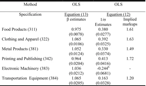
As presented in the first column of Table 2, markup estimates are close to one for all industries. Thus, even though we do not control for the sources of upward biases, the prediction that OLS estimates of markups based on (13) should be close to one still comes through. If we were to have controlled for these biases the coefficient would presumably be lower and even less plausible as markups.

The remaining task is to compare these results to the estimation of markups according to equation (12). Since input data are placed on the LHS of this equation, we do not have to worry about the simultaneity bias. Thus, simple OLS regressions can be applied without strong assumptions on the co-movements of productivity and input use. Note that a significant 1/σ estimate implies imperfect competition (σ is finite) whereas a insignificant estimate supports the alternative

7 _{Aggregate positive shocks, i.e. shocks in (dr}

t –dpt), shift out each firm’s residual demand, which in

turn raises the demand for inputs. Thus,

⎟⎟⎠ ⎞ ⎜⎜⎝

⎛

−

∑

j it

ijtdx ,dr dp

15 hypothesis of perfect competition8 .The implied markups (σ/σ-1) reported in the Table 2 show firms with high market power, considerably above one in most sectors contrasting with the previous markup estimates. This is a strong result. Controlling for price heterogeneity yields markup estimates much higher that those implied by the misspecified model (13), which already contain upward biases.

VI. Fixed Capital

It should be noted that the results developed so far are based on the assumption that capital is flexible. In this section I test whether the results obtained in the previously remain when capital is assumed to be fixed.

With fixed capital (4) does not hold for this input such that (12) is no longer valid. Obviously, the advantages of the simple econometric model discussed in the previous sections can not be claimed in this new set up. Assuming that (4) holds for the remaining inputs the log differentiated production function can be written as

(15) _i

j

i j i ij i

i dx dx dx dw

dq = +

∑

=2,3

1 1

) (

α µ γ

Specification (15) is the most commonly used in the literature. It not only relaxes the assumption of flexible capital, but also permits the simultaneous estimation of internal returns and markups. However, as shown below, neglecting price heterogeneity in this setup still leads to spurious markup estimates.

8 _{The second column of Table 2 shows estimates of 1/σ that are statistically significantly different from}

16 Equations (15), (10) and (8) form a system that yields the following equation

(16) it t t it j it j it ijt t

it dp dx dx dx dr dp dw

dr σ σ σ γ σ σ

α ( ) 1 ( 1) 1[ ] 1

3 , 2

1 = − + − + −

− −

−

∑

=

Instead of performing inference with equation (16) most researchers simply deflate revenue by a common industry price to proxy the RHS of (15), resulting in the following equation

(17) it j it j it ijtm it t

it dp dx dx dx dw

dr − = +

∑

=2,3

1 1 ) ( α λ γ

If we believe that (16) is the correct model and follow the same reasoning as in section IV it becomes clear that the true value of λ is one. Thus, any consistent estimator of λ converges in probability to one whatever the true value of the price-cost ratio. Again, the omission of (drt –dpt) and the possible correlation between

inputs and productivity have no effect on this result. They only introduce biases from the true value on usual econometric estimators of λ but do not change its true value9.

VI(i). Estimation

This section provides empirical evidence to support the main result of this paper - i.e. markup estimates, if not adjusted for price heterogeneity, are spurious – is robust to the assumption that capital is fixed. To do so, we need to estimate both the true model (16) and its misspecified version (17) and compare the results. Note that

9 _{As in the previous section, this argument is better explained when we take the plim of the OLS}

17 (16) is similar to (12). The difference is that the coefficient on capital growth (dx1)

can not be placed on the LHS of the estimating equation and, since dx1 is expected to be correlated with the error term, OLS is no longer consistent.

In the absence of good disaggregate instruments applied economists started searching for alternative methods to deal with the simultaneity problem. Levinhson and Petrin (2003)-LP hereafter- propose an econometric framework that avoids the difficult task of searching for instruments. Their method can be briefly summarized as follows. First, they assume that the intermediate input level is a deterministic function of productivity and capital. Then, by inverting this function, they are able to uncover the unobservable productivity term as a non-parametric function of the intermediate input and capital. In this way, the only unobservable error term left in the estimation is not expected to be correlated with the regressors10.

Following LP, we decompose W into two terms (W =Wo.Wu). The first term is the productivity shock observed by firms before they choose optimal labor and intermediate input levels and the second term is an i.i.d random shock11. Then, from the monotonicity property we can writeWo =Wo(X1,X3). Expressing this

function in log-differences givesdwo =dwo(x1,dx1,x3,dx3).

10

The LP framework builds on the seminal contribution of Olley and Pakes (1996). The latter authors use investment instead of intermediate input to control for the productivity term. However, the necessity to drop firms with zero-investments observations and problems that arise under a kinked investment function undermine the application of their methodology.

11 _{The first term is a state variable affecting firm’s decisions while the second term has no impact on}

18 Using a third order series approximation to this function and plugging it as a regressor in (16) yields

(18) Y_it = −1 (dx_it1)+ 1(dr_t−dp_t)+dw_ito(x1_it,dx1_it,x_it3,dx_it3)+dw_itu

σ γ

σ σ

where

∑

= −

− − ≡

3 , 2

1

) (

j

it j it ijt t

it

it dr dp dx dx

Y α . Since the observable variables

(x1,dx1,x3,dx3) control for the productivity term, 1/σ can now be consistently estimated by OLS. If we were interested in pinning down the coefficient on dx1 the LP technique becomes more involved since it is not identified in the equation above. One criticism to the LP approach is that in the same way that the intermediate input is a function of productivity so is labor. Then, in a typical production function regression where the variable inputs appear on its RHS a colinearity problem arises, casting doubt on the coefficients identification12. Nevertheless, equation (18) does not suffer from this problem as the variable inputs show up on its LHS.

Again, as shown in Table 3 the estimates are not greatly affected13 once the hypothesis of flexible capital is relaxed. The only exception is the Transportation Equipment industry14, which shows an estimate for 1/σ (0.069) well below its estimate (0.163) from equation (12). For the other sectors the implied markups are considerably above one, providing further evidence that the estimation of the misspecified production function leads to wrong conclusions about market power.

12 _{See Ackerberg et al. (2004) for a detailed discussion on colinearity problems in LP estimators.} 13 _{The Electronic Machinery industry also shows an estimate of 1/σ that is inconsistent with consumer}

behavior.

19 VII. Final Remarks

20

References

Ackerberg, D., Caves K. and Frazer, G.,2005, ‘Structural Identification of Production Functions’, Working Paper. University of Arizona.

Aitken, B. and Harrison, A.,1999, ‘Do Domestic Firms Benefit from Foreign Direct Investment? Evidence from Panel Data’, American Economic Review, 89(3), pp. 605-618.

Basu, S. and Fernald, J., 1997, ‘Returns to Scale in U.S production: Estimates and Implications’, Journal of Political Economy 105, pp. 249-283.

Botasso, A. and Sembenelli, A., 2001, ‘Market Power, Productivity and the EU Single Market Program: evidence from a panel of Italian firms’, European

Economic Review 45, pp.167-186.

Dunne, T. and Roberts, M.,1992 ‘Costs, Demand, and imperfect competition as determinants of plant-level output prices’, Discussion Paper CES 92-5, Center for Economic Studies, U.S Bureau of the Census.

Griliches, Z., 1957, ‘Specification Bias in Estimates of Production Functions’,

Journal of Farm Economics, 39, pp 8-20.

Griliches, Z. and Mairesse, J., 1995, ‘Production Functions: the Search for Identification’, NBER Working Paper No. 5067.

Hall, R., 1988, ‘The Relation Between Price and Marginal Cost in U.S. Industry’, Journal of Political Economy, 96, pp.921-947.

Hall, R., 1990, ‘Invariance Properties of Solow’s Productivity Residual’, In P. Diamond (ed.), Growth, Productivity, Unemployment, MIT Press, Cambridge, MA. Harrison, A., 1994, ‘Productivity, Imperfect Competition and Trade Reform: Theory

and Evidence’, Journal of International Economics, 36, pp. 53-73.

Klette, T.J., 1999, ‘Market Power, Scale Economies and Productivity: Estimates from a Panel of Establishment Data’, Journal of Industrial Economics, 47, pp. 451-76.

Klette, T.J. and Griliches, Z., 1996, ‘The Inconsistency of Common Scale Estimators When Output Prices Are Unobserved and Endogenous’, Journal of Applied

21 Konings, J. and Vandenbussche, H., 2004. ‘Antidumping Protection and Markups of Domestic Firms: Evidence from Firm-Level data’. LICOS Discussion Paper No.141.

Levinsohn, J., 1993, ‘Testing the Imports-as-Market-Discipline Hypothesis’, Journal of International Economics 35, pp. 1-22.

Levinsohn, J. and Petrin, A., 2003, ‘Estimating Production Functions Using Inputs to Control for Unobservables’, Review of Economic Studies, 70(2), pp. 317-342. Lindstrom, T., 1997, ‘External Economies at the Firm Level: Evidence from Swedish

Manufacturing’, Mimeo.

Melitz, M. J., 2000, ‘Estimating Firm-Level Productivity in Differentiated Product Industries’. Mimeo. Harvard University.

Mundlak, Y. and Hoch, I., 1965, ‘Consequences of alternative Specifications of Cobb-Douglas production functions’, Econometrica,33, pp. 814-828.

Olley, S. and Pakes, A., 1996, ‘The Dynamics of Productivity in the Telecommunications Equipment Industry’, Econometrica, 64(6), pp. 1263-1297. Roberts, M., 1996, ‘Colombia, 1977-85: Producer Turnover,Margins, and Trade

Exposure’, In Mark Roberts and James Tybout, editors, Industrial Evolution in

Developing countries. New York: Oxford University Press.

Roeger, W., 1995, ‘Can imperfect Competition Explain the Difference between Primal and Dual Productivity Measures? Estimates from US Manufacturing’,

Journal of Political Economy, 103(2), pp.316-330.

Tirole, J., 1988, The Theory of Industrial Organization, MIT Press, Cambridge, MA. Tybout, J., 2003, ‘Plant and Firm-level evidence on the ‘New’ Trade Theories’, in

22 Table 2: Parameters Estimates when All Factors are Flexiblea

Method OLS OLS Specification Equation (13) Equation (12)

estimates 1/σ Estimates

Implied markups Food Products (311) 0.975

(0.0078)

0.380 (0.0277)

1.61 Clothing and Apparel (322) 1.065

(0.0106)

0.392 (0.0325)

1.63 Metal Products (381) 1.052

(0.0124)

0.330 (0.0374)

1.49 Printing and Publishing (342) 0.964

(0.0204)

0.413 (0.0416)

1.72 Electronic Machinery (383) 1.036

(0.0212)

-0.244b (0.0681)

- Transportation Equipment (384) 1.065

(0.0205)

0.163 (0.0328)

1.20 Notes: a Standard errors in parenthesis.

b _{Estimate is inconsistent with consumer behavior.}

Table 3: Parameters Estimates when Capital is Fixeda

Notes: a Standard errors in parenthesis.

b _{Estimate is inconsistent with consumer behavior.}

Method LP Specification Equation (18)

1/σ Estimates Implied Markups Food Products (311) 0.417

(0.2154)

1.71 Clothing and Apparel (322) 0.434

(0.1216)

1.77 Metal Products (381) 0.208

(0.1944)

1.27 Printing and Publishing (342) 0.443

(0.0412)

1.79 Electronic Machinery (383) -0.2116

(0.3510)

- Transportation Equipment (384) 0.0699

(0.5761)

23 APPENDIX A

This appendix develops the expression for the probability limit of the OLS estimators derived from equation (17).

First, defineH_it =dr_it −dp_t,V_t =dr_t −dp_t,

' 1 1 ) ( ⎟⎟⎠ ⎞ ⎜⎜⎝ ⎛ ₋

=

∑

j it ijtm it

it dx dx dx

Z α , N as the

number of firms and T as the number of periods in the panel. Also, stack Hit, Zitand Vt as follows

]' ... ...

....

[H11 H1T HN1 HNT

H = , Z =[Z11....Z1T...ZN1...ZNT]', ]'

... ...

...

[ 1 1 N N

t V V V V

V = and ε =[dw11....dw1T...dwN1...dwNT]'.

Now, (16) and (17) can be respectively rewritten in the following convenient form

(A.1) ε

σ γ

σ

σ _{⎟ + +}

⎠ ⎞ ⎜

⎝ ⎛ −

=Z V

H 1 1 1

'

(A.2) H =Z

(

)

The OLS estimates

( )

ˆ ˆ λ

γ according to (A.2) are given by

( )

However, controlling for price heterogeneity tells us that H is given by (A.1), not by (A.2). Hence, the probability limit of

( )

'

ˆ ˆ λ

γ is equal to

⎥ ⎥ ⎦ ⎤ ⎢ ⎢ ⎣ ⎡ + + ⎟ ⎠ ⎞ ⎜ ⎝ ⎛ − − _ε σ γ σ σ _V Z Z Z Z

plim( ' ) ' 1 1 1

' 1 = ε σ γ σ

σ 1 _{lim( ' ) ' lim( ' ) '}

1

1 1 1

' Z Z Z p V Z Z Z

p − + −

24