Estimating markups from plantlevel data DeSOUZA, Sergio no

Estimating Markups From Plant-Level Data

Sergio Aquino DeSouza†

Resumo

Este artigo investiga as conseqüências de ignorar a heterogeneidade dos preços na estimação de markups com uso de microdados. Demonstra-se que, ao ignorar tal heterogeneidade, as estimativas de markups são severamente tendenciosas em direção a um, independente do nível de competição. Para demonstrar tal resultado, constrói-se um modelo econométrico sob a hipótese de competição monopolística e uma função demanda CES, em um mercado de produtos diferenciados. Este modelo leva em conta a heterogeneidade não observada dos preços e mostra-se simples de estimar, dado que mesmo o método dos Mínimos Quadrados Ordinários é válido. Usando dados de fábricas Colombianas, o modelo de produtos diferenciados revela estimativas de markups consideravelmente acima da unidade, o que rejeita a hipótese de mercados em competição perfeita.

Abstract

This paper investigates the consequences of ignoring price heterogeneity on the estimation of markups using micro-data. I show that ignoring output price heterogeneity yields markup estimates severely biased towards one regardless of competitiveness levels. To do so, I set up an econometric model that assumes monopolistic competition and a CES demand function in a differentiated product market. This model controls for unobserved price heterogeneity and is easy to estimate since OLS is applicable. Using data from Colombian plants, the differentiated product model reveals markup estimates considerably higher than one, rejecting the hypothesis of competitive markets.

Keywords: Markups, Industrial Economics, Production Function, Imperfect Competition, Microdata.

Palavras-Chave: Razão Preço-Custo, Economia Industrial, Função de Produção, Competição Imperfeita, Microdados.

JEL Classification: L11,D21,D24. Classificação da ANPEC: Área 8

*

I am thankful to James Tybout and Mark Roberts for useful comments and CAPES for financial support. †

Author’s affiliation: Curso de Pós-Graduação em Economia (CAEN), Universidade Federal do Ceará, Av. da Universidade, 2700, segundo andar, Fortaleza, Brazil.

I. INTRODUCTION

Is a certain industry competitive? If not, what is the degree of market power in this industry? Answering theses questions has always been a central concern in industrial organization. One of the most important contributions in this research subject was formulated by Hall (1988, 1990), who proposed an interesting framework where markups, returns scale and productivity can be estimated from a simple production function.

Most studies using Hall’s approach used industry level data. However, the need to study firms’ behavior (e.g, entry and exit patterns, markups and productivity) at more disaggregate levels turned necessary the use of plant-level data. The advantages of utilizing more disaggregated data are twofold. First, it avoids the aggregation bias inherently present in industry level panel data. Second, it is more consistent with the underlying theoretical models where the decision unit is a firm, not an industry. However, it poses an additional difficulty, often neglected, in the estimation of production functions that is particular to the use firm-level data: unobserved quantities. Most practitioners ignore this problem and uncover output by simply deflating revenue by an aggregate price index. For the manufacturing sector, however, this may not be a suitable assumption since for even narrowly defined industries one might expect some degree of price dispersion.

This paper shows that ignoring price heterogeneity in a differentiated good market yields price-cost ratio estimates severely biased towards one regardless of competitiveness levels and that an econometric model that embodies firm specific prices implies much higher markups.

To set up the econometric model, I add to the production function assumptions about firms and consumer behavior. In this context, this model is a natural extension to previous studies that used a similar framework but emphasized different objects. Klette and Griliches (1996) argued that simple OLS estimates of internal returns to scale that ignored the ratio of firm-specific price to the aggregate price index are asymptotically downward biased. They assumed monopolistic competition and identified the internal returns scale and the elasticity of substitution in a price adjusted revenue production function. Focusing on the productivity measure but using the same framework, Melitz (2000) finds that the productivity index is also downward biased and spuriously procyclical.

Building on this methodology – defined as KGM from now on- I develop a technique for estimating markups that assumes monopolistic competition and a CES demand function in a differentiated product market. This model controls for unobserved price heterogeneity and is easy to estimate since OLS is applicable. These nice features, however, comes at a cost: strong assumptions on the firm’s decision model. For this reason a separate section is set aside to analyze the robustness of the

conclusions once these assumptions are relaxed, at least for the capital input. All regressions are performed with data on Colombian plants at the three-digit level classification according to ISIC from the period of 1979 to 1987.

This paper is organized as follows. In the next section, a simple model that highlights the consequences of omitting output price variation is derived. Section III describes the data and the construction of variables. The estimation results are presented and discussed in section IV. Further, this paper devotes a separate segment- section V- to evaluate the sensitivity of our conclusions once the strong assumption on the input decision process is relaxed. And finally, the last section presents some concluding remarks.

II. MODEL

I begin by assuming monopolistic competition in industry j where firm i

faces a demand function given by

(1)

t t t it it

P R P P Q

σ

−

⎟⎟ ⎠ ⎞ ⎜⎜ ⎝ ⎛ =

Where Rt is the total revenue of industry j, Pt is an aggregate price index and σ (σ>1) is the demand elasticity, which is also the elasticity of substitution. It is straightforward to show that the markup is constant across firms and equal to

) 1 /(σ −

σ . This formulation is intuitively appealing. As goods become more substitutable (σ goes to infinity) the markup approaches the competitive outcome.

In this economy gross output Qit is generated with capital X1, labor X2 and materials X3 adjusted by a term W that indexes the productivity levels and a random error N.

Therefore, after definingXit ≡(Xit1,Xit2,Xit3)≡(Kit,Lit,Mit)

r

, the following production function can be written as

(2) Q_it =F(Xr_it,W_it,N_it)

Where F is homogeneous of degree γ in capital, labor and materials, and of degree one in W and N. Note that the assumption of linear homogeneity in W is made without loss of generality since this is just an index.

Log differentiating (2), defining the lowercases as the log of the variables defined above and dropping the time index yield

(3) dx F dw F dN

Q X F

dq w N

j i i

j i j j

i =

∑

It’s also assumed that firms dynamic optimization problem can be well approximated by successive and independent static decision problems and that factor markets are competitive. Then, with the demand equation (1) firm’s input choice problem imposes the following equality at each period t

(4) P_i − F_j =r_ij

σ σ 1

Pi,rj, and Fjrepresent respectively firm i’s output price, the price of the

j-th factor of production and the derivative of F with respect to this factor.

Now, it is possible to derive the simple expression for the inputs coefficients since

(5) _ij

i j i j

Q X F

µα =

Where µ is the markup and αij is the revenue share of input j. Substituting (5) into (3) yields

(6) i i

j ij

i dx dw dn

dq =µ

∑

This equation, first derived by Hall (1988) implies that the output elasticity with respect to the j-th input is just this input’s revenue share adjusted by a measure of firms’ market power. It contains the Solow residual formulation as a particular case. Indeed, in a competitive environment the Total Factor Productivity reduces to a simple deterministic relation dw+dn=dq−α₁dx1 −α₂dx2 −α₃dx3.

Equation (6) can be rewritten to express output growth as a function of returns to scale and a cost-share weighted bundle of input growth (Hall,1990) as follows

(7) _{i i}

j j ij

i c dx dw dn

dq =γ

∑

The symbols γ and c represent returns to scale and cost share respectively. To derive the equation above note that the definition of returns to scale implies

(8) =

∑

∑

j j j

j j

Q X F

α µ γ

and that cost and revenue shares values are constrained by the following relation

j i i

i

j c

Q P TC =

α (TCi represents firm’s i total cost). From this equation and (8) it easy to

show that (6) implies (7). Obviously, it is possible to work backwards and obtain (7) from (6).

Hall’s formulation - equations (6) and (7) - became a widely used technique. It allowed researchers, using data sets at various aggregation levels, to obtain output elasticities, returns to scale, productivity indexes, as well as a measure of market power (µ) from simple production function estimations. However, in most data sets, firms report revenue, not absolute quantities nor prices. A usual way to proxy output is to divide firms’ revenues by an aggregate price index, common to all firms.

This approach is justified by the assumption of a homogeneous product market. In this case, the price index coincides with firms’ individual prices and the proxy is a perfect measure of each firm production level. However, ignoring fluctuations of firm-specific prices relative to the price index in a differentiated product industry can yield severe econometric problems as mentioned in the introduction. In this way, I shall develop a model that takes this potential distortion into account.

Controlling for unobserved output

Taking the log-difference of (1) and rearranging the revenue identity

(Rit=Pit.Qit) allow us to write

(9) dq_it =−σ(dp_it −dp_t)+(dr_t −dp_t)

(10) drit −dpt =dqit +dpit −dpt

The KGM methodology controls for unobserved output by combining the demand equation (9), the revenue identity (10) and the cost-share based production function (7), yielding

(11) 1 1( _{t t}) 1( _{it it})

j

j it ijt t

it dp c dx dr dp dw dn

dr − = −

∑

σ σ σ

γ σ σ

This equation illustrates the importance of controlling for unobserved prices for the estimation of returns to scale γ and productivity dw. It introduces the elasticity of substitution parameter σ and therefore a markup (µ=σ/(σ-1)) measure in the model. Thus, if firms have some market power (µ>1) and produce heterogeneous goods, γ and dw will be downward biased.

Departing from this framework, I shall demonstrate that using the revenue share in lieu of the cost share production function (7) yields an interesting equation that circumvents some of the problems in estimating (11) and identifies a source of bias in the markup estimation.

Indeed, combining (6), instead of (7), with (9) and (10) results in

(12) 1 1 ( t t) 1( it it)

j it ijt t

it dp dx dr dp dw dn

dr − = −

∑

σ σ σ

α µ σ σ

Note that the parameter on the input bundle cancels out, such that:

(13) 1[( _{t t})] 1( _{it it})

j

j it ijt t

it dp dx dr dp dw dn

dr − −

∑

µ σ

α

The estimation of (13) has several advantages over the KGM method -equation (11). First, since the factor inputs variables appear on the LHS we do not have to worry about their potential correlation with the productivity term. Therefore, even the OLS estimator is consistent. This avoids the notoriously difficult task of searching for good instruments in micro data studies. The equation above also contains the Solow residual as a particular case. If the market is in perfect competition, i.e the coefficient on (drt –dpt) is zero, equation (13) is just the computation rule for the Solow residual.

Roeger (1995) also develops a strategy to estimate1 production function parameters that avoids instrumentation and that controls for unobserved nominal prices. However, his methodology only works under the hypothesis of constant

1

See Konings and Vandenbussche(2004) for a firm level application of Roegers’s methodology.

returns to scale. Omitting variations in this parameter can cause an upward (downward) bias in the markup estimate if returns to scale are decreasing (increasing) as shown by Basu and Fernald (1997).

Ignoring price heterogeneity

Suppose we are trying to measure markups by proxying unobserved output with the ratio of output revenue to a common aggregate price index. Then, equation (6) becomes

(14) _{it it}

j

j it ijt t

it dp dx dw dn

dr − =µ

∑

Estimating variations of (14), several plant–level data studies have supported markets with low markups, usually close to one. For example, Klette (1999) using establishment data from the manufacturing sector in Norway finds markups ranging from 0.972 to 1.088. Although his estimates are statistically different from one, they are incredibly close to this number. Using a large sample of Italian firms, Botasso and Sembenelli (2001) find results of the same order of magnitude for the markup estimates. Below, I argue that these results are driven by a misspecification of the production function2.

Indeed, if we believe that (13) is the true data generating process, those estimates are not so surprising at all. By comparing (13) to (14) and defining µ) as a consistent estimator of µ as it appears in (14) it easy to show that plim µ)=1. That is, the markup measure should be one regardless of competitive levels, or at least evolve around one after considering different sources of biases from standard econometric techniques.

III. DATA

The data set analyzed in this paper was obtained from the census of Colombian manufacturing plants, collected by the Departamento Administrativo Nacional de Estadistica (DANE), and was cleaned by Roberts (1996). It covers all plants in the manufacturing sector for the 1979-1981 period and plants with ten or more employees between 1982 and 1987. This study considers six different sectors at the three digit level: 311 (Food Products), 322 (Clothing and Apparel), 381 (Metal Products), 342 (Printing and Publishing), 383 (Electronic Machinery and Equipment) and 384 (Transportation Equipment). It should be noted that I randomly selected these industries for this study and that I paid no attention to the idiosyncrasies of neither of them. This is justified here on the basis that the objective in this paper is to

2

These papers actually use a different representation of the production function where capital is held fixed. However, specification (14) serves as a better introduction to the problem caused by the omission of price heterogeneity. In later section, I shall argue that similar arguments arise once fixed capital is assumed.

illustrate the methodological problems of ignoring price heterogeneity rather than providing a detailed study for each industry. However, an application of this methodology to study a particular industry in the Colombia manufacturing sector would be a natural extension of this work.

Input data are available for book value of capital, number of employees and book value of intermediate inputs. Intermediate inputs include material, fuel and energy that are bundled together to form a unique measure M entering the equations defined in the last section. The value of gross output is also reported. Price deflators for the inputs and aggregate output are taken form Colombian National accounts and the capital data are constructed with the usual perpetual inventory method.

IV. ESTIMATION

This section presents the markup estimates according to the misspecified model (14) and the true model (13) for selected 3-digit industries in the Colombian manufacturing sector. The strategy in this section consists of estimating both models through OLS and verifying the claim that ignoring price heterogeneity by deflating output with an aggregate price index yields markup estimates whose asymptotic value should be one regardless of competition levels.

One problem arises in this strategy. OLS estimation of (14) does not yield consistent estimators of the true value of µ (µ0=1) in (14) due to the positive correlation between input choices and productivity. It is a standard exercise to show that OLS result in the overestimation of the relevant parameter. Alternative methods to remedy this problem could be applied, e.g IV and the Olley an Pakes (1996) estimators. Nonetheless, OLS results proved to be sufficient to validate the argument I am trying to put forward.

As presented in the first column of Table 1 the magnitudes of the markups are close to one although statistically different from unity for all industries except for 342. Thus, even though we do not control for the sources of upward biases, the basic prediction that OLS estimates of the markup estimates based on (14) should be close to one still comes through. If we were to have controlled for these biases the coefficient would presumably be lower and even less plausible as markups.

The remaining task is to compare these results with the estimation of markups according to the assumed true model, represented here by equation (13). Since the input data are placed on the LHS of equation (13), I do not have to worry about the simultaneity bias. Thus simple OLS regressions can beapplied without strong assumptions on the co-movements of productivity and input use. Note that a significant 1/σ estimate implies imperfect competition (σ is finite) whereas a insignificant estimate supports the alternative hypothesis of perfect competition .The implied markups (σ/σ-1) reported in the Table 1 show firms with high market power, considerably above one in most sectors contrasting with the previous markup estimates that are close to one. This is a strong result. Controlling for price

heterogeneity yields markups much higher that those implied by the misspecified model, which already contains an upward bias.

V. Fixed Capital

Although the econometric model represented by (13) is informative with respect to consistent estimation of markups, it relies heavily on the assumption that firms choose their inputs levels in a sequence of static problems and that factor markets are competitive. These assumptions are certainly more problematic for capital. In order to decide how much to invest in a given period, agents take into account past levels of capital. Indeed, dynamic models of firm’s decisions problems have emphasized capital as a state variable, which enters as a parameter in the choice of investment, employment, and materials levels.

Hence, these assumptions, crucial to derive (13), may be leading us to wrong conclusions about markups. Yet, as I shall argue below, the basic predictions of last section remain and the data also supports the same claims as before when weaker assumptions on the capital input decision are taken into consideration.

Model

Now, I assume that capital is fixed in the short-run. Thus, (5) does not hold for this input such that (13) is no longer valid. Obviously, the advantages of the simple econometric model discussed in the previous sections cannot be claimed in this new set up.

With fixed capital and assuming that (5) holds for the remaining inputs the log differentiated production function can be written as

(15) _{i i}

j

i j i ij i

i dx dx dx dw dn

dq = +

∑

=2,3

1 1

) (

α µ γ

Specification (15) is the most commonly used in the literature. Not only it relaxes the strong assumptions on capital but it also permits the simultaneous estimation of internal returns and markups. However, neglecting price heterogeneity still leads to spurious estimates of markups.

Equation (15), (9) and (10) form a system that yields the following revenue production function

(16) _{it t t it it}

j

it j it ijt t

it dp dx dx dx dr dp dw dn

dr − −

∑

= σ µ

γ σ σ

α ( ) 1 ( 1) 1[ ] 1

3 , 2

1

Instead of performing inference with equation (16) most researchers simply deflate output revenue by a common industry price, resulting in the following equation

(17) dr_it −dp_t =γdx_it1 +µ

∑

Again, if we believe that (16) is the true model it becomes clear that µ),

now the estimator of µ as it appears in (17), converges in probability to one regardless of competition levels. Note that (16) is similar to (13). The difference is the coefficient on capital (dx1) which cannot be placed on the LHS of the estimating equation and, since dx1 is expected to be correlated with the error term, OLS is no longer consistent.

In the absence of good disaggregate instruments researchers started searching for alternative methods to deal with the simultaneity problem. Leading this recent literature, the Olley and Pakes (1996) method – OP henceforth- proposes an innovative technique that avoids the difficult task of searching for instruments. This method can be briefly summarized as follows. Using the information that investment levels are a deterministic function of productivity levels and by inverting this relationship, it is possible to uncover the unobservable productivity term as a non-parametric function of investment and the state variable capital. In this way, the only unobservable error term left in the estimation is not expected to be correlated with the regressors.

Another way to deal with this problem was developed by Levinhson and Petrin (2000)-LP hereafter. They argue that investment may only respond to the “non-forecastable” part of the productivity term since the capital input may have already adjusted to its “forecastable” part. Therefore some correlation would still remain between the regressors and the error term.

By using intermediate inputs to proxy the productivity term they are able to develop a simpler methodology that improves on the OP methodology since intermediate inputs respond to the whole productivity shock. It also avoids a major drawback of the OP method, which is the necessity to drop information on industries that report zero investment in a given period.

The availability of intermediate input in our data set and the arguments discussed above make LP our natural choice for estimating equation (16). It is worth pointing out however two limitations concerning the LP method. First, it does not control for the selection bias. That is, unlike OP, it does not use information on firms shut down decision rule in the estimation process. Second, it assumes competitive and homogeneous product markets to validate the intermediate output as proxy for the unobservable term.

While the effects of former limitation can be partially attenuated by the use of the full-sample instead of a balanced panel, the effects of the latter requires a more careful look into the technique itself, for our model assumes a differentiated product market.

The basic result that supports LP is the monotonic relation between productivity and the optimal intermediate input level. In a competitive framework it is straightforward to prove that. With fixed output and input prices an increase in productivity implies a higher intermediate input marginal product at the existing input levels. Therefore, firms will decide to expand production so that marginal product reduces to equal the intermediate input price. Therefore as output goes up demand for inputs also increases.

In an oligopolistic market this monotonic property may not hold. The marginal product still follows the same qualitative movements as before, but now firms realize that prices decrease as output goes up. Thus, the net effect of a supply expansion will ultimately depend on the elasticity of demand. It is possible to set up a scenario where one firm facing higher demand elasticity actually reduces output whereas another firm facing less responsive prices increases production levels. In a monopolistic competitive environment, however, the proof of the monotonic condition is very similar to the one presented in Levinsohn and Petrin (2000) and, therefore, will be omitted here.

From the monotonic property we can write wit =w(X1,X3). Expressing this equality in differences and dropping the firm specific and time subscripts yields

dw=dw(x1,dx1,x3,dx3). Following OP (1996) a third order series approximation to this function is used. Plugging it as a regressor in (16) implies

(18) Y_it = −1 (dx1_it)+ 1[dr_t −dp_t]+dw_it(x_it1,dx1_it,x_it3,dx_it3)+dn_it

σ γ

σ σ

Where = − −

∑

j

it j it ijt t

it

it dr dp dx dx

Y α ( 1). Since the observable variables

x1,dx1,x3,dx3 control for the productivity term, 1/σ can be consistently estimated by OLS. If we were interested in pinning down the coefficient on dx1 the LP technique becomes more involved since it is not identified in the equation above.

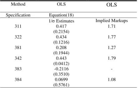
Again, as shown in Table 2 the estimates are not greatly affected once the hypothesis of flexible capital is relaxed. The only exception is the 384 sector3, which shows 1/σ estimate (0.069) contrasting with the OLS estimate (0.163) of equation (13). For the other sectors the implied markups are considerably above one, providing further evidence that the estimation of the misspecified production function yields misleading assessments about competition levels.

VI. Final Remarks

This paper shows that neglecting output price heterogeneity in plant or firm level studies can be misleading, yielding spurious markup estimates. Assuming a differentiated product market, a competitive factor market and flexible inputs yields an econometric model that demonstrates that a misspecified version of Hall’s equation implies markups equal to one regardless of the market environment. Furthermore, this model avoids the search for reliable disaggregated instruments, usually difficult to find, and can be consistently estimated by OLS. These consistent estimates, in turn, show markups much higher than one.

In a separate section, I recognize that these results are derived under restrictive assumptions on the model. Yet, relaxing the most disputable assumption imposed in the first part of the paper (flexible capital) does not change the basic result of this paper that the simple deflation of revenue by an aggregate price index without an adjustment for price heterogeneity yields misleading measurements of market power.

The framework developed here is restrictive in at least one dimension. The monopolistic competition may not be a reasonable model for many industries. It assumes that firms are not big enough to influence the aggregate market variables and therefore a price change by one firm has an irrelevant effect on the demand of any other firm. This assumption says that each product has no neighbor in the product space, which strongly restricts cross-effects and strategic interaction between products (Tirole, 1988). The discrete-choice based demand function with oligopolistic competition relaxes some of the undesirable results of the monopolistic setup. Consumers choose among N products given the product’s prices and characteristics. Producers, in turn, set optimal prices in a Bertrand fashion. This allows for a richer model of cross-effects patterns and interactions among firms. Berry, Levinsohn and Pakes (1996) develop an econometric methodology to estimate such model using market level data on prices and quantities. Along the same lines, but dealing with a data set that reports only revenue and total costs, Katayma, Lu and Tybout (2003) use a nested logit model to uncover firm-specific prices, marginal costs and other measures of firm behavior. This is certainly the path to be followed by those looking for more interactive market setups. Therefore, this paper’s message about spurious markup estimates should be taken with caution since it limits itself to raise a red flag

3

More information on this sector would be necessary to interpret this result.

for practitioners who are willing to measure markups with limited data under the monopolistic competitive market assumption.

References

Aitken, B. and Harrison, A. (1999), “Do Domestic Firms Benefit from Foreign Direct Investment? Evidence from Panel Data” American Economic Review, 89(3), pp. 605-618.

Basu, S. and Fernald, J. (1997). “Returns to Scale in U.S production: Estimates and Implications” Journal of Political Economy 105, pp. 249-283.

Bartelsman, J., Caballero, R. (1991), “ Short and Long Run externalities”, NBER Working Paper No. 3810.

Botasso, A. and Sembenelli, A. (2001) “Market Power, Productivity and the EU Single Market Program: evidence from a panel of Italian firms”. European

Economic Review 45, pp.167-186.

Caballero, R. and Lyons, R. .(1991). “Internal Versus External Economies in European Industry.” European Economic Review 34,805-26.

Cooper, R. and Johri, A. (1997) “Dynamic Complementarities: A Quantitative Analysis” Journal of Monetary Economics 40, pp. 97-119.

Griliches, Z. (1957), “ Specification Bias in Estimates of Production Functions”,

Journal of Farm Economics, 39, pp 8-20.

Griliches, Z. and Mairesse, J. (1995) “Production Functions: the Search for Identification”, NBER Working Paper No. 5067.

Hall, R.(1988). “The Relation Between Price and Marginal Cost in U.S. Industry” Journal of Political Economy 96.

Hall, R. (1990). “ Invariance Properties of Solow’s Productivity Residual”, In P. Diamond (ed.), Growth, Productivity, Unemployment, MIT Press, Cambridge, MA.

Harrison, A. (1994) “Productivity, Imperfect Competition and Trade Reform: Theory and Evidence”. Journal of International Economics 36, 53-73.

Klette, T.J. (1999): “Market Power, Scale Economies and Productivity: Estimates from a Panel of Establishment Data” Journal of Industrial Economics, 47, pp. 451-76.

Klette, T. and Griliches, Z. (1996), “The Inconsistency of Common Scale Estimators When Output Prices Are Unobserved and Endogenous,” Journal of Applied

Econometrics, 11(4), pp. 343-61.

Krizan, C. J.(1995). “External Economies of Scale In Chile, Mexico and Morrocco: Evidence from Plant-level Data”. Georgetown University, Washington, D.C.

Konings and Vandenbussche(2004). “Antidumping Protection and Markups of Domestic firms: Evidence from Firm-Level data”. LICOS Discussion Paper No.141.

Levinsohn, J.(1993). “Testing the Imports-as-Market-Discipline Hypothesis”. Journal of International Economics 35, pp. 1-22.

Levinsohn, J. and Petrin, A. (2003), “Estimating Production Functions Using Inputs to Control for Unobservables” Review of Economic Studies, 70(2), pp. 317-342.

Lindstrom, T. (1997).“External Economies at the Firm Level: Evidence from Swedish Manufacturing” Mimeo.

Lucas, R. (1988) “ On the mechanics of economic development”. Journal of

Monetary Economics, 22, pp. 3-42.

Melitz M. J.(2000) “Estimating Firm-Level Productivity in Differentiated Product Industries”. Mimeo. Harvard University.

Mundlak, Y. and Hoch, I. (1965) “ Consequances of alternative Specifications of Cobb-Douglas production functions”, Econometrica,33, pp. 814-828.

Olley, S. and Pakes, A. (1996), “The Dynamics of Productivity in the Telecommunications Equipment Industry,” Econometrica, 64(6), pp. 1263-1297.

Roberts, Mark (1996). “Colombia, 1977-85: Producer Turnover,Margins, and Trade Exposure”. In Mark Roberts and James Tybout, editors, Industrial Evolution in

Developing countries. New York: Oxford University Press.

Roeger, W. (1995) “Can imperfect Competition Explain the Difference between Primal and Dual Productivity Measures? Estimates from US Manufacturing”.

Journal of Political Economy, 103(21).

Tirole, J. (1988), The Theory of Industrial Organization, MIT Press, Cambridge, MA.

Tybout, J. (forthcoming) “Plant and Firm-level evidence on the ‘New’ Trade Theories” in James Harrigan (ed.) Handbook of International Trade, Oxford: Basil-Blackwell.

Table 1: Parameters Estimates

Method OLS OLS

Specification Equation (14) Equation (13)

µ estimates 1/σ Estimates Implied markups 311 0.975

(0.0078)

0.380 (0.0277)

1.61

322 1.065 (0.01060)

0.392 (0.0325)

1.63

381 1.052 (0.0124)

0.330 (0.0374)

1.49

342 0.964 (0.0204)

0.413 (0.0416)

1.72

383 1.036 (0.0212)

-0.244 (0.0681)

inconsistent

384 1.065 (0.0205)

0.163 (0.0328)

1.20

Table 2: Fixed Capital

Method OLS OLS

Specification Equation(18)

1/σ Estimates Implied Markups 311 0.417

(0.2154)

1.71

322 0.434 (0.1216)

1.77

381 0.208

(0.1944)

1.27

342 0.443 (0.0412)

1.79

383 -0.2116 (0.3510)

-

384 0.0699 (0.5761)

1.08